


1 Introduction
Although oscillatory turbulent flows are often encountered in many different fields of practical relevance (e.g. coastal engineering, biological flows, turbo-machinery, etc.) and natural surfaces are often rough, many aspects of turbulence dynamics in oscillatory flows over a rough wall are still unknown because of the difficulties encountered in making accurate measurements of turbulence quantities in unsteady flows.
Numerical simulations, which could help in obtaining clear insight into the behaviour of both averaged quantities and turbulent fluctuations, are mainly limited to steady flows (see Jimenéz (Reference Jimenéz2004) for a review). Only a few numerical investigations of oscillatory flows over a rough wall can be found into the literature.
Although in the present paper we focus our attention on the flow generated by an oscillating pressure gradient close to a rough wall, to mimic the boundary layer generated close to the bottom by the propagation of a surface wave, the results we describe are of general relevance.
Most studies of oscillatory boundary layers (Vittori & Verzicco Reference Vittori and Verzicco1998; Costamagna, Vittori & Blondeaux Reference Costamagna, Vittori and Blondeaux2003; Ozdemir, Hsu & Balachandar Reference Ozdemir, Hsu and Balachandar2014; Thomas et al. Reference Thomas, Blennerhassett, Bassom and Davies2015) are devoted to studying the transition to turbulence and to determining the turbulence characteristics over a plane smooth wall.
Blondeaux & Vittori (Reference Blondeaux and Vittori1994) showed that the presence of a waviness of small amplitude along the bottom surface can trigger a transition to turbulence for moderate values of the Reynolds number, because of a resonance mechanism. Later, Vittori & Verzicco (Reference Vittori and Verzicco1998) and Costamagna et al. (Reference Costamagna, Vittori and Blondeaux2003) showed that wall imperfections play a significant role in the transition process, but turbulence characteristics for large Reynolds numbers are unaffected by the characteristics of the wall waviness. Ozdemir et al. (Reference Ozdemir, Hsu and Balachandar2014) investigated the combined effect of the nonlinearity and the amplitude of initial disturbances in the transition process in an oscillatory boundary layer. Thomas et al. (Reference Thomas, Blennerhassett, Bassom and Davies2015) investigated the effect of high-frequency disturbances of the flow field in the transition process to turbulence when the oscillatory flow close to a smooth plane wall is considered. Carstensen, Sumer & Fredsoe (Reference Carstensen, Sumer and Fredsoe2010) observed experimentally the appearance and development of turbulent spots in an oscillatory boundary layer when a transition to turbulence on a smooth wall takes place. The experimental observations of Carstensen et al. (Reference Carstensen, Sumer and Fredsoe2010) were confirmed by the direct numerical simulations of Mazzuoli, Vittori & Blondeaux (Reference Mazzuoli, Vittori and Blondeaux2011) who also quantified spot characteristics.
Among the experimental contributions to the study of oscillatory boundary layers over a naturally rough wall, it is worthwhile to mention the contributions of Sleath (Reference Sleath1987), Jensen, Sumer & Fredsoe (Reference Jensen, Sumer and Fredsoe1989) and recently that of Carstensen, Sumer & Fredsoe (Reference Carstensen, Sumer and Fredsoe2012). All of these contributions consider a natural rough wall. Sleath (Reference Sleath1987) measured Reynolds stresses over beds that consisted of a single layer of sand, gravel or pebbles glued to a flat surface. He observed that, near the bed, the maximum value of the Reynolds stress was in phase with the first of the two peaks of turbulence intensity observed during the oscillatory cycle. However, moving far from the bed, the maximum of the Reynolds stress showed a
 $180^{\circ }$
phase shift and was in phase with the second relative maximum of the turbulence intensity. A related effect was observed in the time-mean eddy viscosity. Sleath (Reference Sleath1987) suggested that these phenomena are caused by the jets of fluid associated with the vortices shed by the roughness elements and ejected into the free-stream region. Jensen et al. (Reference Jensen, Sumer and Fredsoe1989) carried out a set of experiments characterized by high values of both the Reynolds number and the roughness parameter. Close to the bed, they observed a significant increase, with respect to the smooth wall case, of both the turbulence intensity and the Reynolds stresses. By investigating the role of the roughness parameter, in accordance with Sleath (Reference Sleath1987), they observed that an increase of the roughness size leads to an increase of the turbulence strength, since the momentum transfer is greatly enhanced by the eddies shed by the roughness elements.
$180^{\circ }$
phase shift and was in phase with the second relative maximum of the turbulence intensity. A related effect was observed in the time-mean eddy viscosity. Sleath (Reference Sleath1987) suggested that these phenomena are caused by the jets of fluid associated with the vortices shed by the roughness elements and ejected into the free-stream region. Jensen et al. (Reference Jensen, Sumer and Fredsoe1989) carried out a set of experiments characterized by high values of both the Reynolds number and the roughness parameter. Close to the bed, they observed a significant increase, with respect to the smooth wall case, of both the turbulence intensity and the Reynolds stresses. By investigating the role of the roughness parameter, in accordance with Sleath (Reference Sleath1987), they observed that an increase of the roughness size leads to an increase of the turbulence strength, since the momentum transfer is greatly enhanced by the eddies shed by the roughness elements.
More recently, Carstensen et al. (Reference Carstensen, Sumer and Fredsoe2012) carried out experiments at moderate values of the Reynolds number over a rough wall and observed that turbulent spots form, which are similar to those observed over a smooth wall (Carstensen et al. Reference Carstensen, Sumer and Fredsoe2010). However, they observed the formation of turbulent spots for values of the Reynolds number smaller than those for which they observed turbulent spots over a smooth wall.
A first attempt to model the transition to turbulence in oscillatory flows over smooth and rough plane walls was made by Blondeaux (Reference Blondeaux1987) by means of the two-equation turbulence model of Saffman (Reference Saffman1970) and Saffman & Wilcox (Reference Saffman and Wilcox1974). The model was shown to be able to describe both laminar and turbulent regimes and the transition process to turbulence. Blondeaux (Reference Blondeaux1987) determined the critical conditions for the transition to turbulence over a plane wall, as a function of the roughness size, and found critical values of the Reynolds number of the same order of magnitude as those given by the empirical formulae suggested in the literature.
The literature cited so far deals with an oscillatory boundary layer over naturally rough walls. However, in order to get a more fundamental understanding of the role of roughness in triggering the transition to turbulence and determining turbulence characteristics, it is necessary to consider regular roughness elements.
Keiller & Sleath (Reference Keiller and Sleath1976) measured flow velocities close to rough beds oscillating in their own plane and considered both a regular roughness, made with spheres closely packed in a hexagonal pattern, and beds of gravel. During each half-oscillatory cycle they observed two maxima: one maximum was in phase with the maximum of the outer irrotational flow while the other maximum took place close to flow reversal. Moreover, they observed that the second peak was associated with strong vertical velocities and suggested that it was related to the shedding of vortex structures from the spheres glued to the bed.
Dixen et al. (Reference Dixen, Hatipoglu, Sumer and Fredsoe2008) studied experimentally the oscillatory boundary layer over a bed made with spheres and found evidence that the ensemble and space-averaged velocity profiles follow the conventional logarithmic law during parts of the oscillatory cycle. Moreover, they considered different arrangements of the spheres and noticed that the friction factor, which is related to the bottom shear stress, was unaffected by the details of the roughness geometry.
Fornarelli & Vittori (Reference Fornarelli and Vittori2009) considered a rough bed made of half-spheres regularly placed on a plane wall and made direct numerical simulations of the flow field. The results of Fornarelli & Vittori (Reference Fornarelli and Vittori2009) agreed well with the experimental measurements of Keiller & Sleath (Reference Keiller and Sleath1976) both qualitatively and quantitatively. The numerical simulations showed that the flow is dominated by the vortex structures shed from the crests of the roughness elements, thus confirming the conjecture of Keiller & Sleath (Reference Keiller and Sleath1976). Moreover, during the accelerating phases, the formation of horseshoe vortices was observed at the base of the half-spheres. The dynamics of the free shear layers, which form at the top of the half-spheres, together with the presence of the horseshoe vortices, was found to have a relevant influence on the pressure distribution and on the forces exerted on the half-spheres. However, due to computational limitations, Fornarelli & Vittori (Reference Fornarelli and Vittori2009) could investigate only few cases. Recently, a paper has been published (Ghodke, Skitka & Apte Reference Ghodke, Skitka and Apte2014) which describes the results of a numerical investigation of the oscillatory flow over a geometry similar to one of the experiments by Keiller & Sleath (Reference Keiller and Sleath1976). In particular, Ghodke et al. (Reference Ghodke, Skitka and Apte2014) considered spheres with a diameter equal to that of experiment 41 by Keiller & Sleath (Reference Keiller and Sleath1976) and identified the flow regime for values of the Reynolds number
 $R_{{\it\delta}}$
larger than 95 as ‘fully developed turbulent’, and suggested that the critical value of the Reynolds number for transition ranges between 95 and 150.
$R_{{\it\delta}}$
larger than 95 as ‘fully developed turbulent’, and suggested that the critical value of the Reynolds number for transition ranges between 95 and 150.
The present investigation is aimed at studying the oscillatory boundary layer that forms close to a rough wall covered with a regular roughness, made with spheres. Hence, the present geometry is more similar to the roughness elements used by Keiller & Sleath (Reference Keiller and Sleath1976) and Ghodke et al. (Reference Ghodke, Skitka and Apte2014) than that used by Fornarelli & Vittori (Reference Fornarelli and Vittori2009). The numerical simulations are carried out for a range of Reynolds numbers larger than that considered by both Fornarelli & Vittori (Reference Fornarelli and Vittori2009) and Ghodke et al. (Reference Ghodke, Skitka and Apte2014). Differently from Fornarelli & Vittori (Reference Fornarelli and Vittori2009) and Ghodke et al. (Reference Ghodke, Skitka and Apte2014), two bed roughnesses, characterized by different diameters of the spheres, are considered. Compared with previous contributions, a more exhaustive investigation of the parameter space is made. Moreover, the present investigation provides a deeper insight into the transition process and allows the identification of three flow regimes depending on the value of the Reynolds number and the diameter of the spheres.
First, the problem and the numerical procedure are described. Then, a section is devoted to the validation of the results and to the description of the procedure used for postprocessing. The third section, devoted to the discussion of the results, is divided into two parts. In the first part, the flow field is analysed with the aim of detecting the different flow regimes. The second part is devoted to the description of the forces acting on the spheres resting on the bed. Finally, conclusions are drawn in § 4.
2 The problem
A wall with a regular roughness made up of spheres lying on a flat surface and arranged in a hexagonal pattern (see figure 1) bounds a fluid of constant density
 ${\it\rho}^{\ast }$
and kinematic viscosity
${\it\rho}^{\ast }$
and kinematic viscosity
 ${\it\nu}^{\ast }$
. Hereafter, a star denotes dimensional quantities. A right-handed Cartesian coordinate system (
${\it\nu}^{\ast }$
. Hereafter, a star denotes dimensional quantities. A right-handed Cartesian coordinate system (
 $x_{1}^{\ast }$
,
$x_{1}^{\ast }$
,
 $x_{2}^{\ast }$
,
$x_{2}^{\ast }$
,
 $x_{3}^{\ast }$
) is introduced. The origin of the Cartesian system is on the horizontal flat surface, the
$x_{3}^{\ast }$
) is introduced. The origin of the Cartesian system is on the horizontal flat surface, the
 $x_{1}^{\ast }$
- and
$x_{1}^{\ast }$
- and
 $x_{2}^{\ast }$
-axes lying on the wall, the
$x_{2}^{\ast }$
-axes lying on the wall, the
 $x_{3}^{\ast }$
-axis being vertical and pointing upward.
$x_{3}^{\ast }$
-axis being vertical and pointing upward.

Figure 1. Sketch of the problem (configuration A,
 $D=6.95$
).
$D=6.95$
).
The motion of the fluid, parallel to the wall, is generated by the harmonic temporal oscillations of the pressure gradient in the
 $x_{1}^{\ast }$
-direction. The oscillation period
$x_{1}^{\ast }$
-direction. The oscillation period
 $T^{\ast }$
and the viscous length scale
$T^{\ast }$
and the viscous length scale
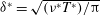 ${\it\delta}^{\ast }=\sqrt{({\it\nu}^{\ast }T^{\ast })/{\rm\pi}}$
are taken as the characteristic temporal and spatial scales of the problem.
${\it\delta}^{\ast }=\sqrt{({\it\nu}^{\ast }T^{\ast })/{\rm\pi}}$
are taken as the characteristic temporal and spatial scales of the problem.
Even though, from a macroscopic point of view, the spheres can be though to rest on the plane wall and to be closely packed, the spheres in the computational box do not touch the plane wall but are
 $0.02D^{\ast }$
away from it,
$0.02D^{\ast }$
away from it,
 $D^{\ast }$
being the sphere diameter. This small gap is required by the numerical implementation of the boundary conditions, which is presently carried out by using the immersed boundary method presented below.
$D^{\ast }$
being the sphere diameter. This small gap is required by the numerical implementation of the boundary conditions, which is presently carried out by using the immersed boundary method presented below.
For similar numerical reasons, a small gap exists between adjacent spheres. The distance (
 ${\it\Delta}_{s}^{\ast }$
) between adjacent spheres is a function of the number of grid points used in each run and is shown in table 1. The reader will notice small variations in the values of
${\it\Delta}_{s}^{\ast }$
) between adjacent spheres is a function of the number of grid points used in each run and is shown in table 1. The reader will notice small variations in the values of
 ${\it\Delta}_{s}$
used in the different runs, which are not expected to affect the results significantly.
${\it\Delta}_{s}$
used in the different runs, which are not expected to affect the results significantly.
Direct numerical simulations of continuity and Navier–Stokes equations are carried out. The dimensionless variables
 $$\begin{eqnarray}\left(x_{1},x_{2},x_{3}\right)=\frac{(x_{1}^{\ast },x_{2}^{\ast },x_{3}^{\ast })}{{\it\delta}^{\ast }},\quad t={\it\omega}^{\ast }t^{\ast },\end{eqnarray}$$
 $$\begin{eqnarray}(u_{1},u_{2},u_{3})=\frac{(u_{1}^{\ast },u_{2}^{\ast },u_{3}^{\ast })}{U_{0}^{\ast }},\quad p=\frac{p^{\ast }}{{\it\rho}^{\ast }(U_{0}^{\ast })^{2}}\end{eqnarray}$$
are introduced, where
 $U_{0}^{\ast }$
and
$U_{0}^{\ast }$
and
 ${\it\omega}^{\ast }(=2{\rm\pi}/T^{\ast })$
are the amplitude and the angular frequency of the velocity oscillations far from the wall respectively. The dimensionless fluid velocity far from the wall turns out to be
${\it\omega}^{\ast }(=2{\rm\pi}/T^{\ast })$
are the amplitude and the angular frequency of the velocity oscillations far from the wall respectively. The dimensionless fluid velocity far from the wall turns out to be
 $$\begin{eqnarray}(u_{1},u_{2},u_{3})_{x_{3}\rightarrow \infty }=(-\!\cos (t),0,0)\end{eqnarray}$$
and is induced by an oscillating pressure gradient out of phase with (2.3) and with amplitude equal to
 ${\it\rho}U_{0}{\it\omega}$
.
${\it\rho}U_{0}{\it\omega}$
.
Table 1. The numerical parameters of the tests.

The boundary conditions force the no-slip condition at the solid boundaries, periodic conditions along the
 $x_{1}$
- and
$x_{1}$
- and
 $x_{2}$
-directions and the free-slip condition at the upper boundary of the computational domain (
$x_{2}$
-directions and the free-slip condition at the upper boundary of the computational domain (
 $x_{3}=L_{x3}$
).
$x_{3}=L_{x3}$
).
Two bottom configurations are considered, characterized by different values of
 $D=D^{\ast }/{\it\delta}^{\ast }$
. The first configuration (configuration A) consists of a layer of spheres, packed in a hexagonal pattern, with a diameter equal to
$D=D^{\ast }/{\it\delta}^{\ast }$
. The first configuration (configuration A) consists of a layer of spheres, packed in a hexagonal pattern, with a diameter equal to
 $6.95{\it\delta}^{\ast }$
(see figure 1). In the second configuration (configuration B), smaller spheres, with a diameter equal to
$6.95{\it\delta}^{\ast }$
(see figure 1). In the second configuration (configuration B), smaller spheres, with a diameter equal to
 $2.32{\it\delta}^{\ast }$
and arranged in a hexagonal pattern, are considered. Values of the Reynolds number
$2.32{\it\delta}^{\ast }$
and arranged in a hexagonal pattern, are considered. Values of the Reynolds number
 $R_{{\it\delta}}=U_{0}^{\ast }{\it\delta}^{\ast }/{\it\nu}^{\ast }$
ranging from moderate values, such that a laminar flow is observed, up to higher values, such that the flow is turbulent, are considered. The parameters of configuration A with
$R_{{\it\delta}}=U_{0}^{\ast }{\it\delta}^{\ast }/{\it\nu}^{\ast }$
ranging from moderate values, such that a laminar flow is observed, up to higher values, such that the flow is turbulent, are considered. The parameters of configuration A with
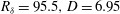
 $R_{{\it\delta}}=95.5$
correspond to those of experiment number 41 by Keiller & Sleath (Reference Keiller and Sleath1976), and the run was used to validate the numerical approach and the postprocessing procedure.
$R_{{\it\delta}}=95.5$
correspond to those of experiment number 41 by Keiller & Sleath (Reference Keiller and Sleath1976), and the run was used to validate the numerical approach and the postprocessing procedure.
A second-order semi-implicit method is used to advance the incompressible Navier–Stokes equations in time. A fractional-step method is employed where convective and diffusive terms are discretized by using third-order Runge–Kutta and Crank–Nicolson schemes respectively. Standard centred second-order finite-difference approximations are used for spatial derivatives.
In order to increase the grid resolution in the region of the computational domain closer to the spheres, the adaptive mesh refinement (AMR) technique (Vanella, Rabenold & Balaras Reference Vanella, Rabenold and Balaras2010) is introduced. The refined grid has an oct-tree structure with a minimum grid size (
 ${\it\Delta}_{min}$
) in the region of the computational domain closer to the spheres and a larger grid size (
${\it\Delta}_{min}$
) in the region of the computational domain closer to the spheres and a larger grid size (
 ${\it\Delta}_{max}$
) in the remaining part of the computational domain. The forcing of the no-slip condition at the surface of the roughness elements is obtained by means of the immersed boundary method by Uhlmann (Reference Uhlmann2005). The immersed boundary method allows a vanishing velocity to be forced on the sphere surface by adding an appropriate forcing term to the discretized Navier–Stokes equations. As a consequence, the governing equations can be numerically integrated on a Cartesian grid without the need to introduce curvilinear coordinates. The AMR technique requires the use of specific multigrid solvers both for the Helmholtz and for the Poisson problems, which arise from the prediction step of the fractional-step scheme and from the continuity equation respectively. The multigrid solvers of both the Helmholtz and Poisson problems are based on the iterative algorithm by Huang & Greengard (Reference Huang and Greengard1999). In particular, the Helmholtz solver uses the alternating direction implicit (ADI) approximate factorization and a ‘local’ direct solver that was specifically developed (M. Mazzuoli and M. Uhlmann, personal communication). The Poisson solver uses a pseudospectral approach and the ‘local’ direct solver developed by Ricker (Reference Ricker2008) and implemented by means of routines of the FLASH code. The dimensions of the computational domain in the streamwise, spanwise and cross-stream (vertical) directions are denoted by
${\it\Delta}_{max}$
) in the remaining part of the computational domain. The forcing of the no-slip condition at the surface of the roughness elements is obtained by means of the immersed boundary method by Uhlmann (Reference Uhlmann2005). The immersed boundary method allows a vanishing velocity to be forced on the sphere surface by adding an appropriate forcing term to the discretized Navier–Stokes equations. As a consequence, the governing equations can be numerically integrated on a Cartesian grid without the need to introduce curvilinear coordinates. The AMR technique requires the use of specific multigrid solvers both for the Helmholtz and for the Poisson problems, which arise from the prediction step of the fractional-step scheme and from the continuity equation respectively. The multigrid solvers of both the Helmholtz and Poisson problems are based on the iterative algorithm by Huang & Greengard (Reference Huang and Greengard1999). In particular, the Helmholtz solver uses the alternating direction implicit (ADI) approximate factorization and a ‘local’ direct solver that was specifically developed (M. Mazzuoli and M. Uhlmann, personal communication). The Poisson solver uses a pseudospectral approach and the ‘local’ direct solver developed by Ricker (Reference Ricker2008) and implemented by means of routines of the FLASH code. The dimensions of the computational domain in the streamwise, spanwise and cross-stream (vertical) directions are denoted by
 $L_{x1}$
 $(L_{x1}=L_{x1}^{\ast }/{\it\delta}^{\ast })$
,
$(L_{x1}=L_{x1}^{\ast }/{\it\delta}^{\ast })$
,
 $L_{x2}$
 $(L_{x2}=L_{x2}^{\ast }/{\it\delta}^{\ast })$
and
$(L_{x2}=L_{x2}^{\ast }/{\it\delta}^{\ast })$
and
 $L_{x3}$
 $(L_{x3}=L_{x3}^{\ast }/{\it\delta}^{\ast })$
respectively. The values of
$(L_{x3}=L_{x3}^{\ast }/{\it\delta}^{\ast })$
respectively. The values of
 $L_{x1}$
,
$L_{x1}$
,
 $L_{x2}$
and
$L_{x2}$
and
 $L_{x3}$
as well as the number of grid points and the number of spheres
$L_{x3}$
as well as the number of grid points and the number of spheres
 $N$
vary from one run to another depending on the values of the dimensionless controlling parameters. The size of the computational box and the number of grid points are chosen by means of a compromise between the accuracy of the results and the computational resources required to obtain them. In order to verify that the size of the computational box was adequate, the two-point correlation of the fluctuating components of the velocity field was considered and it was verified that it tends to vanish as the two-point separation increases (see figure 2).
$N$
vary from one run to another depending on the values of the dimensionless controlling parameters. The size of the computational box and the number of grid points are chosen by means of a compromise between the accuracy of the results and the computational resources required to obtain them. In order to verify that the size of the computational box was adequate, the two-point correlation of the fluctuating components of the velocity field was considered and it was verified that it tends to vanish as the two-point separation increases (see figure 2).

Figure 2. The two-point correlation of the fluctuating velocity components (
 ${\it\chi}=$
streamwise distance,
${\it\chi}=$
streamwise distance,
 ${\it\eta}=$
spanwise distance). (a,c) Configuration A,
${\it\eta}=$
spanwise distance). (a,c) Configuration A,
 $R_{{\it\delta}}=400$
,
$R_{{\it\delta}}=400$
,
 $t=5.06{\rm\pi}$
, distance from the crests of the spheres equal to
$t=5.06{\rm\pi}$
, distance from the crests of the spheres equal to
 $0.0372{\it\delta}$
. (b,d) Configuration B,
$0.0372{\it\delta}$
. (b,d) Configuration B,
 $R_{{\it\delta}}=600$
,
$R_{{\it\delta}}=600$
,
 $t=4.03{\rm\pi}$
, distance from the crests of the spheres equal to
$t=4.03{\rm\pi}$
, distance from the crests of the spheres equal to
 $0.0184{\it\delta}$
. (a,b) Correlation along the streamwise (
$0.0184{\it\delta}$
. (a,b) Correlation along the streamwise (
 $x_{1}$
) direction. (c,d) Correlation along the spanwise (
$x_{1}$
) direction. (c,d) Correlation along the spanwise (
 $x_{2}$
) direction. Solid line
$x_{2}$
) direction. Solid line
 $=$
streamwise velocity, broken line
$=$
streamwise velocity, broken line
 $=$
cross-stream velocity, dash-dot line
$=$
cross-stream velocity, dash-dot line
 $=$
spanwise velocity.
$=$
spanwise velocity.
The adequacy of the number of grid points was verified by considering the 2D spectra of the specific turbulent kinetic energy at different distances from the crests of the spheres. Figure 3, which shows an example of the obtained 2D spectra, allows one to appreciate that the amplitude of the harmonics with large wavenumbers vanishes.

Figure 3. The 2D Fourier transform of the turbulent kinetic energy at a distance from the crests of the spheres equal to
 $0.0372{\it\delta}$
. (a) Configuration A,
$0.0372{\it\delta}$
. (a) Configuration A,
 $R_{{\it\delta}}=400$
,
$R_{{\it\delta}}=400$
,
 $t=6.06{\rm\pi}$
. (b) Configuration B,
$t=6.06{\rm\pi}$
. (b) Configuration B,
 $R_{{\it\delta}}=600$
,
$R_{{\it\delta}}=600$
,
 $t=4{\rm\pi}$
.
$t=4{\rm\pi}$
.
At least two full oscillatory cycles are simulated for all cases and the results of the first cycle are discarded, since they are affected by the initial conditions. It is worthwhile to mention that not all of the obtained flow fields are statistically steady. For this reason the discussion of the results is not based on quantitative values derived from averaged quantities. The values of the parameters of the different runs are given in table 1.
The tests at the highest Reynolds number (
 $R_{{\it\delta}}=600$
) required
$R_{{\it\delta}}=600$
) required
 $\mathit{O}(70\,000)$
time steps per period. The direct numerical simulations of the tests with configuration A were made on two different machines: a 24-core machine (DICCA) and the cluster machine IC2 (KIT Steinbuch Centre for Computing (SCC), Karlsruhe, Germany), requiring approximately 500k CPU hours in total. The tests with configuration B were performed on the BG/Q machine FERMI (CINECA, Bologna, Italy), requiring 1.9 M CPU hours over 1024 cores. The numerical code was designed to efficiently perform on these machines.
$\mathit{O}(70\,000)$
time steps per period. The direct numerical simulations of the tests with configuration A were made on two different machines: a 24-core machine (DICCA) and the cluster machine IC2 (KIT Steinbuch Centre for Computing (SCC), Karlsruhe, Germany), requiring approximately 500k CPU hours in total. The tests with configuration B were performed on the BG/Q machine FERMI (CINECA, Bologna, Italy), requiring 1.9 M CPU hours over 1024 cores. The numerical code was designed to efficiently perform on these machines.
3 The results
3.1 Code validation and processing of the results
To validate the numerical code, a first run was made by fixing the diameter of the spheres and the value of the Reynolds number equal to those of experiment number 41 of Keiller & Sleath (Reference Keiller and Sleath1976). To compare the numerical results with the original measurements of Keiller & Sleath (Reference Keiller and Sleath1976), which were made by using a stationary probe over an oscillating rough bed, in our simulations the numerical probes were oscillated with the outer irrotational velocity. Moreover, since Keiller & Sleath (Reference Keiller and Sleath1976) measured the time development of the modulus of the velocity vector projected on a vertical plane parallel to the direction of the oscillating fluid (indicated with
 $|V|$
), the same quantity was evaluated.
$|V|$
), the same quantity was evaluated.
Figure 4(b) shows the experimental measurements of Keiller & Sleath (Reference Keiller and Sleath1976), while (a) shows the output of the numerical velocity probes, located at distances from the sphere crests equal to the distances used by Keiller & Sleath (Reference Keiller and Sleath1976).

Figure 4. The value of
 $|V|$
at different distances from the crests of the spheres (
$|V|$
at different distances from the crests of the spheres (
 $\,\widetilde{z}\,$
) (
$\,\widetilde{z}\,$
) (
 $R_{{\it\delta}}=95.5$
,
$R_{{\it\delta}}=95.5$
,
 $D=6.95$
). (a) Numerical results with the probes at the same distances as Keiller & Sleath (Reference Keiller and Sleath1976) (–▵–,
$D=6.95$
). (a) Numerical results with the probes at the same distances as Keiller & Sleath (Reference Keiller and Sleath1976) (–▵–,
 $\widetilde{z}=0.2$
; –▫–,
$\widetilde{z}=0.2$
; –▫–,
 $\widetilde{z}=0.42$
; –○–,
$\widetilde{z}=0.42$
; –○–,
 $\widetilde{z}=0.75$
; –▴–,
$\widetilde{z}=0.75$
; –▴–,
 $\widetilde{z}=1.15$
; –●–,
$\widetilde{z}=1.15$
; –●–,
 $\widetilde{z}=2.27$
). (b) Experimental measurements (adapted from Keiller & Sleath (Reference Keiller and Sleath1976)),
$\widetilde{z}=2.27$
). (b) Experimental measurements (adapted from Keiller & Sleath (Reference Keiller and Sleath1976)),
 ${\it\beta}z=x_{3}/{\it\delta}^{\ast }$
.
${\it\beta}z=x_{3}/{\it\delta}^{\ast }$
.
Both the measurements of Keiller & Sleath (Reference Keiller and Sleath1976) and the numerical results show that the velocity close to the bed is characterized by high-frequency oscillations which are related to the passage of the probes over different spheres. Incidentally, let us point out that, for
 $R_{{\it\delta}}=95.5$
, the number of spheres passing the measurement points during a half-stroke is equal to
$R_{{\it\delta}}=95.5$
, the number of spheres passing the measurement points during a half-stroke is equal to
 $U_{0}^{\ast }/({\it\omega}^{\ast }{\it\Delta}_{x1}^{\ast })=3.84$
(
$U_{0}^{\ast }/({\it\omega}^{\ast }{\it\Delta}_{x1}^{\ast })=3.84$
(
 ${\it\Delta}_{x1}^{\ast }=12.43{\it\delta}^{\ast }$
is the distance between the sphere crests along the streamwise direction). The maximum value of
${\it\Delta}_{x1}^{\ast }=12.43{\it\delta}^{\ast }$
is the distance between the sphere crests along the streamwise direction). The maximum value of
 $|V|$
is in phase with the maximum of the outer velocity, which oscillates sinusoidally in time. A further relative maximum can be observed in the form of a sharp peak at a phase close to that of the inversion of the free-stream velocity.
$|V|$
is in phase with the maximum of the outer velocity, which oscillates sinusoidally in time. A further relative maximum can be observed in the form of a sharp peak at a phase close to that of the inversion of the free-stream velocity.
The agreement between experimental and numerical results is fair, even though the comparison shows that the velocity computed by the code is larger than the velocity measured in the experiments. A better agreement with the experimental results of Keiller & Sleath (Reference Keiller and Sleath1976) is obtained if the distance of the numerical probes from the sphere crests is increased. Indeed, if the distance of the numerical probes is increased by
 $0.3{\it\delta}^{\ast }$
, which corresponds to 0.53 mm, a better agreement is observed. Therefore, a small uncertainty in the position of the probes in the experiments of Keiller & Sleath (Reference Keiller and Sleath1976) could partially justify the discrepancy (see figure 4
b).
$0.3{\it\delta}^{\ast }$
, which corresponds to 0.53 mm, a better agreement is observed. Therefore, a small uncertainty in the position of the probes in the experiments of Keiller & Sleath (Reference Keiller and Sleath1976) could partially justify the discrepancy (see figure 4
b).
Moreover, it is worthwhile to remind the reader of the differences between the present arrangement of the spheres and that of Keiller & Sleath (Reference Keiller and Sleath1976). Indeed, in the present simulations the spheres do not touch each other and do not touch the bottom. This small geometrical difference might also partially justify the small differences between the numerical results and the experimental measurements. An estimate of the accuracy of the present results compared with those of Ghodke et al. (Reference Ghodke, Skitka and Apte2014) can be gained by comparing the results plotted in figure 4(a) of Ghodke et al. (Reference Ghodke, Skitka and Apte2014) and the present results plotted in figure 4(a) with the experimental measurements of Keiller & Sleath (Reference Keiller and Sleath1976). Both the measurements of Keiller & Sleath (Reference Keiller and Sleath1976) and the present results show high-frequency oscillations, discussed previously, which are characterized by larger amplitudes during the accelerating phases. The results of Ghodke et al. (Reference Ghodke, Skitka and Apte2014) show high-frequency oscillations of the velocity only during the decelerating phases and are absent during the accelerating phases.
A fair agreement is also found when comparing the present numerical results for the maximum of
 $|V|$
and the phases at which it occurs with the experimental measurements of Keiller & Sleath (Reference Keiller and Sleath1976). Figure 5 shows the present results, the measurements by Keiller & Sleath (Reference Keiller and Sleath1976) and the numerical results of Fornarelli & Vittori (Reference Fornarelli and Vittori2009), who considered a bed covered with half-spheres. Keiller & Sleath (Reference Keiller and Sleath1976) measured, at a distance of
$|V|$
and the phases at which it occurs with the experimental measurements of Keiller & Sleath (Reference Keiller and Sleath1976). Figure 5 shows the present results, the measurements by Keiller & Sleath (Reference Keiller and Sleath1976) and the numerical results of Fornarelli & Vittori (Reference Fornarelli and Vittori2009), who considered a bed covered with half-spheres. Keiller & Sleath (Reference Keiller and Sleath1976) measured, at a distance of
 $0.70{\it\delta}^{\ast }$
from the crests, a maximum of the secondary peak with an amplitude equal to
$0.70{\it\delta}^{\ast }$
from the crests, a maximum of the secondary peak with an amplitude equal to
 $0.49U_{0}^{\ast }$
and a relative phase of
$0.49U_{0}^{\ast }$
and a relative phase of
 $88^{\circ }$
. The present results show a maximum equal to
$88^{\circ }$
. The present results show a maximum equal to
 $0.63U_{0}^{\ast }$
which is attained at a distance from the sphere crests equal to
$0.63U_{0}^{\ast }$
which is attained at a distance from the sphere crests equal to
 $0.68{\it\delta}^{\ast }$
at a relative phase equal to
$0.68{\it\delta}^{\ast }$
at a relative phase equal to
 $40.5^{\circ }$
. As discussed previously, a better agreement with experimental results is attained if the comparison is made after increasing the distance of the numerical probe from the spheres. Indeed, at a distance from the crest equal to
$40.5^{\circ }$
. As discussed previously, a better agreement with experimental results is attained if the comparison is made after increasing the distance of the numerical probe from the spheres. Indeed, at a distance from the crest equal to
 $1.02{\it\delta}^{\ast }$
, the maximum of
$1.02{\it\delta}^{\ast }$
, the maximum of
 $|V|$
is equal to 0.53 and is attained at a phase equal to
$|V|$
is equal to 0.53 and is attained at a phase equal to
 $90^{\circ }$
.
$90^{\circ }$
.

Figure 5. (a) Maxima of
 $|V|$
and (b) their phase (degrees) versus the dimensionless distance from the crests of the roughness elements
$|V|$
and (b) their phase (degrees) versus the dimensionless distance from the crests of the roughness elements
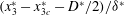 $(x_{3}^{\ast }-x_{3c}^{\ast }-D^{\ast }/2)/{\it\delta}^{\ast }$
. Symbols:
$(x_{3}^{\ast }-x_{3c}^{\ast }-D^{\ast }/2)/{\it\delta}^{\ast }$
. Symbols:
 $^{\ast }$
, computed values;
$^{\ast }$
, computed values;
 $+$
, measured values of Keiller & Sleath (Reference Keiller and Sleath1976);
$+$
, measured values of Keiller & Sleath (Reference Keiller and Sleath1976);
 $\times$
, numerical results of Fornarelli & Vittori (Reference Fornarelli and Vittori2009) (
$\times$
, numerical results of Fornarelli & Vittori (Reference Fornarelli and Vittori2009) (
 $R_{{\it\delta}}=95.5,D=6.95$
).
$R_{{\it\delta}}=95.5,D=6.95$
).
The secondary peaks of
 $|V|$
observed close to flow reversal were assumed to be related to the dynamics of the shear layers, which develop close to the crests of the spheres, by both Keiller & Sleath (Reference Keiller and Sleath1976) and Fornarelli & Vittori (Reference Fornarelli and Vittori2009).
$|V|$
observed close to flow reversal were assumed to be related to the dynamics of the shear layers, which develop close to the crests of the spheres, by both Keiller & Sleath (Reference Keiller and Sleath1976) and Fornarelli & Vittori (Reference Fornarelli and Vittori2009).
Figure 6 shows the time development of the spanwise vorticity component in the mid vertical plane at different phases during the second oscillation cycle. By comparing figure 5 with figure 6 of Fornarelli & Vittori (Reference Fornarelli and Vittori2009) it can be noted that, notwithstanding the differences in the geometry of the roughness elements, the gross dynamics of the vorticity close to the crests is similar. It is worthwhile to point out that the sign of the spanwise vorticity is opposite to that of Fornarelli & Vittori (Reference Fornarelli and Vittori2009) because of the different Cartesian coordinate system used by Fornarelli & Vittori (Reference Fornarelli and Vittori2009).

Figure 6. The non-dimensional spanwise vorticity component (
 ${\it\Omega}_{2}={\it\Omega}_{2}^{\ast }{\it\delta}^{\ast }/U_{0}^{\ast }$
) on the mid plane (
${\it\Omega}_{2}={\it\Omega}_{2}^{\ast }{\it\delta}^{\ast }/U_{0}^{\ast }$
) on the mid plane (
 $x_{2}=14.35$
). The thick solid line indicates vanishing values of
$x_{2}=14.35$
). The thick solid line indicates vanishing values of
 ${\it\Omega}_{2}$
. The dotted curves are isovorticity curves with values of
${\it\Omega}_{2}$
. The dotted curves are isovorticity curves with values of
 ${\it\Omega}_{2}$
equispaced by 0.1. Configuration A (
${\it\Omega}_{2}$
equispaced by 0.1. Configuration A (
 $D=6.95$
),
$D=6.95$
),
 $R_{{\it\delta}}=95.5$
; (a)
$R_{{\it\delta}}=95.5$
; (a)
 $t=4{\rm\pi}$
, (b)
$t=4{\rm\pi}$
, (b)
 $t=4.3{\rm\pi}$
, (c)
$t=4.3{\rm\pi}$
, (c)
 $t=4.4{\rm\pi}$
, (d)
$t=4.4{\rm\pi}$
, (d)
 $t=4.5{\rm\pi}$
.
$t=4.5{\rm\pi}$
.
A key point in the postprocessing of the results is the decomposition of any quantity in the average value and the fluctuating (turbulent) component. In problems where two homogeneous directions can be identified, averaged quantities can be computed by performing a ‘plane average’. In the present case, the average over planes defined by
 $x_{3}=$
constant (taking into account only the regions occupied by the fluid) is denoted by a caret. However, because of the presence of the spheres, the
$x_{3}=$
constant (taking into account only the regions occupied by the fluid) is denoted by a caret. However, because of the presence of the spheres, the
 $x_{1}$
- and
$x_{1}$
- and
 $x_{2}$
-directions are not strictly homogeneous directions and a more appropriate definition of averaged quantities requires the introduction of a conditional average which takes advantage of the particular geometry. In particular, the averaged value of the
$x_{2}$
-directions are not strictly homogeneous directions and a more appropriate definition of averaged quantities requires the introduction of a conditional average which takes advantage of the particular geometry. In particular, the averaged value of the
 $i$
th component of velocity (
$i$
th component of velocity (
 $\overline{u}_{i}$
) is computed as
$\overline{u}_{i}$
) is computed as
 $$\begin{eqnarray}\overline{u}_{i}(X_{1},X_{2},x_{3},t)=\frac{1}{N}\mathop{\sum }_{n=1}^{N}u_{i}^{(n)}(X_{1},X_{2},x_{3},t){\it\phi}(X_{1},X_{2},x_{3}),\end{eqnarray}$$
where
 $X_{1}$
,
$X_{1}$
,
 $X_{2}$
are the streamwise and spanwise coordinates with respect to a system centred on the
$X_{2}$
are the streamwise and spanwise coordinates with respect to a system centred on the
 $n$
th sphere,
$n$
th sphere,
 $N$
is the total number of spheres that are present in the computational domain and
$N$
is the total number of spheres that are present in the computational domain and
 ${\it\phi}$
is a function, defined only outside the spheres, that is equal to 1 at points located inside the hexagonal prism containing the sphere and 0 otherwise. In order to increase the statistical sample, a phase-average procedure was used:
${\it\phi}$
is a function, defined only outside the spheres, that is equal to 1 at points located inside the hexagonal prism containing the sphere and 0 otherwise. In order to increase the statistical sample, a phase-average procedure was used:
 $$\begin{eqnarray}\bar{\bar{f}}(X_{1},X_{2},x_{3},{\it\varphi})=\frac{1}{N_{p}}\mathop{\sum }_{n=0}^{N_{p}-1}\bar{f}(X_{1},X_{2},x_{3},t+2{\rm\pi}n)\quad \text{with }0\leqslant {\it\varphi}<2{\rm\pi},\end{eqnarray}$$
where
 $N_{p}$
indicates the number of available periods.
$N_{p}$
indicates the number of available periods.
Table 2. The values of
 $\langle \widehat{E}_{t}\rangle$
and
$\langle \widehat{E}_{t}\rangle$
and
 $\langle \overline{E}_{t}\rangle$
. The values marked with (*) refer to the second oscillatory cycle (second-last cycle), while the other values are computed considering the last cycle.
$\langle \overline{E}_{t}\rangle$
. The values marked with (*) refer to the second oscillatory cycle (second-last cycle), while the other values are computed considering the last cycle.

Of course, the plane and conditional average procedures provide different values and lead to significant differences in the computed turbulence quantities. These differences are particularly relevant for moderate values of the Reynolds number and configuration A, as can be seen in table 2, which gives the time-average values
 $\langle \overline{E}_{t}\rangle$
,
$\langle \overline{E}_{t}\rangle$
,
 $\langle \widehat{E}_{t}\rangle$
of the bulk turbulent kinetic energy of the flow, defined as
$\langle \widehat{E}_{t}\rangle$
of the bulk turbulent kinetic energy of the flow, defined as
 $$\begin{eqnarray}\langle \overline{E}_{t}\rangle =\frac{1}{2{\rm\pi}}\int _{t}^{t+2{\rm\pi}}\overline{E}_{t}\,\text{d}t,\quad \langle \widehat{E}_{t}\rangle =\frac{1}{2{\rm\pi}}\int _{t}^{t+2{\rm\pi}}\widehat{E}_{t}\,\text{d}t.\end{eqnarray}$$
The quantities
 $\overline{E}_{t}$
and
$\overline{E}_{t}$
and
 $\widehat{E}_{t}$
are computed by volume integration of the specific turbulent kinetic energy, computed using the velocity fluctuations with respect to the conditional-averaged velocity (
$\widehat{E}_{t}$
are computed by volume integration of the specific turbulent kinetic energy, computed using the velocity fluctuations with respect to the conditional-averaged velocity (
 $\overline{e}_{t}$
) and to the plane-averaged velocity (
$\overline{e}_{t}$
) and to the plane-averaged velocity (
 $\widehat{e}_{t}$
) respectively:
$\widehat{e}_{t}$
) respectively:
 $$\begin{eqnarray}\overline{E}_{t}=\frac{1}{S_{h}}\int \overline{e}_{t}\left(X_{1},X_{2},x_{3},t\right)\text{d}X_{1}\,\text{d}X_{2}\,\text{d}x_{3},\quad \widehat{E}_{t}=\int \widehat{e}_{t}(x_{3},t)\,\text{d}x_{3},\end{eqnarray}$$
with
 $$\begin{eqnarray}\displaystyle & \displaystyle \overline{e}_{t}(X_{1},X_{2},x_{3},t)={\textstyle \frac{1}{2}}\left[\overline{(u_{1}-\overline{u}_{1})^{2}}+\overline{(u_{2}-\overline{u}_{2})^{2}}+\overline{(u_{3}-\overline{u}_{3})^{2}}\right], & \displaystyle\end{eqnarray}$$
 $$\begin{eqnarray}\displaystyle & \displaystyle \widehat{e}_{t}(x_{3},t)={\textstyle \frac{1}{2}}\left[\widehat{(u_{1}-\widehat{u}_{1})^{2}}+\widehat{(u_{2}-\widehat{u}_{2})^{2}}+\widehat{(u_{3}-\widehat{u}_{3})^{2}}\right], & \displaystyle\end{eqnarray}$$
 $S_{h}$
is the area of the base of the hexagonal prism that contains the sphere.
$S_{h}$
is the area of the base of the hexagonal prism that contains the sphere.
If the critical conditions for transition to turbulence are determined on the basis of the turbulent kinetic energy, the use of the plane-average procedure might lead to erroneous conclusions, as can be evinced from table 2.
In the following, the fluctuating velocity components
 $u_{i}^{\prime }$
are computed as
$u_{i}^{\prime }$
are computed as
 $$\begin{eqnarray}u_{i}^{\prime }=u_{i}-\overline{u}_{i},\quad i=1,2,3.\end{eqnarray}$$
The high computational costs of the present simulations do not allow simulation of a large number of cycles. Although a phase-average procedure is introduced to increase the statistical sample, in many cases the averaged values are affected by the limited statistical sample. For this reason the largest part of the discussion of the results is not based on statistical quantities, which require an accurate evaluation of the mean quantities. When the discussion of the results involves averaged quantities, only qualitative conclusions are drawn.
3.2 The flow field and vorticity dynamics
The analysis of turbulent kinetic energy allows to identify the different flow regimes which take place as
 $R_{{\it\delta}}$
is increased.
$R_{{\it\delta}}$
is increased.

Figure 7. The time development of the bulk turbulent kinetic energy
 $\overline{E}_{t}$
for all of the runs performed. (a) Configuration A (
$\overline{E}_{t}$
for all of the runs performed. (a) Configuration A (
 $D=6.95$
). (b) Configuration B (
$D=6.95$
). (b) Configuration B (
 $D=2.32$
).
$D=2.32$
).
In configuration A (
 $D=6.95$
),
$D=6.95$
),
 $\overline{E}_{t}$
is negligible throughout the cycle for
$\overline{E}_{t}$
is negligible throughout the cycle for
 $R_{{\it\delta}}=95.5$
and the flow regime can be defined as laminar (see figure 7
a). For higher values of
$R_{{\it\delta}}=95.5$
and the flow regime can be defined as laminar (see figure 7
a). For higher values of
 $R_{{\it\delta}}$
,
$R_{{\it\delta}}$
,
 $\overline{E}_{t}$
increases during the accelerating phases and reaches its maximum value in the early decelerating phases (see figure 7
a). The increase of the turbulent kinetic energy in configuration A is due to the presence of large vortex structures, the dynamics of which differ from sphere to sphere. As time progresses, due to nonlinear effects, smaller vortex structures are formed, which induce large values of the turbulent kinetic energy. The turbulent kinetic energy during the late accelerating phases has the same order of magnitude as that characterizing the decelerating phases.
$\overline{E}_{t}$
increases during the accelerating phases and reaches its maximum value in the early decelerating phases (see figure 7
a). The increase of the turbulent kinetic energy in configuration A is due to the presence of large vortex structures, the dynamics of which differ from sphere to sphere. As time progresses, due to nonlinear effects, smaller vortex structures are formed, which induce large values of the turbulent kinetic energy. The turbulent kinetic energy during the late accelerating phases has the same order of magnitude as that characterizing the decelerating phases.
Figure 7(b) shows that, in configuration B (
 $D=2.32$
),
$D=2.32$
),
 $\overline{E}_{t}$
increases during the decelerating part of the cycle. Even though flow separation certainly plays a role in the transition process in configuration B, the transition process is more similar to that observed in the flat wall case by Vittori & Verzicco (Reference Vittori and Verzicco1998).
$\overline{E}_{t}$
increases during the decelerating part of the cycle. Even though flow separation certainly plays a role in the transition process in configuration B, the transition process is more similar to that observed in the flat wall case by Vittori & Verzicco (Reference Vittori and Verzicco1998).
Figure 8 shows the values of
 $\langle \overline{E}_{t}\rangle$
as a function both of the Reynolds numbers
$\langle \overline{E}_{t}\rangle$
as a function both of the Reynolds numbers
 $R_{{\it\delta}}$
and
$R_{{\it\delta}}$
and
 $Re=(U_{0}^{\ast }D^{\ast })/{\it\nu}$
. In configuration A, the increase of
$Re=(U_{0}^{\ast }D^{\ast })/{\it\nu}$
. In configuration A, the increase of
 $\langle \overline{E}_{t}\rangle$
with
$\langle \overline{E}_{t}\rangle$
with
 $R_{{\it\delta}}$
, which indicates departure from the laminar regime, takes place for
$R_{{\it\delta}}$
, which indicates departure from the laminar regime, takes place for
 $R_{{\it\delta}}$
ranging from 95.5 to 150 or, equivalently, for
$R_{{\it\delta}}$
ranging from 95.5 to 150 or, equivalently, for
 $Re$
ranging from 664 to 1042. The results for the configuration with smaller spheres (configuration B) show non-vanishing values of
$Re$
ranging from 664 to 1042. The results for the configuration with smaller spheres (configuration B) show non-vanishing values of
 $\overline{E}_{t}$
only for the highest value of
$\overline{E}_{t}$
only for the highest value of
 $R_{{\it\delta}}$
(
$R_{{\it\delta}}$
(
 $R_{{\it\delta}}=600$
,
$R_{{\it\delta}}=600$
,
 $Re=1392$
) and during the last oscillatory cycle of the run with
$Re=1392$
) and during the last oscillatory cycle of the run with
 $R_{{\it\delta}}=500$
(
$R_{{\it\delta}}=500$
(
 $Re=1160$
). As discussed in the following, the flow field for
$Re=1160$
). As discussed in the following, the flow field for
 $R_{{\it\delta}}$
equal to 500 shows transitional characteristics, which make the values of both
$R_{{\it\delta}}$
equal to 500 shows transitional characteristics, which make the values of both
 $\overline{E}_{t}$
and
$\overline{E}_{t}$
and
 $\langle \overline{E}_{t}\rangle$
significantly different when computed during the last and second-last oscillatory cycles (see table 2 and figure 8).
$\langle \overline{E}_{t}\rangle$
significantly different when computed during the last and second-last oscillatory cycles (see table 2 and figure 8).

Figure 8. The time-averaged bulk turbulent kinetic energy (
 $\langle \overline{E}_{t}\rangle$
) versus
$\langle \overline{E}_{t}\rangle$
) versus
 $R_{{\it\delta}}$
for all the runs performed (a) and versus
$R_{{\it\delta}}$
for all the runs performed (a) and versus
 $Re=(U_{0}^{\ast }D^{\ast })/{\it\nu}^{\ast }$
(b):
$Re=(U_{0}^{\ast }D^{\ast })/{\it\nu}^{\ast }$
(b):
 $\circ =$
configuration A (
$\circ =$
configuration A (
 $D=6.95$
);
$D=6.95$
);
 $\ast =$
configuration B (
$\ast =$
configuration B (
 $D=2.32$
) with the average computed over the second cycle; ▫
$D=2.32$
) with the average computed over the second cycle; ▫
 $=$
configuration B (
$=$
configuration B (
 $D=2.32$
) with the average computed over the third cycle.
$D=2.32$
) with the average computed over the third cycle.
Table 3. The maximum values of the dimensionless vorticity components computed over the last oscillatory cycle. The values marked with (*) refer to the second oscillatory cycle.

Figures 7, 8 and the evolution of vorticity discussed in the following allow different flow regimes to be identified. The laminar regime is observed in configuration A only for
 $R_{{\it\delta}}=95.5$
, while in configuration B it is observed up to
$R_{{\it\delta}}=95.5$
, while in configuration B it is observed up to
 $R_{{\it\delta}}=500$
. Two turbulent regimes are identified, which are named the ‘transitional turbulent regime’ and the ‘hydrodynamically rough turbulent regime’. The former is observed in configuration B for
$R_{{\it\delta}}=500$
. Two turbulent regimes are identified, which are named the ‘transitional turbulent regime’ and the ‘hydrodynamically rough turbulent regime’. The former is observed in configuration B for
 $R_{{\it\delta}}=600$
and during the third oscillatory cycle for
$R_{{\it\delta}}=600$
and during the third oscillatory cycle for
 $R_{{\it\delta}}=500$
. The transitional turbulent regime is characterized by large values of the turbulent kinetic energy which are mainly confined to the decelerating phases and are related to the formation of small turbulent eddies. These turbulent eddies are generated by the intrinsic instability of the oscillatory Stokes flow with a small contribution from the bottom roughness. The hydrodynamically rough turbulent regime, which is characterized by fluctuations that appear to be more influenced by the presence of the roughness than by a mere instability process, is observed only in configuration A and for values of the Reynolds number larger than 100.
$R_{{\it\delta}}=500$
. The transitional turbulent regime is characterized by large values of the turbulent kinetic energy which are mainly confined to the decelerating phases and are related to the formation of small turbulent eddies. These turbulent eddies are generated by the intrinsic instability of the oscillatory Stokes flow with a small contribution from the bottom roughness. The hydrodynamically rough turbulent regime, which is characterized by fluctuations that appear to be more influenced by the presence of the roughness than by a mere instability process, is observed only in configuration A and for values of the Reynolds number larger than 100.
In the following, the conclusions derived on the basis of the analysis of the turbulent kinetic energy will be confirmed by the analysis of the vorticity fields and of the forces exerted on the spheres.
In all of the runs, the maximum of the spanwise component of the vorticity (
 ${\it\Omega}_{2}$
) is larger than the maxima of the streamwise and cross-stream components (see table 3). The maximum of the cross-stream component of vorticity (
${\it\Omega}_{2}$
) is larger than the maxima of the streamwise and cross-stream components (see table 3). The maximum of the cross-stream component of vorticity (
 ${\it\Omega}_{3}$
) is larger than the maximum of the streamwise component and, as the Reynolds number is increased, the three components of the vorticity tend to assume comparable values. For the same value of
${\it\Omega}_{3}$
) is larger than the maximum of the streamwise component and, as the Reynolds number is increased, the three components of the vorticity tend to assume comparable values. For the same value of
 $R_{{\it\delta}}$
, the maximum values attained by
$R_{{\it\delta}}$
, the maximum values attained by
 ${\it\Omega}_{1}$
and
${\it\Omega}_{1}$
and
 ${\it\Omega}_{3}$
for configuration A are larger than the corresponding values for configuration B. This indicates that the runs for configuration B are characterized by smaller convective effects than configuration A.
${\it\Omega}_{3}$
for configuration A are larger than the corresponding values for configuration B. This indicates that the runs for configuration B are characterized by smaller convective effects than configuration A.
The time development of the spanwise component of the vorticity
 ${\it\Omega}_{2}$
, plotted in figures 9 and 10, shows that
${\it\Omega}_{2}$
, plotted in figures 9 and 10, shows that
 ${\it\Omega}_{2}$
is generated at the sphere crests during the accelerating phases of the cycle and is associated with the formation of shear layers. In configuration A and for the lower values of
${\it\Omega}_{2}$
is generated at the sphere crests during the accelerating phases of the cycle and is associated with the formation of shear layers. In configuration A and for the lower values of
 $R_{{\it\delta}}$
(see figure 9), when the flow falls in the laminar regime, long streaks of vorticity, characterized by values of
$R_{{\it\delta}}$
(see figure 9), when the flow falls in the laminar regime, long streaks of vorticity, characterized by values of
 ${\it\Omega}_{2}$
of the same sign, form immediately above the sphere crests when the flow accelerates. These streaks eventually lift from the bottom, dissipate and reform with vorticity of opposite sign during the following half-cycle. For larger values of
${\it\Omega}_{2}$
of the same sign, form immediately above the sphere crests when the flow accelerates. These streaks eventually lift from the bottom, dissipate and reform with vorticity of opposite sign during the following half-cycle. For larger values of
 $R_{{\it\delta}}$
, so that the flow falls in the hydrodynamically rough turbulent regime, regular long streaks of spanwise vorticity cannot be recognized. Indeed, shortly after the formation of the spanwise vorticity at the crests, the regions with high values of
$R_{{\it\delta}}$
, so that the flow falls in the hydrodynamically rough turbulent regime, regular long streaks of spanwise vorticity cannot be recognized. Indeed, shortly after the formation of the spanwise vorticity at the crests, the regions with high values of
 ${\it\Omega}_{2}$
elongate in the flow direction, interact with the crest of the following spheres, break and lift from the bottom. Small regions of vorticity of opposite sign are observed at the end of the accelerating phase, when the vorticity shed from the crests breaks up into small vortex structures.
${\it\Omega}_{2}$
elongate in the flow direction, interact with the crest of the following spheres, break and lift from the bottom. Small regions of vorticity of opposite sign are observed at the end of the accelerating phase, when the vorticity shed from the crests breaks up into small vortex structures.

Figure 9. Isocontours of the dimensionless spanwise component of vorticity (
 ${\it\Omega}_{2}={\it\Omega}_{2}^{\ast }{\it\delta}^{\ast }/U_{0}^{\ast }$
),
${\it\Omega}_{2}={\it\Omega}_{2}^{\ast }{\it\delta}^{\ast }/U_{0}^{\ast }$
),
 ${\it\Omega}_{2}=\pm 0.446$
. Light grey (green online)
${\it\Omega}_{2}=\pm 0.446$
. Light grey (green online)
 $=$
positive vorticity, dark grey (red online)
$=$
positive vorticity, dark grey (red online)
 $=$
negative vorticity;
$=$
negative vorticity;
 $R_{{\it\delta}}=95.5$
. Configuration A (
$R_{{\it\delta}}=95.5$
. Configuration A (
 $D=6.95$
): (a)
$D=6.95$
): (a)
 $t=0.75{\rm\pi}$
, (b)
$t=0.75{\rm\pi}$
, (b)
 $t={\rm\pi}$
, (c)
$t={\rm\pi}$
, (c)
 $t=1.25{\rm\pi}$
, (d)
$t=1.25{\rm\pi}$
, (d)
 $t=1.5{\rm\pi}$
.
$t=1.5{\rm\pi}$
.

Figure 10. Isocontours of the dimensionless spanwise component of vorticity (
 ${\it\Omega}_{2}={\it\Omega}_{2}^{\ast }{\it\delta}^{\ast }/U_{0}^{\ast }$
),
${\it\Omega}_{2}={\it\Omega}_{2}^{\ast }{\it\delta}^{\ast }/U_{0}^{\ast }$
),
 ${\it\Omega}_{2}=\pm 0.70$
. Light grey (green online)
${\it\Omega}_{2}=\pm 0.70$
. Light grey (green online)
 $=$
positive vorticity, dark grey (red online)
$=$
positive vorticity, dark grey (red online)
 $=$
negative vorticity;
$=$
negative vorticity;
 $R_{{\it\delta}}=600$
. Configuration B (
$R_{{\it\delta}}=600$
. Configuration B (
 $D=2.32$
): (a)
$D=2.32$
): (a)
 $t=0.75{\rm\pi}$
, (b)
$t=0.75{\rm\pi}$
, (b)
 $t={\rm\pi}$
, (c)
$t={\rm\pi}$
, (c)
 $t=1.13{\rm\pi}$
, (d)
$t=1.13{\rm\pi}$
, (d)
 $t=1.22{\rm\pi}$
.
$t=1.22{\rm\pi}$
.
In configuration B, the vorticity field shows a clear spatial and temporal periodicity up to
 $R_{{\it\delta}}=500$
. For
$R_{{\it\delta}}=500$
. For
 $R_{{\it\delta}}=600$
, towards the late accelerating and early decelerating phases, the spanwise vorticity, released from the top of the spheres, forms streaks elongated in the streamwise direction (see figure 10) which then break into small eddies and turbulence appears.
$R_{{\it\delta}}=600$
, towards the late accelerating and early decelerating phases, the spanwise vorticity, released from the top of the spheres, forms streaks elongated in the streamwise direction (see figure 10) which then break into small eddies and turbulence appears.
The cross-stream component of vorticity
 ${\it\Omega}_{3}$
is first generated at the sides of the spheres and, as time progresses, is convected downstream. In configuration A, the convection of
${\it\Omega}_{3}$
is first generated at the sides of the spheres and, as time progresses, is convected downstream. In configuration A, the convection of
 ${\it\Omega}_{3}$
causes the formation of streaks of cross-stream vorticity of alternating sign (see figure 11). The presence of bands of cross-stream vorticity of alternate sign suggests the formation of low- and high-speed streaks in the region immediately above the crests. The streaks dissipate during the decelerating phase and a specular flow field is generated when the free-stream flow reverses. As the Reynolds number is increased, the streaks of cross-stream vorticity (
${\it\Omega}_{3}$
causes the formation of streaks of cross-stream vorticity of alternating sign (see figure 11). The presence of bands of cross-stream vorticity of alternate sign suggests the formation of low- and high-speed streaks in the region immediately above the crests. The streaks dissipate during the decelerating phase and a specular flow field is generated when the free-stream flow reverses. As the Reynolds number is increased, the streaks of cross-stream vorticity (
 ${\it\Omega}_{3}$
) become more irregular, lift from the crests of the spheres, due to their interaction with the following spheres, break up and dissipate more quickly than the cases at lower values of
${\it\Omega}_{3}$
) become more irregular, lift from the crests of the spheres, due to their interaction with the following spheres, break up and dissipate more quickly than the cases at lower values of
 $R_{{\it\delta}}$
. In configuration B, the convection of cross-stream vorticity by the mean flow is weaker and no streaks are observed for values of the Reynolds number up to 500. For
$R_{{\it\delta}}$
. In configuration B, the convection of cross-stream vorticity by the mean flow is weaker and no streaks are observed for values of the Reynolds number up to 500. For
 $R_{{\it\delta}}=600$
(see figure 12), when the flow falls in the transitional regime, streaks are observed during the late acceleration and early decelerating phases. Then, as the flow decelerates, the streaks break up and vorticity is ejected far from the wall. A similar evolution was observed by Costamagna et al. (Reference Costamagna, Vittori and Blondeaux2003), who reported the formation of ejection events in the oscillatory boundary layer over a smooth wall.
$R_{{\it\delta}}=600$
(see figure 12), when the flow falls in the transitional regime, streaks are observed during the late acceleration and early decelerating phases. Then, as the flow decelerates, the streaks break up and vorticity is ejected far from the wall. A similar evolution was observed by Costamagna et al. (Reference Costamagna, Vittori and Blondeaux2003), who reported the formation of ejection events in the oscillatory boundary layer over a smooth wall.

Figure 11. Isocontours of the dimensionless cross-stream component of vorticity (
 ${\it\Omega}_{3}={\it\Omega}_{3}^{\ast }{\it\delta}^{\ast }/U_{0}^{\ast }$
),
${\it\Omega}_{3}={\it\Omega}_{3}^{\ast }{\it\delta}^{\ast }/U_{0}^{\ast }$
),
 ${\it\Omega}_{3}=\pm 0.20$
. Light grey (green online)
${\it\Omega}_{3}=\pm 0.20$
. Light grey (green online)
 $=$
positive vorticity, dark grey (red online)
$=$
positive vorticity, dark grey (red online)
 $=$
negative vorticity;
$=$
negative vorticity;
 $R_{{\it\delta}}=95.5$
. Configuration A (
$R_{{\it\delta}}=95.5$
. Configuration A (
 $D=6.95$
): (a)
$D=6.95$
): (a)
 $t=0.63{\rm\pi}$
, (b)
$t=0.63{\rm\pi}$
, (b)
 $t={\rm\pi}$
, (c)
$t={\rm\pi}$
, (c)
 $t=1.25{\rm\pi}$
, (d)
$t=1.25{\rm\pi}$
, (d)
 $t=1.55{\rm\pi}$
.
$t=1.55{\rm\pi}$
.

Figure 12. Isocontours of the dimensionless cross-stream component of vorticity (
 ${\it\Omega}_{3}={\it\Omega}_{3}^{\ast }{\it\delta}^{\ast }/U_{0}^{\ast }$
),
${\it\Omega}_{3}={\it\Omega}_{3}^{\ast }{\it\delta}^{\ast }/U_{0}^{\ast }$
),
 ${\it\Omega}_{3}=\pm 0.515$
. Light grey (green online)
${\it\Omega}_{3}=\pm 0.515$
. Light grey (green online)
 $=$
positive vorticity, dark grey (red online)
$=$
positive vorticity, dark grey (red online)
 $=$
negative vorticity;
$=$
negative vorticity;
 $R_{{\it\delta}}=600$
. Configuration B (
$R_{{\it\delta}}=600$
. Configuration B (
 $D=2.32$
): (a)
$D=2.32$
): (a)
 $t=0.63{\rm\pi}$
, (b)
$t=0.63{\rm\pi}$
, (b)
 $t={\rm\pi}$
, (c)
$t={\rm\pi}$
, (c)
 $t=1.19{\rm\pi}$
, (d)
$t=1.19{\rm\pi}$
, (d)
 $t=1.29{\rm\pi}$
.
$t=1.29{\rm\pi}$
.
The streamwise component of the vorticity
 ${\it\Omega}_{1}$
, for both configurations A and B, is similar to that of
${\it\Omega}_{1}$
, for both configurations A and B, is similar to that of
 ${\it\Omega}_{3}$
. In configuration A,
${\it\Omega}_{3}$
. In configuration A,
 ${\it\Omega}_{1}$
is generated during the decelerating phases at the sides of the spheres and builds up during the accelerating phases. The regions of high values of
${\it\Omega}_{1}$
is generated during the decelerating phases at the sides of the spheres and builds up during the accelerating phases. The regions of high values of
 ${\it\Omega}_{1}$
are convected by the mean flow and the value of
${\it\Omega}_{1}$
are convected by the mean flow and the value of
 ${\it\Omega}_{1}$
increases due to the stretching of vorticity by the flow. During the decelerating phases the vortex structures are rapidly dissipated.
${\it\Omega}_{1}$
increases due to the stretching of vorticity by the flow. During the decelerating phases the vortex structures are rapidly dissipated.
In configuration B and for
 $R_{{\it\delta}}=600$
, the regions with high values of
$R_{{\it\delta}}=600$
, the regions with high values of
 ${\it\Omega}_{1}$
organize into streaks which eventually break up and are ejected far from the wall.
${\it\Omega}_{1}$
organize into streaks which eventually break up and are ejected far from the wall.
In configuration B and for
 $R_{{\it\delta}}=500$
, the flow shows peculiar characteristics. Indeed, the evolution of vorticity during the second oscillatory cycle is similar to that observed for lower values of
$R_{{\it\delta}}=500$
, the flow shows peculiar characteristics. Indeed, the evolution of vorticity during the second oscillatory cycle is similar to that observed for lower values of
 $R_{{\it\delta}}$
. Then, during the second decelerating phase of the third oscillatory cycle, large disturbances, similar to Tollmien–Schlichting waves, appear. The vorticity released from the crests of the spheres is subject to oscillations with a clear streamwise and temporal periodicity (see figure 13 and supplementary movie 1 available at http://dx.doi.org/10.1017/jfm.2016.61). As time progresses, the amplitude of the oscillations increases and eventually the large coherent vortex structures break, generating small eddies which later dissipate. The whole process takes place over a limited time interval during the decelerating phase, precisely for
$R_{{\it\delta}}$
. Then, during the second decelerating phase of the third oscillatory cycle, large disturbances, similar to Tollmien–Schlichting waves, appear. The vorticity released from the crests of the spheres is subject to oscillations with a clear streamwise and temporal periodicity (see figure 13 and supplementary movie 1 available at http://dx.doi.org/10.1017/jfm.2016.61). As time progresses, the amplitude of the oscillations increases and eventually the large coherent vortex structures break, generating small eddies which later dissipate. The whole process takes place over a limited time interval during the decelerating phase, precisely for
 $t$
ranging from
$t$
ranging from
 $5{\rm\pi}$
to
$5{\rm\pi}$
to
 $5.33{\rm\pi}$
. The quantity
$5.33{\rm\pi}$
. The quantity
 ${\it\lambda}_{2}$
, introduced by Jeong & Hussain (Reference Jeong and Hussain1995) to detect coherent vortex structures, shows that when the large disturbances appear for
${\it\lambda}_{2}$
, introduced by Jeong & Hussain (Reference Jeong and Hussain1995) to detect coherent vortex structures, shows that when the large disturbances appear for
 $R_{{\it\delta}}=500$
, horseshoe vortices form upstream of the spheres while the structures released from the crests generate hairpin vortices (see figure 14 and supplementary movie 1). A similar pattern of coherent structures was observed around isolated hemispherical roughness elements in steady boundary layers by Acarlar & Smith (Reference Acarlar and Smith1987) and Zhou, Wang & Fan (Reference Zhou, Wang and Fan2010).
$R_{{\it\delta}}=500$
, horseshoe vortices form upstream of the spheres while the structures released from the crests generate hairpin vortices (see figure 14 and supplementary movie 1). A similar pattern of coherent structures was observed around isolated hemispherical roughness elements in steady boundary layers by Acarlar & Smith (Reference Acarlar and Smith1987) and Zhou, Wang & Fan (Reference Zhou, Wang and Fan2010).

Figure 13. Isocontours of the dimensionless (a) streamwise (
 $|{\it\Omega}_{1}|=\pm 0.116$
) and (b) cross-stream (
$|{\it\Omega}_{1}|=\pm 0.116$
) and (b) cross-stream (
 $|{\it\Omega}_{3}|=\pm 0.177$
) components of vorticity at
$|{\it\Omega}_{3}|=\pm 0.177$
) components of vorticity at
 $t=5.19{\rm\pi}$
;
$t=5.19{\rm\pi}$
;
 $R_{{\it\delta}}=500$
, configuration B (
$R_{{\it\delta}}=500$
, configuration B (
 $D=2.32$
): light grey (green online)
$D=2.32$
): light grey (green online)
 $=$
positive vorticity, dark grey (red online)
$=$
positive vorticity, dark grey (red online)
 $=$
negative vorticity.
$=$
negative vorticity.

Figure 14. Isosurfaces of
 ${\it\lambda}_{2}$
(
${\it\lambda}_{2}$
(
 ${\it\lambda}_{2}=-0.11$
);
${\it\lambda}_{2}=-0.11$
);
 $R_{{\it\delta}}=500$
,
$R_{{\it\delta}}=500$
,
 $t=5.08{\rm\pi}$
, configuration B (
$t=5.08{\rm\pi}$
, configuration B (
 $D=2.32$
).
$D=2.32$
).
3.3 Hydrodynamic force on the spheres
Knowledge of the velocity and pressure fields allows evaluation of the strain rate tensor, the viscous stresses and the force acting on the roughness elements. In the two turbulent regimes previously identified, the force shows a dependence on the sphere considered, due to the random variations of the vortex structures and the subsequent formation of smaller vortices characterized by a random spatial distribution. In order to provide information on the general characteristics of the force exerted on the roughness elements, the force averaged over all of the spheres (
 $\overline{F}_{x1},\overline{F}_{x2},\overline{F}_{x3}$
) is presented. The force averaged over all spheres is decomposed into a contribution related to pressure
$\overline{F}_{x1},\overline{F}_{x2},\overline{F}_{x3}$
) is presented. The force averaged over all spheres is decomposed into a contribution related to pressure
 $(\overline{F}_{x1}^{(p)},\overline{F}_{x2}^{(p)},\overline{F}_{x3}^{(p)})$
and a contribution related to viscous stresses
$(\overline{F}_{x1}^{(p)},\overline{F}_{x2}^{(p)},\overline{F}_{x3}^{(p)})$
and a contribution related to viscous stresses
 $(\overline{F}_{x1}^{(v)},\overline{F}_{x2}^{(v)},\overline{F}_{x3}^{(v)})$
:
$(\overline{F}_{x1}^{(v)},\overline{F}_{x2}^{(v)},\overline{F}_{x3}^{(v)})$
:
 $$\begin{eqnarray}(\overline{F}_{x1}^{(p)},\overline{F}_{x2}^{(p)},\overline{F}_{x3}^{(p)})=\int _{S}(-\overline{p}n_{x1},-\overline{p}n_{x2},-\overline{p}~n_{x3})\,\text{d}S,\end{eqnarray}$$
 $$\begin{eqnarray}(\overline{F}_{x1}^{(v)},\overline{F}_{x2}^{(v)},\overline{F}_{x3}^{(v)})=\int _{S}\left[(\overline{t}_{x1},\overline{t}_{x2},\overline{t}_{x3})+(\overline{p}~n_{x1},\overline{p}~n_{x2},\overline{p}~n_{x3})\right]\text{d}S,\end{eqnarray}$$
where
 $(n_{x1},n_{x2},n_{x3})$
is the unit vector orthogonal to the surface
$(n_{x1},n_{x2},n_{x3})$
is the unit vector orthogonal to the surface
 $S$
of the sphere and
$S$
of the sphere and
 $(\overline{t}_{x1},\overline{t}_{x2},\overline{t}_{x3})$
is the average (dimensionless) stress exerted by the fluid on
$(\overline{t}_{x1},\overline{t}_{x2},\overline{t}_{x3})$
is the average (dimensionless) stress exerted by the fluid on
 $S$
, which is scaled as the pressure. The force components are made dimensionless using the quantity
$S$
, which is scaled as the pressure. The force components are made dimensionless using the quantity
 ${\it\rho}^{\ast }U_{0}^{\ast 2}{\it\delta}^{\ast 2}$
.
${\it\rho}^{\ast }U_{0}^{\ast 2}{\it\delta}^{\ast 2}$
.
Figure 15 shows the streamwise and cross-stream force components, along with the corresponding components computed by Fornarelli & Vittori (Reference Fornarelli and Vittori2009). In the same figure, the viscous and pressure contributions are also shown in (b) and (c) respectively. The streamwise component of the force of the present study has a time development similar to that computed by Fornarelli & Vittori (Reference Fornarelli and Vittori2009), even though its maximum value lags ahead of that evaluated by Fornarelli & Vittori (Reference Fornarelli and Vittori2009). Indeed, both the viscous and pressure contributions show a maximum that takes place before that evaluated by Fornarelli & Vittori (Reference Fornarelli and Vittori2009). As discussed later, this difference is due to the force exerted by the fluid on the lower half of the surface of the spheres, which is not present in the computations of Fornarelli & Vittori (Reference Fornarelli and Vittori2009).

Figure 15. The time development of the averaged streamwise and cross-stream components of the force (a) exerted on the spherical roughness element, of its viscous component (b) and of its pressure component (c). Thick lines
 $=$
streamwise component, thin lines
$=$
streamwise component, thin lines
 $=$
cross-stream component; present geometry
$=$
cross-stream component; present geometry
 $=$
solid lines, Fornarelli & Vittori (Reference Fornarelli and Vittori2009)
$=$
solid lines, Fornarelli & Vittori (Reference Fornarelli and Vittori2009)
 $=$
broken lines. All quantities are made non-dimensional by means of
$=$
broken lines. All quantities are made non-dimensional by means of
 ${\it\rho}U_{0}^{\ast 2}{\it\delta}^{\ast 2}$
.
${\it\rho}U_{0}^{\ast 2}{\it\delta}^{\ast 2}$
.
The cross-stream component of the force is characterized by a time development grossly similar to that observed by Fornarelli & Vittori (Reference Fornarelli and Vittori2009). However, the present results show clearly the presence of a secondary peak close to flow reversal, which is related to the formation of areas of positive pressure on the lower downstream surface of the spheres, as discussed in the following. Moreover, differently from Fornarelli & Vittori (Reference Fornarelli and Vittori2009), during the decelerating phases of the cycle, the present results show negative values of the cross-stream component of the force. A lift force directed towards the wall has also been observed by Rosenthal & Sleath (Reference Rosenthal and Sleath1986), who measured the lift force on an isolated sphere close to a wall in an oscillatory boundary layer. This effect appears to be related to the anticipated flow reversal near the wall, which causes the formation of areas of negative pressure on the lower surface of the spheres.
The viscous contribution to the cross-stream force is much smaller than the pressure contribution both for present results and for those of Fornarelli & Vittori (Reference Fornarelli and Vittori2009).
The comparison of the present results with those of Fornarelli & Vittori (Reference Fornarelli and Vittori2009), who considered half-spheres as roughness elements, shows that the details of the geometry of the roughness elements have a small influence on the velocity field above the roughness elements (see the previous section), but have a significant effect on the force, because the lower part of the sphere surface contributes significantly to the total force.
The time development of the averaged force components is plotted in figures 16 and 17 for all of the Reynolds numbers presently simulated and for configurations A and B respectively. The spanwise component of the force, as expected, turns out to be negligible and it is not shown in figures 16 and 17.

Figure 16. The time development of the streamwise (a) and cross-stream (b) components of the dimensionless force (
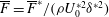 $\overline{F}=\overline{F}^{\ast }/({\it\rho}U_{0}^{\ast 2}{\it\delta}^{\ast 2})$
), averaged over all of the spheres, for all of the considered values of
$\overline{F}=\overline{F}^{\ast }/({\it\rho}U_{0}^{\ast 2}{\it\delta}^{\ast 2})$
), averaged over all of the spheres, for all of the considered values of
 $R_{{\it\delta}}$
and for configuration A (
$R_{{\it\delta}}$
and for configuration A (
 $D=6.95$
). The thick-dotted line (blue online) indicates the time development of the velocity outside the boundary layer.
$D=6.95$
). The thick-dotted line (blue online) indicates the time development of the velocity outside the boundary layer.

Figure 17. The time development of the streamwise (a) and cross-stream (b) components of the dimensionless force (
 $\overline{F}=\overline{F}^{\ast }/({\it\rho}U_{0}^{\ast 2}{\it\delta}^{\ast 2})$
), averaged over all of the spheres, for all of the considered values of
$\overline{F}=\overline{F}^{\ast }/({\it\rho}U_{0}^{\ast 2}{\it\delta}^{\ast 2})$
), averaged over all of the spheres, for all of the considered values of
 $R_{{\it\delta}}$
and for configuration B (
$R_{{\it\delta}}$
and for configuration B (
 $D=2.32$
). The thick-dotted line (blue online) indicates the time development of the velocity outside the boundary layer.
$D=2.32$
). The thick-dotted line (blue online) indicates the time development of the velocity outside the boundary layer.
Often, for practical purposes, the streamwise component of the force is decomposed into a part proportional to the external velocity and a part proportional to the external acceleration. The present results show that the latter contribution prevails over the former.
Table 4 shows the module of the drag exerted by the fluid on the spheres (
 $\bar{\bar{F_{x}}}^{(s)}$
) and on the plane wall (
$\bar{\bar{F_{x}}}^{(s)}$
) and on the plane wall (
 $\bar{\bar{F_{x}}}^{(w)}$
), averaged over the half-oscillation-period during which the free-stream velocity is either positive or negative.
$\bar{\bar{F_{x}}}^{(w)}$
), averaged over the half-oscillation-period during which the free-stream velocity is either positive or negative.
Table 4. The drag force on the spheres (
 $\bar{\bar{F_{x}}}^{(s)}$
) and on the plane wall (
$\bar{\bar{F_{x}}}^{(s)}$
) and on the plane wall (
 $\bar{\bar{F_{x}}}^{(w)}$
), averaged over the half-oscillation-period.
$\bar{\bar{F_{x}}}^{(w)}$
), averaged over the half-oscillation-period.

The cross-stream component of the force (
 $\overline{F}_{x3}$
) is mainly related to the effect of pressure and attains its maximum value later than
$\overline{F}_{x3}$
) is mainly related to the effect of pressure and attains its maximum value later than
 $\overline{F}_{x1}$
. In configuration A and for
$\overline{F}_{x1}$
. In configuration A and for
 $R_{{\it\delta}}=95.5$
,
$R_{{\it\delta}}=95.5$
,
 $\overline{F}_{x3}$
shows a secondary peak close to flow reversal (see figure 16), which has been discussed previously. For higher values of
$\overline{F}_{x3}$
shows a secondary peak close to flow reversal (see figure 16), which has been discussed previously. For higher values of
 $R_{{\it\delta}}$
, as well as for configuration B, no secondary maximum is observed because the regions of positive pressure located in the lower part of the spheres are of similar extension and intensity to those located in the upper part of the spheres. Prior to flow reversal, negative values of the vertical force are observed, which are more evident for configuration A (see figure 16
b). In configuration B for
$R_{{\it\delta}}$
, as well as for configuration B, no secondary maximum is observed because the regions of positive pressure located in the lower part of the spheres are of similar extension and intensity to those located in the upper part of the spheres. Prior to flow reversal, negative values of the vertical force are observed, which are more evident for configuration A (see figure 16
b). In configuration B for
 $R_{{\it\delta}}=600$
, when the flow is in the transitional turbulent regime, at the end of the decelerating phases a significant increase of the streamwise force component and large values of the vertical force component can be observed. As discussed below, in this flow regime the force experienced by each sphere might be significantly different. Therefore, the increase of the mean vertical force on the spheres suggests that some spheres might be picked up from the bottom during these phases, if free to move.
$R_{{\it\delta}}=600$
, when the flow is in the transitional turbulent regime, at the end of the decelerating phases a significant increase of the streamwise force component and large values of the vertical force component can be observed. As discussed below, in this flow regime the force experienced by each sphere might be significantly different. Therefore, the increase of the mean vertical force on the spheres suggests that some spheres might be picked up from the bottom during these phases, if free to move.
3.3.1 Contribution of pressure and viscous stresses to the force
The contribution of pressure and viscous stresses to the force exerted on the roughness elements is different for the two bottom configurations presently considered. In configuration A, the pressure contribution to the streamwise component of the force is larger than the viscous contribution for all of the simulated Reynolds numbers, as can be seen in figure 18, which shows the pressure and viscous contribution to the force for
 $R_{{\it\delta}}=400$
.
$R_{{\it\delta}}=400$
.

Figure 18. The time development of the different contributions to the average dimensionless force components for configuration A (
 $D=6.95$
),
$D=6.95$
),
 $R_{{\it\delta}}=400$
.
$R_{{\it\delta}}=400$
.
In configuration B, the two contributions contribute equally to the streamwise force (see figure 19
a). The viscous contribution to the cross-stream force component (
 $\overline{F}_{x3}$
) is negligible for both bottom configurations A and B and for all of the values of
$\overline{F}_{x3}$
) is negligible for both bottom configurations A and B and for all of the values of
 $R_{{\it\delta}}$
(see figures 18
b and 19
b). Therefore, the lift force on the spheres is mainly related to the effect of pressure and reaches its maximum value before that of the outer flow, mainly due to the formation, at the end of the accelerating phases, of regions of negative pressure at the crests of the spheres, related to the formation of free shear layers.
$R_{{\it\delta}}$
(see figures 18
b and 19
b). Therefore, the lift force on the spheres is mainly related to the effect of pressure and reaches its maximum value before that of the outer flow, mainly due to the formation, at the end of the accelerating phases, of regions of negative pressure at the crests of the spheres, related to the formation of free shear layers.

Figure 19. The time development of the different contributions to the average dimensionless force components for configuration B (
 $D=2.32$
),
$D=2.32$
),
 $R_{{\it\delta}}=600$
.
$R_{{\it\delta}}=600$
.
The analysis of the averaged pressure on the sphere surface at different phases during the oscillatory cycle shows that during the accelerating parts of the cycle, when a free shear layer is shed from the crest of the sphere, pressure is minimum at the top of the sphere and two areas of positive pressure form on the upstream part of the sphere surface (see figure 20 a). It is worthwhile to point out that figures 20–22 show averaged quantities. Therefore, the sphere appearing in figures 20–22 is not a particular sphere of the configuration considered.

Figure 20. The dimensionless averaged pressure exerted on the spherical roughness element. Configuration A (
 $D=6.95$
),
$D=6.95$
),
 $R_{{\it\delta}}=95.5$
: (a)
$R_{{\it\delta}}=95.5$
: (a)
 $t=2.5{\rm\pi}$
, (b)
$t=2.5{\rm\pi}$
, (b)
 $t=2.9{\rm\pi}$
,(c)
$t=2.9{\rm\pi}$
,(c)
 $t=3.4{\rm\pi}$
.
$t=3.4{\rm\pi}$
.

Figure 21. The dimensionless averaged pressure exerted on the spherical roughness element. Configuration B (
 $D=2.32$
): (a,c)
$D=2.32$
): (a,c)
 $R_{{\it\delta}}=95.5$
, (a)
$R_{{\it\delta}}=95.5$
, (a)
 $t=2.5{\rm\pi}$
, (c)
$t=2.5{\rm\pi}$
, (c)
 $t=3.4{\rm\pi}$
; (b,d)
$t=3.4{\rm\pi}$
; (b,d)
 $R_{{\it\delta}}=600$
, (b)
$R_{{\it\delta}}=600$
, (b)
 $t=3.2{\rm\pi}$
, (d)
$t=3.2{\rm\pi}$
, (d)
 $t=3.4{\rm\pi}$
.
$t=3.4{\rm\pi}$
.

Figure 22. The dimensionless averaged streamwise component of the viscous stress exerted on the spherical roughness element. (a,d) Configuration A (
 $D=6.95$
),
$D=6.95$
),
 $R_{{\it\delta}}=95.5$
, (a)
$R_{{\it\delta}}=95.5$
, (a)
 $t=2.5{\rm\pi}$
, (d)
$t=2.5{\rm\pi}$
, (d)
 $t=3.4{\rm\pi}$
; (b,e) configuration B (
$t=3.4{\rm\pi}$
; (b,e) configuration B (
 $D=2.32$
),
$D=2.32$
),
 $R_{{\it\delta}}=95.5$
, (b)
$R_{{\it\delta}}=95.5$
, (b)
 $t=2.5{\rm\pi}$
, (e)
$t=2.5{\rm\pi}$
, (e)
 $t=3.2{\rm\pi}$
; (c,f) configuration B (
$t=3.2{\rm\pi}$
; (c,f) configuration B (
 $D=2.32$
),
$D=2.32$
),
 $R_{{\it\delta}}=600$
, (c)
$R_{{\it\delta}}=600$
, (c)
 $t=2.7{\rm\pi}$
,(f)
$t=2.7{\rm\pi}$
,(f)
 $t=3.2{\rm\pi}$
.
$t=3.2{\rm\pi}$
.
The first positive pressure area is located close to the crest while the second one is located close to the bottom. Considering the vortex structures, which are shed by the spheres, it appears that the upper area of positive pressure is related to the impact of the shear layers released from the upstream sphere. Later, during the decelerating phases, the strength of the shear layers decreases and the vortex structures released from the upstream spheres are deflected. As a consequence, the positive pressure region close to the top appears more elongated towards the sides of the sphere while the positive pressure area close to the bottom decreases and eventually disappears, due to the flow reversal taking place close to the bottom (see figure 20
b). At the later stages of the decelerating cycle, due to near-bed flow reversal, areas of positive pressure appear on the downstream part of the sphere surface while a region of negative pressure forms at the bottom of the sphere (see figure 20
c). The main differences in the time development of pressure on the surface of the spheres in the two configurations appear to be related to the small sphere diameter in configuration B. Indeed, near the plane wall, flow reversal takes place earlier than far from it and the evolution of pressure on the surface of the roughness element in configuration B is anticipated with respect to that of configuration A. Moreover, the proximity to the wall of the smaller spheres means that the flow around the spheres is more affected by the vorticity generated at the plane wall. As a consequence, diffuse regions of positive pressure are observed on the upstream surface of the sphere as the flow accelerates (see figure 21
a). For
 $R_{{\it\delta}}=600$
the effect of turbulent fluctuations, confined to the decelerating phases, counteracts the near-wall flow reversal and, differently from the laminar flow regime, the upstream part of the sphere surface is subject to positive pressure for most of the decelerating part of the cycle (see figure 21
b). It is only at flow reversal that regions of positive pressure are observed on the downstream part of the sphere surface (see figure 21
d). The reader will notice that in figures 20 and 21 some oscillations appear. These oscillations are not physically significant as they are due to the direct forcing used in the immersed boundary method.
$R_{{\it\delta}}=600$
the effect of turbulent fluctuations, confined to the decelerating phases, counteracts the near-wall flow reversal and, differently from the laminar flow regime, the upstream part of the sphere surface is subject to positive pressure for most of the decelerating part of the cycle (see figure 21
b). It is only at flow reversal that regions of positive pressure are observed on the downstream part of the sphere surface (see figure 21
d). The reader will notice that in figures 20 and 21 some oscillations appear. These oscillations are not physically significant as they are due to the direct forcing used in the immersed boundary method.
The analysis of the average force exerted on the spheres shows that viscous stresses influence only the streamwise component of the force. For this reason, only the streamwise component of the viscous stress on the surface of the sphere is discussed. Similarly to the pressure, the time development of the streamwise component of the viscous stress appears to be strongly influenced by the shear layers that form at and are released from the surface of the spheres. Indeed, when the external flow accelerates and the shear layers form, on the top of the sphere a region of high viscous stress, with the same sign as the free-stream velocity, is observed (see the areas with positive values in figure 22 a–c). As the external velocity increases, the intensity of the stresses at the top of the sphere increases, too. Prior to flow reversal, due to near-bed flow reversal, regions of stress with opposite sign form on the part of the sphere surface closer to the bottom (see the areas with negative values in figure 22 d–f). In configuration B, as already mentioned, the effects of near-bed flow reversal appear earlier, and regions of negative stress are observed before the end of the decelerating phase.
3.3.2 Spatial variability of the force
As previously mentioned, when turbulent fluctuations appear, the value of the force exerted by the fluid over each sphere takes different values. On the other hand, in the laminar regime (see figure 23), at each instant the force exerted on each sphere has the same value and shows a clear periodicity in time.

Figure 23. The force components on each sphere for configuration A (
 $D=6.95$
) and
$D=6.95$
) and
 $R_{{\it\delta}}=95.5$
(a,c) and for configuration B (
$R_{{\it\delta}}=95.5$
(a,c) and for configuration B (
 $D=2.32$
) and
$D=2.32$
) and
 $R_{{\it\delta}}=300$
(b,d). The curves for the different spheres are indistinguishable from the average value (thick line).
$R_{{\it\delta}}=300$
(b,d). The curves for the different spheres are indistinguishable from the average value (thick line).
Figures 24 and 25 show the root mean square (r.m.s.) values of the three components of the force for configurations A and B respectively. It can be seen that in the cases when the flow is in the laminar regime, the r.m.s. values of the force components vanish. For the highest values of the Reynolds number, when the flow is in any of the two turbulent regimes previously identified, the r.m.s. of the force attains non-vanishing values since the force at each phase shows a variability from one sphere to another. In particular, differences in the force measured on each sphere are observed for configuration A, starting from
 $R_{{\it\delta}}=150$
, and for configuration B for
$R_{{\it\delta}}=150$
, and for configuration B for
 $R_{{\it\delta}}=600$
and for
$R_{{\it\delta}}=600$
and for
 $R_{{\it\delta}}=500$
in the third oscillatory cycle (see figures 24 and 25).
$R_{{\it\delta}}=500$
in the third oscillatory cycle (see figures 24 and 25).

Figure 24. The r.m.s. values of the force components versus time for configuration A
 $(D=6.95)$
: (a) r.m.s. of the streamwise force component; (b) r.m.s. of the cross-stream force component; (c) r.m.s. of the spanwise force component. The thick line indicates the time development of the velocity outside the boundary layer.
$(D=6.95)$
: (a) r.m.s. of the streamwise force component; (b) r.m.s. of the cross-stream force component; (c) r.m.s. of the spanwise force component. The thick line indicates the time development of the velocity outside the boundary layer.

Figure 25. The r.m.s. values of the force components versus time for configuration B (
 $D=2.32$
): (a) r.m.s. of the streamwise force component; (b) r.m.s. of the cross-stream force component; (c) r.m.s. of the spanwise force component; (*) second oscillatory cycle; (**) third oscillatory cycle. The thick line indicates the time development of the velocity outside the boundary layer.
$D=2.32$
): (a) r.m.s. of the streamwise force component; (b) r.m.s. of the cross-stream force component; (c) r.m.s. of the spanwise force component; (*) second oscillatory cycle; (**) third oscillatory cycle. The thick line indicates the time development of the velocity outside the boundary layer.

Figure 26. The force components
 $F_{x1}$
and
$F_{x1}$
and
 $F_{x3}$
on each sphere of configuration A (
$F_{x3}$
on each sphere of configuration A (
 $D=6.95$
) for
$D=6.95$
) for
 $R_{{\it\delta}}=400$
. Thick line: average value.
$R_{{\it\delta}}=400$
. Thick line: average value.

Figure 27. The force components
 $F_{x1}$
and
$F_{x1}$
and
 $F_{x3}$
on each sphere of configuration B (
$F_{x3}$
on each sphere of configuration B (
 $D=2.32$
) for
$D=2.32$
) for
 $R_{{\it\delta}}=600$
. Thick line: average value.
$R_{{\it\delta}}=600$
. Thick line: average value.
Looking at both figure 26 and figure 24, it can be concluded that, when the flow falls in the hydrodynamically rough turbulent regime, the variability in the force measured on the spheres is largest during the late accelerating and early decelerating phases. When the flow falls in the transitional turbulent regime, observed in configuration B for
 $R_{{\it\delta}}=600$
and for
$R_{{\it\delta}}=600$
and for
 $R_{{\it\delta}}=500$
(third cycle), the differences in the forces on each sphere are mainly confined to the decelerating phases of the cycle (see figures 27 and 25). Moreover, in the transitional regime, the force on each sphere can be significantly larger than the mean value (see figure 27).
$R_{{\it\delta}}=500$
(third cycle), the differences in the forces on each sphere are mainly confined to the decelerating phases of the cycle (see figures 27 and 25). Moreover, in the transitional regime, the force on each sphere can be significantly larger than the mean value (see figure 27).
4 Conclusions
Direct numerical simulation of the oscillatory flow close to a wall covered with spherical roughness elements has allowed us to identify three flow regimes, which are named the laminar, transitional turbulent and hydrodynamically rough turbulent regimes. The transition from one regime to the other depends on the Reynolds number and on the diameter of the spheres covering the bed. In configuration A (
 $D=6.95$
) only the laminar and the hydrodynamically rough turbulent regimes are observed, while in configuration B (
$D=6.95$
) only the laminar and the hydrodynamically rough turbulent regimes are observed, while in configuration B (
 $D=2.32$
) the laminar and the transitional turbulent regimes are observed.
$D=2.32$
) the laminar and the transitional turbulent regimes are observed.
In the laminar regime, the turbulent kinetic energy attains negligible values, the force exerted on individual roughness elements has the same value and the vorticity dynamics appears to be related only to the interaction of the flow field with the roughness geometry.
As
 $R_{{\it\delta}}$
is increased and for configuration A (
$R_{{\it\delta}}$
is increased and for configuration A (
 $D=6.95$
), the hydrodynamically rough turbulent regime is observed, disturbances start to grow and random fluctuations influence vorticity dynamics, particularly in the phases where the external velocity attains its largest values. The force exerted on the spheres shows different values from one sphere to another, particularly during the accelerating and early decelerating phases of the cycle.
$D=6.95$
), the hydrodynamically rough turbulent regime is observed, disturbances start to grow and random fluctuations influence vorticity dynamics, particularly in the phases where the external velocity attains its largest values. The force exerted on the spheres shows different values from one sphere to another, particularly during the accelerating and early decelerating phases of the cycle.
The transitional turbulent regime is observed only for
 $D=2.32$
and for the largest values of
$D=2.32$
and for the largest values of
 $R_{{\it\delta}}$
considered. The turbulent kinetic energy shows significant peaks during the decelerating phases of the oscillatory cycle and the vorticity dynamics is characterized by a large spatial variability, particularly during the decelerating phases. Vortex streaks form during the late accelerating phases. During the decelerating parts of the cycle, the streaks then break up, the vorticity is ejected far from the wall and the flow becomes turbulent. The force exerted on each sphere also shows a marked spatial variability during the decelerating phases. The critical value of the Reynolds number for transition from one regime to the other depends on
$R_{{\it\delta}}$
considered. The turbulent kinetic energy shows significant peaks during the decelerating phases of the oscillatory cycle and the vorticity dynamics is characterized by a large spatial variability, particularly during the decelerating phases. Vortex streaks form during the late accelerating phases. During the decelerating parts of the cycle, the streaks then break up, the vorticity is ejected far from the wall and the flow becomes turbulent. The force exerted on each sphere also shows a marked spatial variability during the decelerating phases. The critical value of the Reynolds number for transition from one regime to the other depends on
 $D$
. Indeed, for configuration A transition occurs for
$D$
. Indeed, for configuration A transition occurs for
 $R_{{\it\delta}}$
between 95.5 and 150, while for configuration B transition occurs for
$R_{{\it\delta}}$
between 95.5 and 150, while for configuration B transition occurs for
 $R_{{\it\delta}}$
close to 500. The different critical values of the Reynolds number in the two configurations might be related to the role of the roughness elements in the transition process. Indeed, for
$R_{{\it\delta}}$
close to 500. The different critical values of the Reynolds number in the two configurations might be related to the role of the roughness elements in the transition process. Indeed, for
 $D=2.32$
the transition process, which takes place for a larger value of the Reynolds number, shows similarities with the transition over a plane smooth wall. However, in order to reach definite conclusions on the role of roughness elements in the transition process, a wider investigation of the parameter space is necessary.
$D=2.32$
the transition process, which takes place for a larger value of the Reynolds number, shows similarities with the transition over a plane smooth wall. However, in order to reach definite conclusions on the role of roughness elements in the transition process, a wider investigation of the parameter space is necessary.
Acknowledgements
This study has been possible thanks to computational resources provided by CINECA (Bologna, Italy, under the project IsC09_TOBL), by PRACE (project 2013081647) and by the Steinbuch Centre for Computing (KIT, Karlsruhe, Germany), to ‘Ministero dell’Istruzione, dell’Università e della Ricerca’ (under the research project n.2012BYTPR5 ‘Hydro-morphodynamic modelling of coastal processes for engineering purpose’) and to the support of the University of Genova under the projects PRA2012 and PRA2013. The authors wish also to thank M. Uhlmann and the ‘turbulent group’ at KIT for their helpful comments during the development of the direct numerical simulation code. M.M. thanks the Deutscher Akademischer Austausch Dienst for having provided a scholarship (A1178248). Part of the software used in this work was developed by the DOE NNSA ASC- and DOE Office of Science ASCR-supported Flash Center for Computational Science at the University of Chicago.
Supplementary movie
A supplementary movie is available at http://dx.doi.org/10.1017/jfm.2016.61.


