


1. Introduction
The exoskeleton system was mainly designed for users with muscle injury to enhance motion ability in daily activities. In the early stage of recovery, users keep completely passive and the exoskeleton provides support and guidance to ensure walking along the desired trajectory, and users tend to perform exercises with reduced muscle activity and metabolism. Exoskeleton robot is a highly human-machine integrated technology, which is mainly used for rehabilitation and assistance operations for the disabled and the aged. Exoskeleton robots have been discussed since the 1960s. In 1970, the United States produced the first exoskeleton robot system (Hardman). In 2000, the US Defense Advanced Research Projects Agency (DARPA) launched the Enhanced Human Exoskeleton Program (EHPA), which produced many remarkable achievements, such as BLEEX (2004), ExoHiker (2005), ExoClimber (2005), HULC (2009), and XOS2 (2010) [Reference Kazerooni and Steger1–Reference Walsh, Endo and Herr6]. In addition, other research units have published research results in the field of exoskeleton robots, such as Japan’s “HAL” (2008) [Reference Sankai7], Israel’s Rewalk (2010) [Reference Esquenazi, Talaty, Packel and Saulino8]. However, the poor experience caused by the mismatch of human-machine motion trajectory has become a bottleneck for the application and promotion of lower limb exoskeleton robots, which is also a common problem in the field of lower limb exoskeleton robots.
The lower extremity exoskeleton robot has many degrees of freedom (DOFs) and complex structure, so a reasonable gait planning method is necessary to achieve stable and efficient walking. At present, the gait planning methods include the bionics gait planning [Reference Hu, Krausz and Hargrove9–Reference Faraji and Ijspeert11], the modeled gait planning [Reference Wang, Wang, Wen and Zhao12, Reference Kasaei, Lau and Pereira13], and the intelligent algorithm gait planning [Reference Sebastian, Ren and Ben-Tzvi14–Reference Saputra, Botzheim, Sulistijono and Kubota18]. Honda has developed a gait algorithm for ASIMO based on bionics gait planning [Reference Hu, Krausz and Hargrove9]. However, huge amounts of data are needed to be collected by sensors, which caused tremendous calculation. According to the structural characteristics of the robot, simplified models were established to conduct gait planning, such as the multiple-link model [Reference Wang, Wang, Wen and Zhao12] and inverted pendulum model [Reference Kasaei, Lau and Pereira13]. But this method can only be used for simple motion scenes. The gait planning method based on an intelligent algorithm is calculated by a certain number of intermediate processing units. The generalized coordinates and the velocity of each joint in each walking cycle are taken as the input node variables. The joint angle and driving torque were output [Reference Wang, Lu, Niu, Yan, Wang, Chen and Li16, Reference Wen and Huiyi17]. The neural network is used to adjust the parameters, such as step size and speed. The disadvantages of this method are complex calculation, high cost, and heavy workload. The idea of encoding motion through a dynamical system has been widely accepted. The complex motion of a robot can be considered as a combination of a series of simple elementary actions. Stefan Schaal’s laboratory firstly proposed the dynamic movement primitives (DMP) method in 2002 [Reference Ijspeert, Nakanishi and Schaal19]. It is not only suitable for trajectory planning of point-to-point motion mode but also suitable for periodic motion [Reference Bottasso, Leonello and Savini20]. And DMP could be designed as building blocks to generate more complex motions through real-time sorting and modulation. Reference paper [Reference Stulp, Theodorou and Schaal21] suggests to use the framework of DMP and stochastic optimal control to derive a novel trajectory planning approach. And a learning experiment on a simulated 12 degree-of-freedom robot dog illustrates the functionality of the algorithm in a complex robot learning scenario. Reference paper [Reference Theodorou, Buchli and Schaal22] presents a novel planning strategy based on DMP, which is applicable to high performance unmanned aerial vehicles. However, none of them are related to the control and dynamic programming of the man-machine system. With the goal to generate more scalable algorithms with higher efficiency and fewer open parameters, RL algorithm has recently moved towards combining classical techniques from optimal control and dynamic programming with modern learning techniques from statistical estimation theory. The method of strategy improvement was realized through trial and error and environment interaction. It has the ability of self-learning and online learning [Reference Nian, Liu and Huang23–Reference Peng and Williams30]. A popular reinforcement learning model is the Markov decision process (MDP) model, which was used for discrete or random problems [Reference Gao, Sun, Hu and Zhu25]. However, it was not appropriate for high-dimensional continuous dynamic systems, which was not easy to be iterated. Theodorou suggests to use the framework of stochastic optimal control with path integrals to derive a novel approach to RL with parameterized policies. A learning experiment on a simulated 12 degree-of-freedom robot dog illustrates the functionality of the algorithm in a complex robot learning scenario [Reference Theodorou, Buchli and Schaal28]. The function value approximation method of stochastic Hamilton Jacobi Bellman [Reference Lázaro-Camí31] method and the direct strategy learning method based on path integrals are applied. The problem of statistical reasoning is solved through the continuous learning and training of samples.
Although the trajectory learning method based on DMP has achieved a lot of achievements, the method still has some problems. When the initial value and the target value are consistent, the learning trajectory is a straight line. The trend of learning trajectory is not similar to that of demonstration teaching, and the method of dynamic motion element is invalid. This paper describes a novel coupled movement planning and adaption based on DMP and RL algorithms for lower exoskeleton robots. The five-point segmented gait planning strategy is proposed to generate gait trajectories. The novel multiple-DMP sequences were proposed to model the joint trajectories. However, DMP is insensitive to perturbations. By exploiting the RL algorithm, the exoskeleton system could overcome interference and can learn the given motion trajectory. Until now, to the author’s best knowledge, there is no work investigating movement sequences planning in-depth for walking exoskeleton.
2. Exoskeleton robot system
The developed lower-limb exoskeleton is shown in Fig. 1. The exoskeleton robot designed in this paper mainly considers the motion in the sagittal plane. For each leg, it has one active DOF for the hip joint and knee joint, respectively, and one passive DOF for the ankle joint.

Figure 1. (a) Overall structure diagram (1) Back support; (2) Driving source of hip joint; (3) Hip joint component; (4) Brace of thigh; (5) Driving source of knee joint;(6) Brace of calf; (7) Ankle joint component; (8) Flexible belt of waist;(9) Waist component;(10) Thigh component; (11) Flexible belt of thigh; (12) Knee joint component; (13) Calf component; (14) Flexible belt of calf; (15) Pedal; (b). Exoskeleton mechanical diagram.
According to the normal walking data measured by the gait experiment, the flexion limit of the hip joint is 40° and the extension limit is 35°. The flexion limit of knee joint is 79°, and the extension limit is 0°. The schematic diagram of the extreme position of joint motion is shown in Fig. 2.
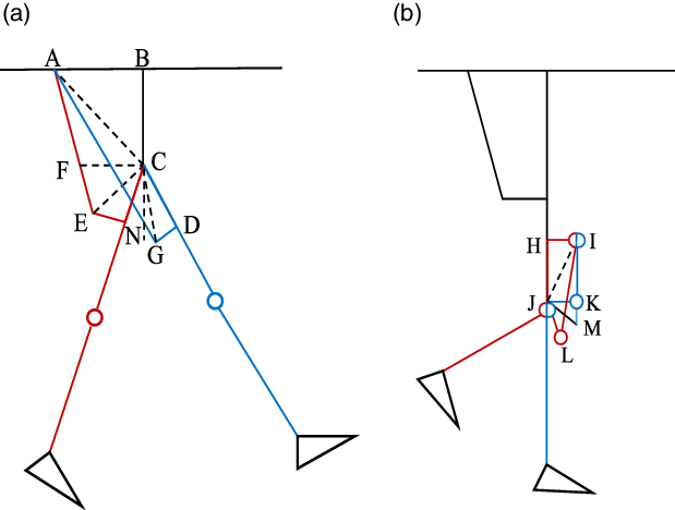
Figure 2. The schematic diagram of the exoskeleton. (a) Motion limit position diagram of hip joint; (b) Motion limit position diagram of knee joint.
Just as shown in Fig. 2(a), when the minimum flexion degree of hip joint is 40°:
 \begin{equation} AC = \sqrt{AB^{2} + BC^{2}} \end{equation}
 \begin{equation} CE = \sqrt{CN^{2} + NE^{2}} \end{equation}
 \begin{equation} \angle{ACE} = 180^{\circ}-40^{\circ}-\textrm{arcsin}\frac{AB}{AC}-\textrm{arcsin}\frac{NE}{CE} \end{equation}
 \begin{equation} AE = \sqrt{AC^{2} + CE^{2} - 2 \times AC \times CE \times \textrm{cos}\, {\angle}ACE} \end{equation}
where AE indicates that the lead screw is fully retracted. AB = 100 mm, BC = 57 mm, CD = CN = 90 mm, DG = NE = 50 mm.
When the maximum extension degree of hip joint is 35°,
 $\textit{CE} = \textit{CG}$
 \begin{equation} \angle{ACG} = 360^{\circ}-145^{\circ}-\textrm{arcsin}\frac{AB}{AC}-\textrm{arcsin}\frac{DG}{CG} \end{equation}
 \begin{equation} AG = \sqrt{AC^{2} + CG^{2} - 2 \times AC \times CE \times \textrm{cos}\, {\angle}ACG} \end{equation}
where AG means that the lead screw extends a certain distance.
 \begin{equation} \Delta{H} = AG - AE \end{equation}
where
 $\Delta{H} = 70mm$
is stroke of ball screw of hip joint.
$\Delta{H} = 70mm$
is stroke of ball screw of hip joint.
The stroke of the ball screw of the knee joint is shown in Fig. 2(b).
When the minimum extension degree of knee joint is 0°:
 \begin{equation} IJ = \sqrt{HI^{2} + HJ^{2}} \end{equation}
 \begin{equation} {\angle}IJK = 90^{\circ}-\textrm{arcsin}\frac{HI}{IJ} \end{equation}
 \begin{equation} IK = \sqrt{IJ^{2} + KJ^{2} - 2 \times IJ \times KJ \times \textrm{cos}\, {\angle}IJK} \end{equation}
where IK indicates that the lead screw is fully retracted.
When the maximum flexion degree of knee joint is 79°:
 \begin{equation} {\angle}IJL = 180^{\circ}-11^{\circ}\textrm{-arcsin}\frac{HI}{IJ} \end{equation}
 \begin{equation} IL = \sqrt{IJ^{2} + LJ^{2} - 2 \times IJ \times LJ \times \textrm{cos}\, {\angle}IJL} \end{equation}
where IL means that the lead screw extends a certain distance.
 \begin{equation} \Delta{K} = IL - IK \end{equation}
where
 $\Delta{K} = 55mm$
is stroke of ball screw of knee joint. Therefore, a lead screw with a stroke range of 100mm is selected to meet the requirements of the telescopic stroke of the ball screw
$\Delta{K} = 55mm$
is stroke of ball screw of knee joint. Therefore, a lead screw with a stroke range of 100mm is selected to meet the requirements of the telescopic stroke of the ball screw
In order to ensure that the movement mode is closer to the human movement, the linear actuator of the servo motor and ball screw was selected. The telescopic travel of the ball screw can be calculated by the limit position of each joint. For the mechanical design of the exoskeleton, the thigh rod and calf rod are adjustable, from 402 to 505 mm and 397 mm to 506 mm, respectively. The motion range of the hip joint is −38°–50.18°. The motion range of the knee joint is 0°–95.53°. In order to ensure the safety, we make the joint activity thresholds of the mechanical design larger than the actual range of motion of the human body. Through the dynamic analysis of the lower extremity exoskeleton system, the driver of hip joint and knee joint adopted the servo motor with a rated power of 400 W. The length of the ball screw is 4 mm, the rated thrust is 2000 N, the maximum linear speedup is 100 mm/s, which is sufficient for assisting people in rehabilitation training. The step function is utilized to control the speed of the ball screw. The linear motion of the ball screw is transformed into the rotational motion of the hip joint and knee joint in the sagittal plane, which approximately fits the normal gait of a human. The speed of the ball screw is input to make the lower limb exoskeleton exercise in accordance with the approximated normal human gait. The driving force of the given motion is deduced to verify whether the thrust in the previous stage is enough. The stretch and contract of thigh, calf, and waist adopted stepless adjustable mechanism. To ensure the lightweight of the robot, the carbon-fiber material and aluminum alloys are adopted. The thigh, calf, and waist are made of carbon fiber instead of the aluminum alloys. Compared to the overall structure of all aluminum alloys, the weight is reduced by 25%. This exoskeleton leg fits patients from 1.50 to 1.90 m tall, which covers more than 99% of corresponding adults, with maximum body weight of 100 kg.
3. Gait trajectory generation
The lower extremity exoskeleton robot helps patients regain their ability to walk independently. Therefore, its walking mode would be planned according to walking stability, the standard step size, leg lift height, and gait cycle of ordinary people walking. Based on the cubic spline interpolation method, a five-point segmented gait planning method is proposed to the continuous walking trajectory.
Hypothesis 1: The upper body is always vertical to the horizontal ground.
Hypothesis 2: The Z-axis coordinate condition is always constant.
Hypothesis 3: The trajectory of the swinging leg is in the sagittal plane.
Hypothesis 4: During the swing phase, the hip and knee joints of the supporting leg will not experience internal/external rotation.
Hypothesis 5: When the swing leg is landing, there will be no slipping, stepping instability, etc.
The three-point (starting moment, swinging highest point moment, and landing moment) planning method was widely applied to gait planning. Although the technique is simple, too many changes in the intermediate process between the two states and excessive amplitude are easy to ignore. The five-point segmented planning method adds two conditions: the transition from dual support phase to swing phase and the transition from swing phase to second dual support phase, making the gait planning more elaborate, just as shown in Fig. 3.
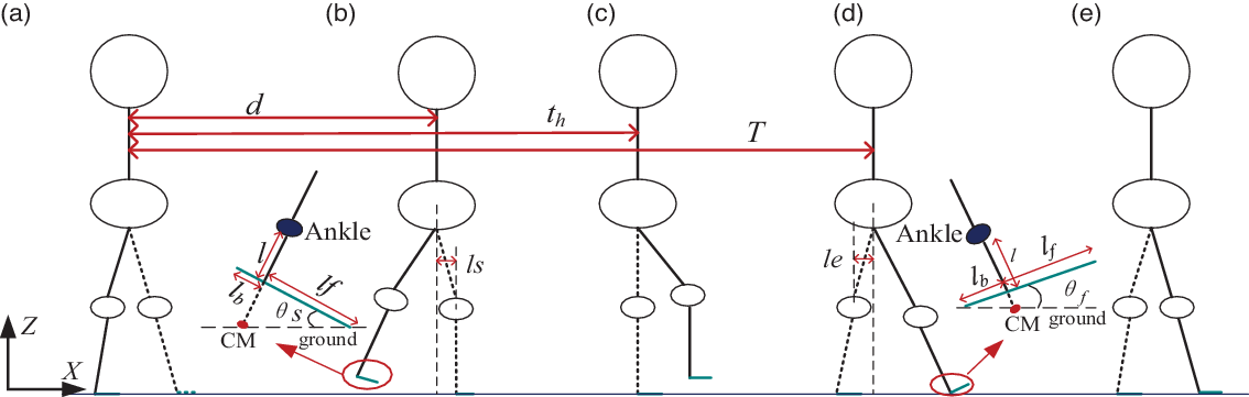
Figure 3. The state of five-point segmented gait planning method. (a). Dual support phase, (b). Initial stage of swing phase, (c). Middle stage of swing phase (d). Ending stage of swing phase (e). Second dual support phase.
3.1. Trajectory generation for ankle joint
In the swing phase, the step length of one step is set as s, and the angle between the sole of the foot and the ground is
 $\theta(t)$
.
$\theta(t)$
.
 \begin{equation} \theta(t) = \left\{ \begin{array}{c}0,t = kT \\ \theta_{s},t = kT + d \\ 0,t = kT + t_{h}\\ \theta_{f},t = (k + 1)T\\ 0,t = (k + 1)T + d \end{array} \right. \end{equation}
where k is positive integer, and k ≥ 0. T is time of one gait cycle.
During the swing phase, the posture of the swing leg is shown in Fig. 3(b)–(d). The center of mass (CM) of the sole was defined as the vertical point from the ankle joint to the foot. The length from the ankle joint to CM is represented by l. The length from the heel to CM is defined as l b . The length from the toe to CM is defined as l f .
The position of the ankle joint is
 \begin{equation} x(t) = \left\{ \begin{array}{c} ks,t = kT \\ ks+l_{f}\,(1 - \textrm{cos}\,\theta_{s}) + l\,\textrm{sin}\,\theta_{s},t = kT + d \\ ks + L_{h},t = kT + t_{h} \\ (k + l)s - l_{b}\,(1 - \textrm{cos}\,\theta_{f}) - l\,\textrm{sin}\,\theta_{f},t = (k + 1)T \\ (k + 1)s,t = (k + 1)T + d \end{array} \right. \end{equation}
 \begin{equation} z(t) = \left\{ \begin{array}{c} l,t = kT \\ l\,\textrm{cos}\,\theta_{s} + l_{f}\,\textrm{sin}\,\theta_{s},t = kT + d \\ H,t = kT + t_{h} \\ l\,\textrm{cos}\,\theta_{f} + l_{b}\,\textrm{sin}\,\theta_{f},t = (k + 1)T \\ l,t = (k + 1)T + d \end{array} \right. \end{equation}
where L h is the distance from starting point at time t h . H is the height of ankle joint.
Since at time kT and time (k+1)T+d, the supporting leg always touches the ground. Therefore, the constraint is:
 \begin{equation} \left\{ \begin{array}{c} \theta'(kT) = 0 \\ \theta'((k + 1)T + d) = 0 \end{array} \right. \end{equation}
 \begin{equation} \left\{ \begin{array}{c} x'(kT) = 0 \\ x'((k + 1)T + d) = 0 \end{array} \right. \end{equation}
 \begin{equation} \left\{ \begin{array}{c} z'(kT) = 0 \\ z'((k + 1)T + d) = 0 \end{array} \right. \end{equation}
3.2. Trajectory generation for hip joint
According to Hypothesis 2, the Z-axis coordinate of the hip joint is a constant, which is the sum of the length of the calf and the length of the thigh and the height of the ankle joint. When H is maximum, the distance traveled of the swinging leg is s/2.
 \begin{equation} x(t) = \left\{ \begin{array}{c} ks + s/4,t = kT \\ ks + l_{e},t = kT + d \\ ks + s/2,t = kT + t_{h} \\ ks + 1_{s},t = (k+1)T \\ ks + 3s/4,t = (k+1)T + d \end{array} \right. \end{equation}
where
 $s/4 < l_{e} < s/2, s/2 < l_{s} < 3s/4, l_{s}$
, represents the distance between the position of hip joint of swinging leg and the supporting leg in the initial stage of swing phase. l
e
represents the distance between the position of hip joint of swinging leg and the supporting leg in the ending stage of swing phase.
$s/4 < l_{e} < s/2, s/2 < l_{s} < 3s/4, l_{s}$
, represents the distance between the position of hip joint of swinging leg and the supporting leg in the initial stage of swing phase. l
e
represents the distance between the position of hip joint of swinging leg and the supporting leg in the ending stage of swing phase.
According to the initial speed and the final speed of the gait cycle, the constraint conditions can be obtained:
 \begin{equation} \left\{ \begin{array}{c} x'(kt) = 0 \\ x'((k + 1)T + d) = 0 \end{array} \right. \end{equation}
4. Reinforcement learning with dynamic movement primitives
4.1. Dynamic movement primitives
DMP was flexible representation for motion primitives with good stability [Reference Bottasso, Leonello and Savini20]. Any motion trajectory can be regarded as a combination of a second-order system and a nonlinear function. DMP can be described in the following form. According to the basic principle of dynamic motion primitives, in the process of trajectory learning, this method can obtain a motion trajectory that is the same as the teaching trajectory by providing teaching trajectory information, starting point value y 0 , and the final point of the trajectory g.
 \begin{equation} {\tau}z'_{\!\!t} = \alpha_{z}(\beta_{z}(g - y_{t}) - z_{t}) + R_{t} \end{equation}
 \begin{equation} {\tau}y'_{\!\!t} = z_{t} \end{equation}
 \begin{equation} {\tau}x'_{\!\!t} = -\alpha_{x}x_{t} \end{equation}
 \begin{equation} R_{t} = h_{t}^{T}(\varsigma + \varepsilon_{t}) \end{equation}
where
 $\tau$
is a scaling factor related to time. y
t
and
$\tau$
is a scaling factor related to time. y
t
and
 $y'_{\!\!t}$
are joint trajectory position and velocity. x
t
and z
t
represent the internal state. R
t
is nonlinear function which determines the shape of the trajectory. The parameters α
x
, α
z
, β
z,
and
$y'_{\!\!t}$
are joint trajectory position and velocity. x
t
and z
t
represent the internal state. R
t
is nonlinear function which determines the shape of the trajectory. The parameters α
x
, α
z
, β
z,
and
 $\varsigma$
are scale factors.
$\varsigma$
are scale factors.
 $\varepsilon_{t}$
is interference term.
$\varepsilon_{t}$
is interference term.
 $h_{t}^{T}$
is a linear function approximator, which contains Gaussian kernels
$h_{t}^{T}$
is a linear function approximator, which contains Gaussian kernels
 $\psi$
().
$\psi$
().
 \begin{equation} h_{t} = \frac{\sum\limits^{N}_{k = 1}\psi_{k}x_{t}}{\sum\limits^{N}_{k = 1}\psi_{k}}(g - y_{0}) \end{equation}
 \begin{equation} \psi_{k} = \textrm{exp}\left(-\frac{1}{2\sigma^{2}_{k}}(x_{t}-c_{k})^{2}\right) \end{equation}
where y
0
is the initial position of the trajectory. g is the final point of the trajectory. c
k
and σ
k
are the center and width of Gauss function. The parameter
 $\varsigma$
determines the shape of joint trajectory. The parameter
$\varsigma$
determines the shape of joint trajectory. The parameter
 $\varsigma$
will be adjusted by RL algorithm to update gait trajectories from y
0
to target g.
$\varsigma$
will be adjusted by RL algorithm to update gait trajectories from y
0
to target g.
4.2. Stability criteria
Stable walking of the lower limb exoskeleton is the critical research content. Zero Moment Point (ZMP) is the point where the total moment of the human-exoskeleton system is 0 during walking, and its motion trajectory can be used as the basis for stability judgment. In the walking cycle, the smallest polygon formed by the contact points between the sole and the ground is called the supporting polygon. According to the definition of ZMP, if the human-exoskeleton system can walk stably, the ZMP trajectory must always fall within the supporting polygon. To prevent the occurrence of the ZMP trajectory from falling outside the edge of the supporting polygon, a certain distance is usually left at the boundary of the supporting polygon as a stability margin.
To realize the stable walking of the lower limb exoskeleton walking aid robot, this paper abstracts the stability problem as an objective function optimization problem. The objective function is constructed with the ZMP stability margin as a parameter. The shortest distance from ZMP to the edge of the stability margin is used to build the objective function. The coordinate origin is the point where the ankle joint of the supporting foot is projected on the ground. The distance between the toe of the supporting foot and the coordinate origin is D
toe
. The distance between the heel of the supporting foot and the coordinate origin is D
heel
. The center of stability margin of the supporting foot is x
fc
= (D
toe
-D
heel
)/2. If the exoskeleton system achieves stable walking, ZMP needs to meet
 $-D_{toe} < x_{zmp} < D_{heel}$
. f(xh) is an index function reflecting the deviation of the exoskeleton from the center of stability margin.
$-D_{toe} < x_{zmp} < D_{heel}$
. f(xh) is an index function reflecting the deviation of the exoskeleton from the center of stability margin.
 \begin{equation} f(x_{h}) = (x_{zmp} - x_{fc}) \end{equation}
In this paper, a five-segment trajectory planning method is adopted, and the walking stability needs to be satisfied in each segment trajectory. In order to improve the similarity between the generation trajectory and the target trajectory, the objective function J was constructed. The smaller the J, the more stable the walking.
 \begin{equation} J = f(x_{h}) + \sum^{3}_{p = 1}M_{c}g_{p}(x_{p}) + \sum^{3}_{q =1}\frac{M_{c}}{2}h_{q}(x_{q}) \end{equation}
 \begin{equation} g_{p}(x_{p}) = \left\{\begin{array}{c} 0,x'_{\!\!h}(t_{p}) > 0 \\[5pt] \!\! |x'_{\!\!h}(t_{p})|,x'_{\!\!h}(t_{p}) < 0 \end{array} \right. \end{equation}
 \begin{align} h_{q}(x_{q}) = \left\{ \begin{array}{c} 0,-D_{toe} < x_{zmp} < D_{heel} \\[5pt] \!\! |x_{zmp}(t_{q})|,x_{zmp}(t_{q}) < -D_{toe} \\[5pt] \!\!\!\! |x_{zmp}(t_{q})|,x_{zmp}(t_{q}) > D_{heel} \end{array} \right. \end{align}
where Mc is penalty factor, gp(xp) and hq(xq) are penalty function, p, q = 1,2,3, tp and tq are corresponding time consumption of penalty function.
4.3. Reinforcement learning with trajectory optimization
At present, the method of combining RL algorithm with other technologies has a good research prospect and has been widely used in many fields. Based on the stochastic Hamilton Jacobi Bellman method and path integral strategy learning method, a probabilistic RL method was proposed to solve the statistical reasoning problem from the continuous learning and training process of the sample data. The algorithm mainly uses sample data to train and learn for solving statistical reasoning problems and has the characteristics of simplicity, stability, and strong robustness. In this paper, the RL algorithm was used to update parameter
 $\varsigma$
, which could continuously update the shape of the trajectory to reach the target trajectory.
$\varsigma$
, which could continuously update the shape of the trajectory to reach the target trajectory.
The cost function
 $S(\tau_{k})$
of DMP was defined.
$S(\tau_{k})$
of DMP was defined.
 \begin{equation} S(\tau_{k}) = \phi_{t_{N}} + \sum_{J = K}^{N - 1}r_{t_{j}} + \sum_{J = k}^{N - 1}\left\|\frac{y_{t_{j + 1}} - y_{t_{j}}}{d_{t}} - R_{t_{j}}\right\|^{2}_{H_{t_{j}}^{-1}} + \frac{\lambda}{2}\sum_{j = k}^{N - 1}\textrm{log}\|H_{t_{j}}\| \end{equation}
 \begin{equation} \phi_{t_{N}} = B_{N}(y_{t} - g)^{T} (y_{t} - g) + R_{N}y^{\prime{T}}_{t} y'_{\!\!t} \end{equation}
 \begin{equation} r_{t} = \frac{1}{2}B_{q}y^{\prime\prime{T}}_{t} y''_{\!\!\!t} + \frac{1}{2}R(\varsigma + \varepsilon_{t})^{T} (\varsigma + \varepsilon_{t}) \end{equation}
where φ
tN
denotes the terminal cost at time t
N
, B
N
and R
N
are applied for the adjustment of terminal cost, r
t
represents the current cost at time t, B
q
and R are used to change the current cost. H
t
is a scalar, and
 ${H_t} = {h_t}^{(c)T}{R^{ - 1}}{h_t}^{(c)}$
.
${H_t} = {h_t}^{(c)T}{R^{ - 1}}{h_t}^{(c)}$
.
 $\dfrac{\lambda}{2}\sum\limits_{j = i}^{N - 1} {\log \left| {{H_{tj}}} \right|}$
is a certain variable, the values of all sampling paths are same, so it could be ignored.
$\dfrac{\lambda}{2}\sum\limits_{j = i}^{N - 1} {\log \left| {{H_{tj}}} \right|}$
is a certain variable, the values of all sampling paths are same, so it could be ignored.
Then, the expression of S(
 $\tau$
i
) is updated as:
$\tau$
i
) is updated as:
 \begin{align} S(\tau_{k}) & = \phi_{t_{N}} + \sum_{N - 1}^{j = k}r_{t_{j}} + \sum_{N - 1}^{j = k}\left\|h^{T}_{t_{j}} (\varsigma_{t_{j}} + \varepsilon_{t_{j}})\right\|^{2}_{H_{t_{j}}^{-1}} = \phi_{t_{N}} + \sum_{j = k}^{N - 1}r_{t_{j}} + \sum_{j = k}^{N - 1}\frac{1}{2}(\varsigma_{t_{j}} + \varepsilon_{t_{j}})^{T}\, h_{t_{j}}\,H_{t_{j}}^{-1}\,h_{t_{j}}^{T}\, (\varsigma_{t_{j}} + \varepsilon_{t_{j}}) \nonumber \\[5pt] & = \phi_{t_{N}} + \sum_{j = k}^{N - 1}r_{t_{j}} + \sum_{j = k}^{N - 1}\frac{1}{2}(\varsigma_{t_{j}} + \varepsilon_{t_{j}})^{T}\, \frac{h_{t_{j}}h_{t_{j}}^{T}}{h_{t_{j}}^{T}R^{-1}h_{t_{j}}}(\varsigma_{t_{j}} + \varepsilon_{t_{j}}) \end{align}
According to the stochastic optimal control theory [Reference Stulp, Theodorou and Schaal21], the result of the path integral optimal problem for DMP can be expressed as:
 \begin{equation} \varsigma_{t_{k}} = \int{P}(\tau_{k})\mu_{L}(\tau_{k})d\tau_{k} \end{equation}
where
 $P({\tau _k}) = \dfrac{\exp ( - \frac{1}{\lambda }S({\tau _k}))}{\int {\exp ( - \frac{1}{\lambda}S({\tau _k}))d{\tau _k}} }$
is probability variable, and the parameter λ was used to adjust the sensitivity of the exponential function.
$P({\tau _k}) = \dfrac{\exp ( - \frac{1}{\lambda }S({\tau _k}))}{\int {\exp ( - \frac{1}{\lambda}S({\tau _k}))d{\tau _k}} }$
is probability variable, and the parameter λ was used to adjust the sensitivity of the exponential function.
 $\mu_{L}(\tau_{k}) = \dfrac{R^{-1}h_{t_{k}}h_{t_{k}}^{T}}{h_{t_{k}}R^{-1}h_{t_{k}}}\varepsilon_{t_{k}}$
is local control variable. And
$\mu_{L}(\tau_{k}) = \dfrac{R^{-1}h_{t_{k}}h_{t_{k}}^{T}}{h_{t_{k}}R^{-1}h_{t_{k}}}\varepsilon_{t_{k}}$
is local control variable. And
 \begin{equation} S(\tau_{k}) = \phi_{t_{N}} + \sum_{j = k}^{N - 1}r_{t_{j}} + \frac{1}{2}\sum_{j = k}^{N - 1}(\varsigma_{t_{k}} + \varepsilon_{t_{j}})^{T} \times \left(\frac{R^{-1}h_{tj}h_{tj}^{T}}{h_{tj}^{T}R^{-1}h_{tj}}\right)^{T}\,R\left(\frac{R^{-1}h_{tj}h_{tj}^{T}}{h_{tj}^{T}\,R^{-1}h_{tj}}\right)(\varsigma_{t_{k}} + \varepsilon_{t_{j}}) \end{equation}
The stochastic optimal control problem is solved by Eq. (37) in the whole state space. The optimal control
 $\varsigma_{tk}$
can be obtained by an iterative update procedure. With an initial value
$\varsigma_{tk}$
can be obtained by an iterative update procedure. With an initial value
 $\varsigma$
, and a random parameter
$\varsigma$
, and a random parameter
 $\varsigma + \varepsilon_{t}$
is generated at each time step. With the consideration of Eq. (36), for the sake of the iterative updates, the update rule could be written as:
$\varsigma + \varepsilon_{t}$
is generated at each time step. With the consideration of Eq. (36), for the sake of the iterative updates, the update rule could be written as:
 \begin{equation} \varsigma_{tk}^{new} = \int{P}(\tau_{k})\frac{R^{-1}h_{t_{k}}h_{t_{k}}^{T}(\varsigma + \varepsilon_{t_{k}})}{h_{t_{k}}^{T}\,R^{-1}h_{t_{k}}}d\tau_{k} = \int{P}(\tau_{k})\frac{R^{-1}h_{t_{k}}\,h_{t_{k}}^{T}\varepsilon_{t_{k}}}{h_{t_{k}}^{T}\,R^{-1}h_{t_{k}}}d\tau_{k} + \frac{R^{-1}h_{t_{k}}\,h_{t_{k}}^{T}\varsigma_{t_{k}}}{h_{t_{k}}^{T}\,R^{-1}h_{t_{k}}} = \zeta\!\varsigma_{t_{k}} + \frac{R^{-1}h_{tj}\,h_{tj}^{T}}{h_{tj}^{T}\,R^{-1}h_{tj}}\varsigma \end{equation}
where
 $\zeta\!{\varsigma _{{t_k}}} = \int {P({\tau _k})} \dfrac{{R^{ - 1}}{h_{{t_k}}}h_{{t_k}}^T{\varepsilon _{{t_k}}}}{h_{{t_k}}^T{R^{ - 1}}{h_{{t_k}}}}d{\tau _k}$
,
$\zeta\!{\varsigma _{{t_k}}} = \int {P({\tau _k})} \dfrac{{R^{ - 1}}{h_{{t_k}}}h_{{t_k}}^T{\varepsilon _{{t_k}}}}{h_{{t_k}}^T{R^{ - 1}}{h_{{t_k}}}}d{\tau _k}$
,
 $\varsigma _{_{{t_k}}}^{new}$
is not time-independent. For each time step t
k
, a new optimization parameter
$\varsigma _{_{{t_k}}}^{new}$
is not time-independent. For each time step t
k
, a new optimization parameter
 $\varsigma _{_{{t_k}}}^{new}$
would be obtained. However, the time-independent parameter ς
new
was needed, the parameter
$\varsigma _{_{{t_k}}}^{new}$
would be obtained. However, the time-independent parameter ς
new
was needed, the parameter
 $\varsigma_{tk}^{new}$
was averaged over time t
k
.
$\varsigma_{tk}^{new}$
was averaged over time t
k
.
 \begin{equation} \varsigma^{new} = \frac{1}{N}\sum_{t = 0}^{N - 1}\varsigma^{new}_{t_{k}} = \frac{1}{N}\sum_{t = 0}^{N - 1}\zeta\!\varsigma_{t_{k}} + \frac{1}{N}\sum_{t = 0}^{N - 1}\frac{R^{-1}\,h_{t_{k}}\,h_{t_{k}}^{T}}{h_{t_{k}}^{T}\,R^{-1}\,h_{t_{k}}}\varsigma_{t_{k}} \end{equation}
The parameter
 $\varsigma^{new}$
includes two parts. The first term is the average value of
$\varsigma^{new}$
includes two parts. The first term is the average value of
 $\zeta\!\varsigma_{t_{k}}$
. It reflects the useful information obtained from the mixed noise information. The second term is the interference term, which causes the loss of parameter
$\zeta\!\varsigma_{t_{k}}$
. It reflects the useful information obtained from the mixed noise information. The second term is the interference term, which causes the loss of parameter
 $\zeta$
. When the average value of
$\zeta$
. When the average value of
 $\zeta\!\varsigma_{t_{k}}$
becomes 0, the convergence will be realized. Therefore, the second term does not need to further update. The second term should be eliminated. The parameter
$\zeta\!\varsigma_{t_{k}}$
becomes 0, the convergence will be realized. Therefore, the second term does not need to further update. The second term should be eliminated. The parameter
 $\varsigma^{new}$
is updated to:
$\varsigma^{new}$
is updated to:
 \begin{equation} \varsigma^{new} = \frac{1}{N}\sum_{t = 0}^{N - 1}\zeta\!\varsigma_{t_{k}} + \frac{1}{N}\sum_{t = 0}^{N - 1}\varsigma_{t_{k}} = \frac{1}{N}\sum_{t = 0}^{N - 1}\zeta\!\varsigma_{t_{k}} + \varsigma \end{equation}
where
 $\varsigma^{new}$
is generated by the averaged value of
$\varsigma^{new}$
is generated by the averaged value of
 $\zeta\!\varsigma_{t_{k}}$
, and the current value of
$\zeta\!\varsigma_{t_{k}}$
, and the current value of
 $\varsigma$
was added in each iteration.
$\varsigma$
was added in each iteration.
The update of parameter
 $\varsigma$
is the most important part of the improved strategy algorithm, and it will affect the shape of the trajectory. The big difference between improved strategy and path integrals is using the combination of RL-based DMP and path integrals, where RL-based DMP can guarantee the stability of the system. The update rule of strategy improvement with path integrals is as follows. The parameters
$\varsigma$
is the most important part of the improved strategy algorithm, and it will affect the shape of the trajectory. The big difference between improved strategy and path integrals is using the combination of RL-based DMP and path integrals, where RL-based DMP can guarantee the stability of the system. The update rule of strategy improvement with path integrals is as follows. The parameters
 $\varsigma$
is mixed with noise interference; therefore, the noise interference
$\varsigma$
is mixed with noise interference; therefore, the noise interference
 $\varepsilon_{t}$
was added to the parameter
$\varepsilon_{t}$
was added to the parameter
 $\varsigma$
in DMP algorithm. While learning and updating the parameter
$\varsigma$
in DMP algorithm. While learning and updating the parameter
 $\varsigma$
, the updated result will lead to changes in the trajectory, and the corresponding cost function S() also changes. As the number of updates increases, the cost function S() gradually decreases and stabilizes to minimum value, and finally, the DMP system tends to be a noiseless system.
$\varsigma$
, the updated result will lead to changes in the trajectory, and the corresponding cost function S() also changes. As the number of updates increases, the cost function S() gradually decreases and stabilizes to minimum value, and finally, the DMP system tends to be a noiseless system.
4.4. Segmented multiple-DMP trajectory learning method
When the DMP parameter values y o and g are same, the learning trajectory is always a straight line, and the DMP method is invalid. However, the motion trajectory of the joint tends to be a sine function, and it is very likely that the values of y 0 and g are the same. Therefore, this paper proposed a segmented multiple-DMP trajectory learning method. Combined with five-point segmented gait planning method, the learned trajectory is divided into multiple monotonic trajectories. Because the starting value and target value of each segment of the learning trajectory after segmentation are not equal, the DMP method will not invalid. The specific steps of the segmented multiple-DMP trajectory learning method are as follows: The target trajectory was divided into multiple monotonous trajectories with five key moments as the dividing points. The target trajectory is divided into four segments. To learn each monotonous trajectory, set new starting value and target value, respectively. The target value of the previous segment is equal to the starting value of the following segment of the trajectory. The initial value of each segment of the target trajectory can be expressed as:
 \begin{equation} Y = [y_{KT}(k = 0, y_{KT} = y_{0}), y_{KT + d}, y_{KT + t_{h}}, y_{(k + 1)T}, y_{(k + 1)T + d}] \end{equation}
The target value of the target trajectory can be expressed as:
 \begin{equation} G = [y_{KT + d}, y_{KT + t_{h}}, y_{(k + 1)T}, y_{(k + 1)T + d},g] \end{equation}
The values of adjacent time points must be different, so the trajectory learning problem of g = yo is transformed into a multi-segment trajectory learning problem of g ≠ yo .
In the multi-DMP sequence, the target parameter g of a DMP is used as the starting parameter of the next DMP, and it can affect the cost of subsequent DMP. It is equivalent to using the cost of the current DMP and the cost of the remaining DMP in the sequence to optimize the shape parameter
 $\varsigma$
.
$\varsigma$
.
The cost function of multiple-DMP is defined as
 \begin{equation} S\left(\Pi_{c}\right) = \sum_{j = c}^{C}S(\tau_{t_{0}}^{j}) \end{equation}
where
 $\Pi_{c}$
denotes the c section trajectory in the C sequences.
$\Pi_{c}$
denotes the c section trajectory in the C sequences.
 $S(\tau_{t_{0}}^{j})$
denotes the cost function of the j-th trajectory in C sequence at time t
0
.
$S(\tau_{t_{0}}^{j})$
denotes the cost function of the j-th trajectory in C sequence at time t
0
.
 $s(\Pi_{c})$
denotes the total cost of the current trajectory and all subsequent sequential trajectories.
$s(\Pi_{c})$
denotes the total cost of the current trajectory and all subsequent sequential trajectories.
The parameter update rule of multi-DMP sequence is similar to that of single DMP, and the specific rules are as follows:
 \begin{equation} S(\tau_{t_{j, N}}) = \sum_{j = 0}^{N}r_{t_{j}} + \varsigma_{t_{j}}^{T}\,R\varsigma_{t_{j}} \end{equation}
 \begin{equation} S\left(\Pi_{c, k}\right) = \sum_{i = c}^{C}S(\tau_{t_{0},k}^{j}) \end{equation}
 \begin{equation} P\left(\Pi_{c, k}\right) = \frac{\textrm{exp}\left(\left(-\dfrac{1}{\lambda}S\left(\Pi_{c, k}\right)\right)\right)}{\sum\limits_{l = 1}^{K}\textrm{exp}\left(\left(-\dfrac{1}{\lambda}S\left(\Pi_{c, l}\right)\right)\right)} \end{equation}
 \begin{equation} \zeta\!\varsigma_{c} = \sum_{k = 1}^{K}P\left(\Pi_{c, k}\right)\varepsilon_{k}^{\varsigma{c}} \end{equation}
 \begin{equation} \varsigma_{c}^{new} = \varsigma_{c} + \zeta\!\varsigma_{c} \end{equation}
where Eq. (44) is the cost function of a certain trajectory; Eq. (45) is the calculation of the cost of all sequences.
5. Experimental verification
5.1. Experimental platform
This paper describes a novel gait trajectory planning method based on multiple-DMP and RL algorithm for lower exoskeleton robot. In Fig. 4, the exoskeleton robot system consists of three levels of architecture, including an upper-level controller, a lower limb exoskeleton robot, and a low-level controller. The upper-level control system consists of the data processor Raspberry Pi, which is used to process data collected from encoders (AD36/1217AF. ORBVB, Hengstler, Germany). The joint movement data of the hip joint were acquired by encoder 1 encoder 2, encoder 3, and encoder 4 together. The low-level controller controls the robot to perform trajectory. The communication mode between the upper-level and the low-level controller is parallel port communication. The low-level controller is used to control the motors through the Controller Area Network (CAN) Fieldbus. The experiment was conducted in Tianjin Key Laboratory for Integrated Design & Online Monitor Center. Two healthy male subjects (subject A and subject B) were recruited for the experiment, with averaged age 24 years old, averaged height 174 cm, averaged weight 71.73 kg. The subjects were instructed to perform normal walking with exoskeleton on the ground. For safety reasons, there are two levels of safety measures taken. Firstly, if the angle of the exoskeleton is greater than the allowable value (The motion range of the hip joint is −38°–50.18°. The motion range of the knee joint is 0°–95.53°), the exoskeleton will be forced to stop moving by software. Besides, the subjects could cut off the power through the emergency switch button if they need to do it at any time, just as shown in Fig. 5.

Figure 4. Prototype of the proposed exoskeleton robot.

Figure 5. Human experiment.
5.2. Parameters setting
The time of dual support phase d is 0.2 s. The one-step length s is 0.6 m. The maximum height of ankle joint H is 0.25 m, and the elapsed time t
h
is 0.5 s. The parameters l
b
, l, l
s,
and l
e
are set as 0.06, 0.1, 0.4, and 0.2 m, respectively. The length of calf is 0.3 m. The length of thigh is 0.5 m. The height of hip joint is 0.7 m. The velocity of horizontal hip of subject A and subject B is 0.8 m/s and 0.67 m/s, respectively. The parameters of DMP equation are
 $\alpha$
z
= 20,
$\alpha$
z
= 20,
 $\beta$
z
= 20, τ = 0.2. The parameters of cost function are BN =
$\beta$
z
= 20, τ = 0.2. The parameters of cost function are BN =
 $10^{-5}$
, R =
$10^{-5}$
, R =
 $10^{-5}$
, B
N
= 10, R
N
= 25. The parameters of stability criteria are D
toe
= 0.15 m, D
heel
= 0.1 m, M
c
= 300.
$10^{-5}$
, B
N
= 10, R
N
= 25. The parameters of stability criteria are D
toe
= 0.15 m, D
heel
= 0.1 m, M
c
= 300.
5.3. Experimental results
In the experiment, the trajectory learning of all joints of the lower limb exoskeleton is updated at the same time. The number of updates is set to 70. After each update, DMP generates the required joint trajectory. Then, the actual joint trajectory is obtained. The data from the actual joint trajectory are used as the value of the RL algorithm to calculate the corresponding cost, and the shape and target parameters are updated. After the shape and target parameters are updated, the multiple-DMP algorithm is used to generate a new desired joint trajectory for the lower limb exoskeleton.
The experimental results are presented in Figs. 6–8. Figures 6 and 7 show the actual learning trajectories of the two joints in the lower exoskeleton. In order to show the effect of learning clearly, six groups of data are obtained by sampling data every ten times. Each joint trajectory is composed of four sequential segments. Due to the environmental disturbance, the learning trajectory at the initial time has a larger state error. Although the subjects’ movement and speed were inconsistent, the stable convergence of the two tests is achieved through continuous learning. The experimental results show that the reinforcement learning algorithm can well suppress uncertainty and interference. After 30 iterations, with the increase of the number of updates, the amplitude is gradually stable and convergent, which verifies the learning performance of the reinforcement learning algorithm, and shows that the joint trajectory is convergent. The change in the total cost value of all trajectories is shown in Fig. 8. The amplitude tends to stabilize and converge as the number of updates increases, which verifies the validity and superiority of the proposed method. The video capture of the human experiment is shown in Fig. 9. The time of a complete gait cycle of subject A is 1.5 s. The experiment demonstrates that the exoskeleton robot can effectively assist the human body to realize stable walking.

Figure 6. Actual learning trajectories of joints of subject A. (a) Trajectory of hip joint. (b) Trajectory of knee joint.

Figure 7. Actual learning trajectories of joints of subject B. (a) Trajectory of hip joint. (b) Trajectory of knee joint.

Figure 8. Cost during reinforcement learning of subject A.

Figure 9. The video snapshot of subject A’s experiment.
5.4. Stability analysis
Based on the D’Alembert’s principle, when the exoskeleton and human body were regarded as the multi links systems, the ZMPs could be calculated by Eqs. (49) and (50) [Reference Aphiratsakun, Chairungsarpsook and Parnichkun32]. So the ZMP positions of the exoskeleton and human body in the coordinate system could be determined when walking.
 \begin{equation} x_{zmp} = \frac{\sum_{i}m_{i}(z''_{\!\!\!i} + G_{g})x_{i} - \sum_{i}m_{i}x''_{\!\!\!i}z_{i}}{\sum_{i}m_{i}(z''_{\!\!\!i} + G_{g})} \end{equation}
 \begin{equation} y_{zmp} = \frac{\sum_{i}m_{i}(z''_{\!\!\!i} + G_{g})y_{i} - \sum_{i}m_{i}y''_{\!\!\!i}z_{i}}{\sum_{i}m_{i}(z''_{\!\!\!i} + G_{g})} \end{equation}
where Gg is gravitational acceleration. (x i , y i , z i ) locates the center of mass of link-i, and m i represents the mass of link i.
Only the Sagittal plane was considered, and the position trajectories of body ZMP and exoskeleton ZMP are shown in Fig. 10. From the graph, we could see the ZMP of exoskeleton could track the wear’s ZMP well. And there is no greater ZMP gap caused by the interference. The whole system could run stably and effectively.

Figure 10. The position trajectories of body ZMP and exoskeleton ZMP.
6. Conclusion
This paper proposes a new method that can help the human body walk stably with the lower limb exoskeleton robot. The mechanical structure and robot system of the 6-DOFs exoskeleton robot is introduced. A new five-point walking trajectory planning method for the lower limb exoskeleton robot is proposed. The novel stability criteria of human-exoskeleton system are based on ZMP. And we could see the ZMP of exoskeleton could track the wear’s ZMP well from experimental results. Besides, the multiple DMP strategy based on reinforcement learning is used to transform the trajectory of task space into the trajectory of angle space, which reduces the influence of external systems and various disturbances. It can be seen from the experiment that with the participation of multiple-DMP algorithm based on RL algorithm, the trajectory of the exoskeleton robot could be continuously adjusted to track the target trajectory smoothly. The current research content is mainly for simple locomotion scenes. Future work will consider the concept of the adaptive training strategy to strengthen the universality of the exoskeleton robot.
Consent to Publish
The work described has not been submitted elsewhere for publication, in whole or in part, and all the authors listed have approved the manuscript that is enclosed.
Authors Contributions
All authors have made substantial contribution. The first author Peng Zhang designed the experiment scheme, analyzed the experimental results, and wrote the paper. Corresponding author Junxia Zhang modified the paper.
Funding
This work was supported in part by the Hundred Cities and Hundreds Parks Project-Key Nutrition and Health Technology and Intelligent Manufacturing(21ZYQCSY00050).


