Introduction
Microwave (MW) sensors can be listed such as special transmission sensors, guided wave transmission sensors, free-space transmission sensors, time domain reflectometry (TDR) and tomographic sensors. In some industrial applications, for instance, strength grading and drying, it is critical to investigate the moisture content, density or even check if there are defects (hollow) in wood. The dielectric constant and conductivity of materials were studied in many applications, especially when MWs were employed and used for wood characterization [Reference Deshours, Alquié, Kokabi, Rachedi, Tlili, Hardinata and Koskas1–Reference Soffiatti, Max, Silva and de Mendonça4].
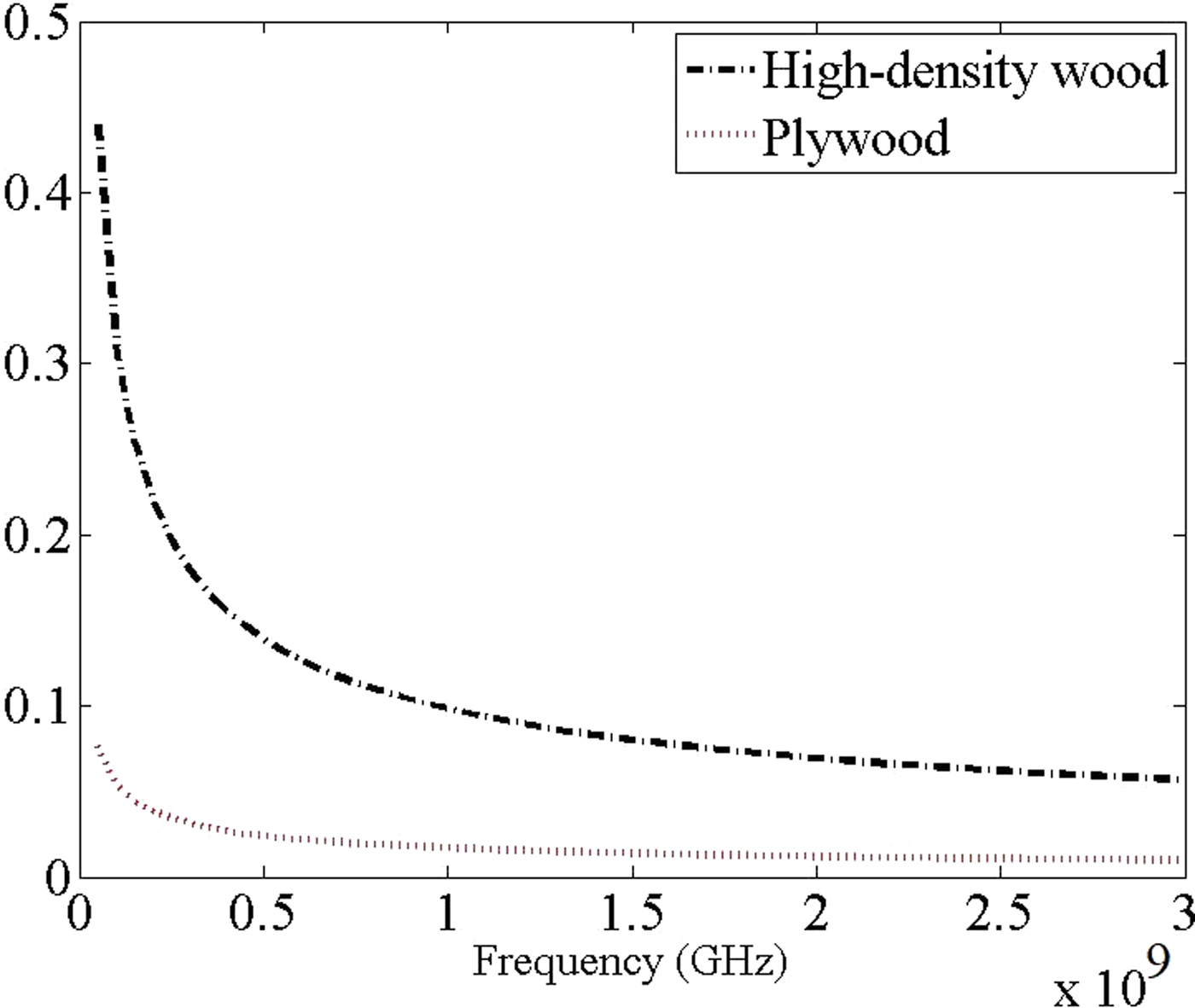
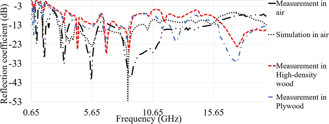
MWs are known as a non-destructive method to detect defects in wood [Reference Hansson, Lundgren, Antti and Hagman5]. It was clearly presented that wood's electrical properties such as the dielectric constant were highly affected by parameters like frequency, temperature, moisture content, and density. The dielectric properties of wood and oil palm trunk (OPT) were presented in different features at both THz and MW frequency range, respectively, in [Reference Suslyaev, Kochetkova, Dunaevskii and Dorozhkin6, Reference Jie, Abdullah, Yusof and Abbas7]. For instances, the dielectric measurement was performed in the THz frequency range for both parallel and perpendicular polarization to the fiber direction of wood. A weak reduction in the real part of the permittivity and an ignorable increase for the imaginary part of permittivity were noticed when it was in parallel. Moreover, for the perpendicular direction, the real part reduced till 250 GHz and then had a slight enhancement until 500 GHz. In addition to that, dielectric properties of OPT core were evaluated using an open-ended coaxial probe method applying in three directions as radial, tangential, and cross-section in the frequency range of 0.5–3.5 GHz. When the frequency was increased from 1 to 3 GHz, the dielectric constant decreased for all the fiber directions. Besides, their results showed that the electric field of MW was affected when the OPT core biomass interacted with electromagnetic waves [Reference Wun, Abdullah, Yusof and Abbas8] checked the other type of biomass such as rubber wood, softwood included Black spruce, Balsam fir and Tamarak, empty fruit bunch of oil palm, oil palm shell, oil palm fiber, biochar from oil palm shell, green pea flour, lentil flour, soybean flour, and the same tendency of dielectric constant changes in terms of frequency was noticed. Hence, these waves were highly used in medical imaging (MI) [Reference Salvadè, Pastorino, Monleone, Randazzo, Bartesaghi, Bozza and Poretti9] and MW tomography (MWT) [Reference Hafiz, Rahiman, Tan, Kiat, Ping and Abdul10] applications since there were non-invasive. The measured dielectric properties of the applied samples (high-density wood and plywood) using the Keysight 85070D dielectric probe depicts in Fig. 1. This measurement confirmed that the same trend followed in the sample's dielectric properties used in this work. Furthermore, the penetration depth of the electromagnetic wave at the wavelength of the incident field in meter is presented in Fig. 2. It is illustrated that the high-density wood shows better penetration since its conductivity is less than the plywood. Besides, penetration depth follows the same trends for both samples as it decreases with frequency.
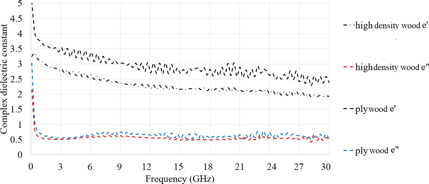
Fig. 1. Dielectric measurement of the samples.

Fig. 2. Penetration in both high-density wood and plywood (in meter).
MWT uses tomographic sensors (like antennas in this paper to send and receive the signals) and electromagnetic principles in imaging (to investigate the variation of electric and magnetic fields around the sample) and it showed more advantages in comparison with other methods like Electrical Capacitance Volume Tomography (ECVT) (MW imaging (MWI) showed more promising performances and advantages in comparison with the ECVT and the other techniques presented in Table A1 in Appendix. According to the references presented in this table, the MWI technique has better outcomes in terms of the speed and none invasive effects on the body as compared with others presented) [Reference Noghanian, Sabouni, Desell and Ashtari11].
A MWT system usually uses three major parts, which consists of a sensing system (transmitting and receiving antennas), an interfacing (signal conditioning), and an image reconstruction algorithm (an algorithm to construct the image) [Reference Wahad, Rahim, Rahiman, Aw, Yunus, Goh and Rahim12]. Moreover, MWT was applied in many applications such as MI in breast cancer imaging [Reference Eesuola, Chen and Tian13], geographical prospecting like finding mines [Reference Vertiy, Gavrilov, Voynovskiy, Aksoy and Salman14], agriculture like the imaging of defects in wood [Reference Pastorino, Salvad, Monleone, Bartesaghi, Bozza and Randazzo15], and wood characterization [Reference Pastorino, Randazzo, Fedeli, Salvadè, Maffongelli, Monleone and Lanini16]. The geophysical imaging of root zone, trunk, and moisture heterogeneity was performed in [Reference Al Hagrey17]. Another paper worked on the MWT to inspect the wood [Reference Boero, Fedeli, Lanini, Maffongelli, Monleone, Pastorino, Randazzo, Salvadè and Sansalone18]. In addition to that, the imaging of wood not only used for MW region but also for a higher range like THz in [Reference Koch, Hunsche, Schuacher, Nuss, Feldmann and Fromm19] and even MWI of wood materials helped to inspect the damage caused by earthquake presented in [Reference Liu, Koyama, Zhu, Liu and Sato20]. The antennas presented in [Reference Liu, Koyama, Takahashi and Sato21, Reference Cetin, Benedickter and Leuchtmann22] obtained a narrow BW, and their antenna dimensions were larger in comparison with the antenna presented in this paper.
As aforementioned, one part of MWT system is the transmitter and receiver which are antennas. Having a wide BW in MWT are helpful for artifact removal and better resolution [Reference Ahadi, Binti, Isa, Bin Saripan, Zuha and Hasan23], ultra-wideband (UWB) antennas can be a useful choice. Based on the Federal Communication Commission, UWB antennas are licensed to use a frequency range from 3.1 to 10.6 GHz, whilst in some application's higher frequency bands (mm-waves/THz) were exploited [Reference Chen, Chen, Tseng, Lu, Kuo, Fu, Lee, Tsai, Huang, Chuang, Hwang and Sun24]. Many types of UWB antennas exist with different shapes and characteristics such as planar UWB antennas, printed (2D) and over metal plate UWB antennas, bowl shape, leaf shape, U-shape antennas, and C-shape antennas [Reference Cicchetti, Miozzi and Testa25]. For instance, elliptical patches permit the operational bandwidth (BW) to span over a UWB range. In some cases, the radiating patch was optimized to improve the Radar Cross Section, while two slots were cut from the patch to obtain a good radiation performance and enhance impedance matching of the designed antenna. One of the benefits of an UWB antenna is to have broad BW, which assists in giving a high resolution for detecting small differences in the medium under test or even detecting a small movement of the chest when we breathe [Reference Bernardi, Cicchetti, Pisa, Pittella, Piuzzi and Testa26]. Furthermore, for MWI applications, when the working BW is wide enough, high resolution in image reconstruction and clutter removal are achievable. Besides, to decrease the effect of clutter on the image and reduce the number of imaging artefacts, more antennas to receive more scattered signals from healthy tissue and unhealthy one can be helpful; thus, the antenna dimension is better to be small [Reference Ahadi, Binti, Isa, Bin Saripan, Zuha and Hasan23]. In addition to that, MWT is beneficial in comparison with other methods in terms of having high-resolution, not harmful for the human body and giving 3D images of data compared with other methods (Table A1, Appendix) [Reference Min27] applied two antennas, one circular-edge antipodal Vivaldi antenna and one corrugated balanced antipodal Vivaldi antenna. Afterward, the s-parameters, radiation characteristics of antenna like gain, transmitted and received signals of arrays antenna were investigated in the range of 3.1–10.6 GHz. The results showed improvement in feasibility of UWB imaging of the wood slice. [Reference Liu, Koyama, Zhu, Liu and Sato20] Presented a polarimetric radar system for sensing the concealed wood-frames damaged by earthquakes. This system employed an antenna array consisting of four linearly polarized Vivaldi antennas recording full-polarimetric radar echoes in an UWB ranging from 1 to 20 GHz. Afterwards, several surveys were used on damaged wooden wall specimens in laboratory. The experiment results indicated that the high-frequency radar waves could penetrate the wooden walls. The shape and orientation of the wooden members have shown a great sensitivity to the radar polarization. It is concluded that radar polarimetry could provide much richer information on the condition of concealed wooden structures than the conventional single-polarization subsurface penetrating radar. In [Reference Pastorino, Randazzo, Fedeli, Salvadè, Maffongelli, Monleone and Lanini16] two log-periodic UWB antennas with dimensions of 300 mm × 210 mm were used for imaging of the wood slog. They were able to directly provide images of the distributions of the dielectric properties inside the samples under test. The obtained results confirmed that MWI successfully applied for creating maps of the internal structure of wood samples and they allow to extract information about the health and quality of the wood. Presently, the system has been proven to be able to quantitatively reconstruct targets whose maximum dimensions are about 0.1 m in green condition and about 0.25 m in dry conditions. In another design, a non-resonant UWB antenna worked based on the quad-ridged horn design [Reference Cetin, Benedickter and Leuchtmann22]. It was dual-polarization and operational in the frequency range of 0.7–10 GHz. A homogenous wooden slab used and its damping S 21 was investigated in desired distance and frequency to check how the S 21 was changing. They showed that simulations were reliable and could be used in the prediction of transmission through the wall.
In this paper, measurements are performed on high-density wood, soft plywood, and in air. Although this might not be as realistic as the work presented in [Reference Schajer and Orhan28–Reference Rattanadecho31], it can still be considered as a promising method in the MWI of wood in terms of the antennas' and system dimensions, and not being destructive (recently, similar systems such as Gamma scorpion and ECTV shown in Table A1 Appendix, applied bulky systems with large dimension antennas and were destructive like X-ray and Gamma. But the proposed system is smaller with high gain and broad BW and also beneficial for the detection of defects in wood).
Since the number of antennas is directly related to the imaging accuracy, the UWB antenna is better to be low in profile. The best choice for this purpose is the planar antennas. The key challenges in MWT of wood can be listed as follows (the advantages and disadvantages of the methods are presented in Table A1, Appendix): dimensions of the applied antennas and systems, and the ability to obtain 3D images with high resolution. Many techniques were used in imaging of wood other than MWI such as ECVT [Reference Fei, Qussai and Liang32], High-Resolution X-Ray Computed Tomography (HRXCT) [Reference Mayo, Chen and Evans29], or Gamma scorpion [Reference Abdullah, Hassan, Shari, Mohd, Mustapha, Mahmood, Jamaludin, Ngah and Hamid33], Electric ring electrode array, and Seismic tomography of trunks [Reference Al Hagrey17]. But, each of these methods used for imaging of wood showed drawbacks that affected the imaging of wood in terms of the inadequate spatial resolution and is not portable. For instances, ECTV demonstrated the disadvantages such as inadequate spatial resolution it can provide, the measurement resolution that is dependent on ECT sensor designs and image reconstruction, and the highly nonlinear reconstruction problem is still considered as the main obstacle to increase resolution, and the nonlinearity of the problem is increased substantially (Table A1, Appendix).
Recently, many kinds of microstrip antennas were simulated and designed for imaging and tomography of the breast to detect tumors which had individual specifications. In [Reference Mohammed, Abbosh and Sharpe34], due to the small dimensions of the antenna, it could not cover the entire BW. Furthermore, the proposed antenna obtained a wider BW and more stable field pattern than that presented in [Reference Latif, Flores-Tapia, Pistorius and Shafai35]. In [Reference Gibbins, Klemm, Craddock, Leendertz, Preece and Benjamin36], an antenna with packed dimensions benefited from a wide slot designed to work as a UWB antenna. Besides, the transmission response of the proposed antenna is about 5 dB in the simulation and <10 dB in measurement across most of the BW. A miniaturized antenna was presented in [Reference Sugitani, Kubota, Toya, Xiao and Kikkawa37] but the reflection coefficient level was low within the acceptable BW. In [Reference Jafari, Deen, Hranilovic and Nikolova38], a bigger UWB antenna showed a smaller operating BW.
The proposed antenna has smaller dimensions as compared with the other recent and similar works; thus, when the antenna is small, more antennas can be used to send and receive more signals and better clutter removal in imaging. Furthermore, it has been shown that, with proper antenna design and signal processing, the clutters due to scatters and tag's antenna structural backscattering can be easily removed [Reference Guidi, Dardari, Roblin and Sibille39]. In addition to that, Radar-based method used several antennas to examine the breast with low power UWB pulses. The scattered fields were received by the same or different antennas. A prerequisite for MW radar techniques is a suitable transmitter/receiver like UWB antenna. To maximize the number of antennas to receive more data from the scattered signal, the size of the antenna should be as small as possible. Planar antennas are the best option for this purpose. This allows us to have more antennas to collect more scattered signals from the breast, and as a result, it decreases clutter in the image [Reference Ahadi, Isa, Iqbal Saripan and Hasan40, Reference Jafari, Jamal Deen, Hranilovic and Nikolova41]. In another work, several MW sensors (transmitters and receivers) were distributed on a circular region that may surround the object under investigation to measure scattered fields. Each sensor is alternatively activated as a transmitter, and the received signal at the rest of the sensors is captured, thus allowing to use information from all directions in the reconstruction procedure. UWB signals are proposed as illuminating signals which can provide enhanced image resolution and more clutter rejection as compared with mono-frequency reconstructions [42]. For imaging of wood, clutter and artifact can be defined as the effect of wood's crust (skin) or vascular tissues of heterogeneous in the wood sample.
This paper is divided into four sections. The first section presents an introduction to the present UWB antennas and MWI in different environments and applications. The proposed antenna's design steps are demonstrated and then its characteristics are investigated in the section Antenna design. Then, the simulated and measurement results are illustrated in the section Simulated and experimental results. Finally, the paper concludes in the section Conclusion.
Antenna design
In MWI, the UWB antennas should be able to send and receive the signals and produce an acceptable image with high resolution. The image resolution has a direct relation with operating frequency and BW of the antenna. Hence, a higher image resolution is obtained when both the working BW and the operating frequency are high as well. However, an increase in the frequency leads to less increase in wood since the wavelength is decreased.
The proposed UWB antenna is designed to radiate and receive UWB impulses with frequency content from about 2.68 GHz to about 16 GHz. To simulate the proposed UWB antenna, an elliptical shape patch, stub, shorting pins, and a truncated ground are used and then fed by the transmission line (TL) through a SMA port. A coaxial feed line connected to the SMA port delivers a UWB impulse to a TL at the base of the antenna. Thus, the proper dimension of the TL (width and length) helps to avoid spurious currents on the sheath of the coaxial feed line that could cause distortions in the antenna pattern and undesired variations in overall system performance and matching.
In designing the procedure of the antenna, patch, TL, and substrate dimensions, the ground length (these features are important to make the initial UWB antenna), and the loading of the antenna with stub (the long stub connected to the junction), slots cut form the patch and the ground, and strips at the back play important role in order to get an UWB antenna with wide BW and high performances (Fig. 6 shows the current distribution of the proposed antenna around the lower and higher end of the UWB). The design steps can be explained as follows: first, a conventional elliptical patch antenna is designed at center frequency of 10 GHz and its radiation characteristics (reflection coeffecient, BW, radiation efficiency, directivity, and gain) are investigated (The patch and ground dimensions are optimized, as the ground length should be λ/8). The operation frequency calculation equations of the antenna as a function of the patch width along with its length are given in [Reference Kumar and Saxena43, Reference Tilanthe, Sharma and Bandopadhyay44]. Besides, the length of the patch (major axis of the elliptical patch) gives the low end of the ultra-wide BW and the width (minor axis of the elliptical patch) helps in wider impedance BW. The conventional UWB antenna at this center frequency achieved the lower end at 3.2 GHz and the first pole at 3.8 GHz.
After achieving the first pole and the lower end of the ultra-wide BW, the antenna is loaded by a stub connected to the junction between the patch and the TL to resonate at the ISM frequency band and shift the working band to the lower band as well. The length is chosen based on the desired low resonant frequency and the position of this stub according to the surface current around the patch and the stub (Fig. 5 shows the current distribution of the proposed antenna around the long stub connected to the junction). Besides, after adding the stub to the patch, the surface wave around the junction and the coupling are enhanced negatively; hence, the ground cut and chamfered at the middle compensate this drawback, which degrades both the radiation efficiency and the reflection coefficient level. Apart from cutting the ground at the middle, another way to decrease the surface wave and coupling is to cut a slot from the patch to separate the stub from the patch, which reduces the surface waves. Lack of this slot causes a reduction in the radiation efficiency and the reflection coefficient matching level. Moreover, it produces another resonance in the lower band (0.9 GHz) (A Vivaldi UWB antenna was used for inspecting a wooden frame for the range of 1–20 GHz). Thus, it is tried to have a resonance after 1 GHz without enhancing the antenna dimensions. Besides, the antenna can be useful for both ISM (0.9 GHz) and L-band (1.6 GHz) [Reference raj, Rajoriya and Singhal45]. Besides, the antenna behaves as a quarter wave monopole antenna.
Then, the antenna is loaded by one strip line at the back with the length of L load to shift the working BW to a lower band and to suppress further the stop-band that occurred. Finally, to have a high-performance antenna, the antenna design parameters should be optimized at each step of the antenna design.
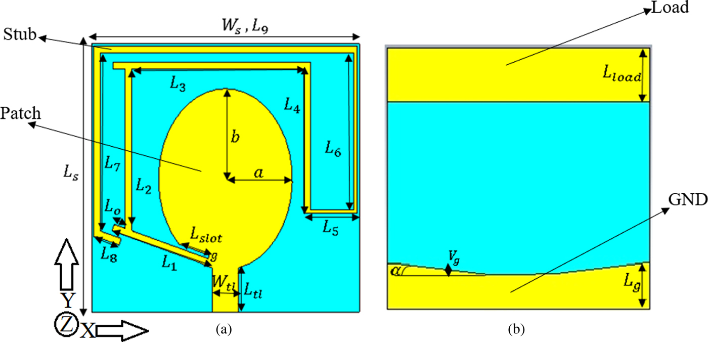
The simulated and fabricated prototypes of the proposed elliptical antenna along with the measurement setup and environment in plywood and high-density wood are presented in Figs 3 and 4, respectively. The antenna dimensions that are depicted in Fig. 3 are 20 mm × 20 mm × 1.5 mm. Furthermore, the antenna geometry illustrated in Fig. 3 is located on the X–Y plane and the designing parameters are pointed and named accordingly. In MWI, two undesired parameters that affect the reconstruction of the image negatively are the clutter and the imaging artifacts. To reduce the amount of clutter and the number of artifacts in the image reconstruction process, the number of antennas should be increased. This increase in the number of antennas enhances the scattered signals in our imaging environment. Hence, having miniaturized dimensions is helpful in terms of reducing the cost of the system. According to the authors' findings, the proposed antenna represented the lowest profile antenna applied for imaging of wood.

Fig. 3. Front (a) and the ground view (b) of the proposed antenna.

Fig. 4. Prototype of fabricated antenna and measurement in air and wood (a: high density wood, b: soft plywood, c: fabricated antenna (front and back).
After designing the antenna and investigating its key parameters, the proposed antenna is simulated, and its parameters are optimized in air with a dielectric constant of 1. Then the time domain characteristics of the antenna are investigated in high-density wood, and plywood as working environments with dielectric constant of 3 and 2.1, respectively. Both plywood and high-density wood samples are homogenous in shape and electrical properties (after testing their dielectric properties, they presented almost the same dielectric constant in each location on the sample). These types of wood are employed to show the working ability of the proposed antenna in an environment like wood. To gain an acceptable and applicable coupling between the transmitter (antenna) and wood, the antenna is simulated on polytetrafluoroethylene substrate with a dielectric constant of 2.55, thickness of 2.4 mm, and loss tangent of 0.001. The substrate utilized in the proposed antenna has a lower loss tangent than other substrates like Roggers. Since the antenna has a dielectric constant of 2.55 which is close to the wood's dielectric constant it shows better coupling.
The key parameters in the antenna designing procedure should be optimized to get the best results. These parameters can be named as patch dimensions (a, b), TL length and width (L f, W f), stub length (L 5), and the ground length. The design, simulation, and optimization process of these parameters are performed in CST software. In CST, the parameters can be optimized by defining the upper and lower limitation for each parameter. The optimization method can be chosen in this software among Genetic Algorithm (GA), Particle Swarm Optimization (PSO) and more five algorithms (GA used in our optimization due to its faster operation).
To optimize the antenna, the elliptical patch dimensions which are affecting the lower-end and higher-end of the wide BW of the antenna should be considered first. Therefore, the semi-major axis of the elliptical patch has effects on the shifting of the band to lower or higher bands (directly proportional to the wavelength) and the semi-minor axis affects the BW. In addition, the width of TL is directly related to the matching of the antenna when it is equal to the characteristic impedance of the TL.
The length optimization of the stub connected to the junction is divided into two lengths, which affect the reflection coefficient result due to their distance from the edge and the resonator. Thus, only one part is presented here, which can be named as L 5. The other parameters such as the gap (g) and the chamfer angle (α) do not affect the reflection coefficient result of the antenna dramatically, hence they are not presented in the optimization section. The antenna's dimensions achieved after optimization are presented in Table 1.
Table 1. The final dimensions of the elliptical antenna
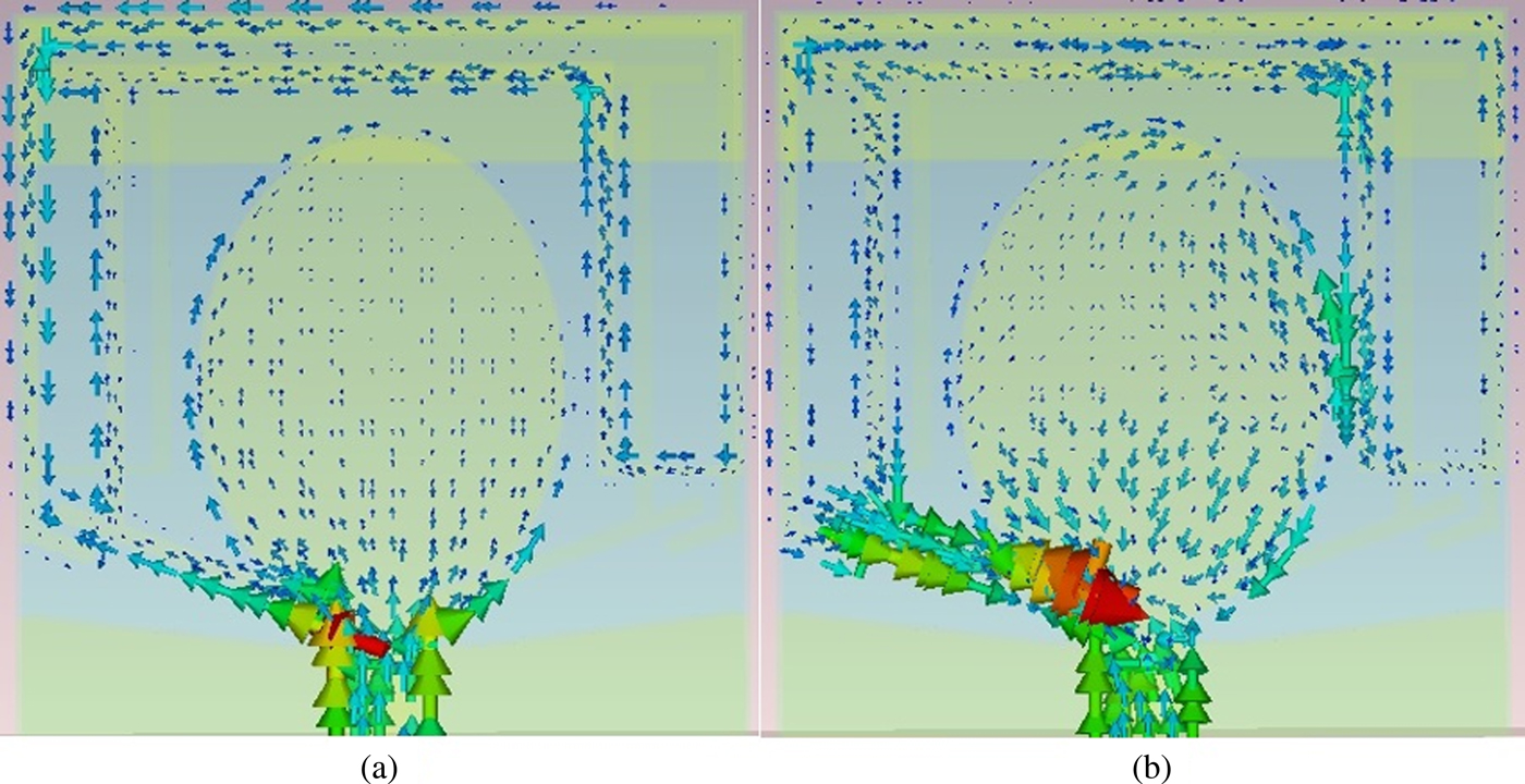
The proposed antenna has pole frequencies at 4.2, 4.8, 6.2, 8, 11.1, and 16 GHz and two resonances at lower bands at 0.9 and 1.6 GHz. Hence, the physical behavior of the guided wave to radiated wave on the proposed antenna is analyzed, representing in the simulated surface current distribution results on the radiating patch, stubs (stub connected to the patch) at frequencies of 0.9, 1.6, 2.68, and 16 GHz, as shown in Figs 5 and 6. Unlike narrowband antenna, the UWB antenna behaves in a traveling wave type that supports both fundamental mode of propagation at lower frequency and higher-order modes at higher frequencies. It is revealed that the patch, TL, and the slot on the ground are the major parts to radiate wave responding for extremely wide frequency range. On the other hand, when the current distribution paths on the patch, TL, Slot on the ground are changed or disturbed, more impact to electrical characteristics of the antenna occurs based on the quarter wave modes (Figs 5 and 6).

Fig. 5. Current distribution of antenna at 0.9 GHz (a) and 1.6 GHz (b).

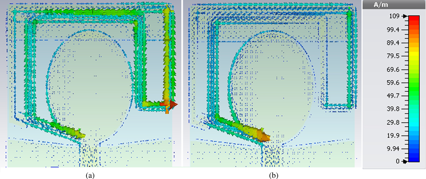
Fig. 6. Current distribution for lower-end ((a) at 2.68 GHz) and higher-end ((b) at 16 GHz) of BW.
Moreover, the surface current distributions are very strong near the edges of the stub connected to the junction at 0.9 GHz. It is obviously shown and ensured that the required length to obtain a resonance at 0.9 GHz is the same length as obtained and optimized in Fig. 5(a). The same trend goes to the current distribution as it is very strong around the edge of the slot cut from the patch near the stub at 1.6 GHz (Fig. 5(b)). Moreover, it is obviously seen that the current distribution of the antenna around the stubs, patch, and the TL as shown in Fig. 5 is more focused and has more density around the slot cut and has a resonance of 1.6 GHz [Reference Moeikham, Mahatthanajatuphat and Akkaraekthalin46]. In addition to that, the current distribution of the antenna around the lower-end and the higher-end of the antenna is demonstrated in Fig. 6. It is clearly depicted that the patch and the TL are mostly affecting the BW of the antenna and both the lower and higher end of the antenna.
Before discussing the results, it is better to show how UWB antenna operates both in time and frequency domain. Typically, narrow-band antennas and propagation are described in the frequency domain. Usually, the characteristic parameters are assumed to be constant over a few percent BW. For UWB systems, the frequency-dependent characteristics of the antennas and the frequency-dependent behavior of the channel should be considered. On the other hand, UWB systems are often realized in an impulse-based technology, and therefore the time-domain effects and properties should be known as well. For the frequency-domain description, it is assumed that the transmit antenna is excited with a continuous wave. While, for the time-domain description, it is assumed that the transmit antenna is excited with an impulse signal with the frequency f. In the frequency domain the antenna transfer functions represent a 2D vector with two orthogonal polarization components; but in the time domain, the antenna's transient response becomes more adequate for the description of impulse systems. The antenna's transient response depends on time, but also on the angles of departures and arrivals, and polarization. Figure 7 shows the procedure of sending and receiving a pulse between two UWB antennas in time domain.
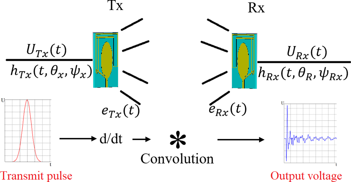
Fig. 7. UWB antenna system in time domain.
Simulated and experimental results
Input and radiation characteristics of the antenna
To do the measurement a Performance Network Analyzer (PNA) with model E8363C is used. First, the PNA is calibrated to obtain a perfect accuracy in measurement. Then, a frequency range from 500 MHz to 30 GHz and 1002 frequency steps for this range of frequency are adjusted and then the measurement in air is fulfilled. Furthermore, to measure the scattering parameters in a different medium like high-density wood and plywood, two antennas are used. One antenna is connected to terminal one of the PNA as a transmitter (Tx) and the other one is connected to the second one as receiver (Rx). The Tx is fixed at the center of the wood and the other antenna touches the other side of the wood slice according to the array's locations as shown in Figs 13 and 5. In each step, the Tx is fixed, and the Rx is located on array locations. Afterward, the scattering parameters (the reflection and transmission coefficient) for each array are extracted from PNA and imported to MATLAB to be evaluated for time domain considerations.
Based on both the simulation and measurement results shown in Fig. 8, the proposed antenna has an acceptable reflection coefficient and working BW. Figure 8 illustrates that the proposed antenna can be assumed as a UWB antenna since it obtains more than 13.25 GHz BW at center frequency of 10 GHz of the entire frequency band. Besides, the measurement and simulation results are in good agreement.
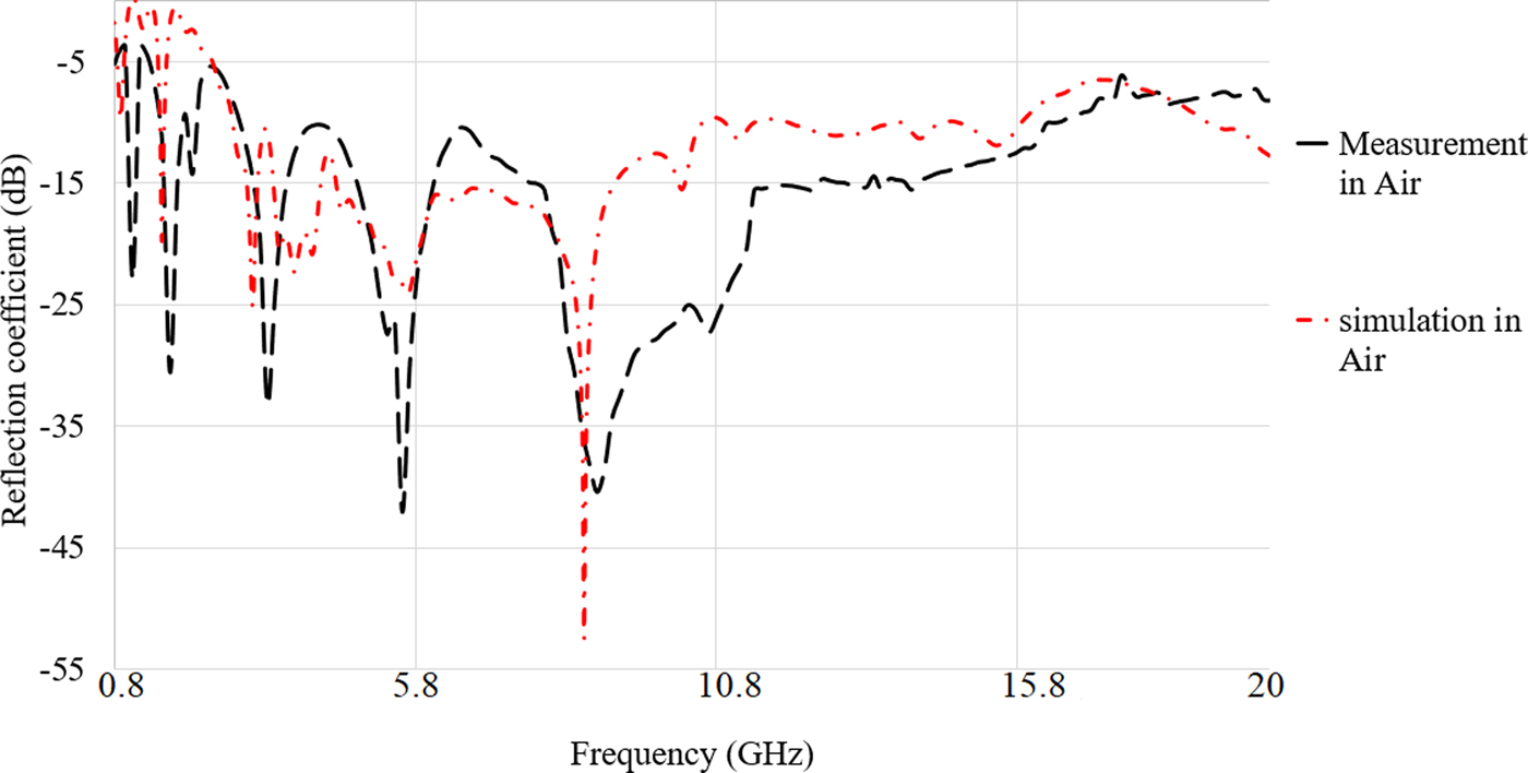
Fig. 8. Measured and simulated reflection coefficient result of proposed antenna in air.
It is clearly shown in Fig. 8 that the resonant frequencies at both 0.9 and 1.6 GHz are achieved with only a slight shift, but the antenna is still working, and they are within the BW. Furthermore, most of the working frequency band are obtained (2.68–16 GHz) and it is just shifted slightly from 2.68 GHz in the simulation result positively. Apart from that, the stop- band after 16.2 GHz is removed in the measurement result and the reflection coefficient level is better than simulation, which is acceptable (VSWR < 2). In addition, the optimum required BW for imaging of wood is obtained. The proposed antenna's BW is enhanced to have the antenna working at higher bands, which is useful for other applications like skin cancer, which needs low penetration (previous studies applied even a low THz for skin cancer).
The first difference between the simulation and the measurement results in the reflection coefficient is due to the differences that occurred after fabrication. The next one is due to the simulated conditions and the measurement conditions are not the same, and tolerances during the fabrication process may affect the results after fabrication.
In addition to that, in CST the waveguide port is usually used for feeding the antenna from the macros section, as the software does it automatically after calculating the port dimension based on microstrip line equations and substrate thickness and width of the feedline. At upper-frequency range, the exposed center pin of the SMA port causes significant radiation, so reducing the length of the center pin limits the unwanted radiation from the connector. The simulation result in [Reference Xu, Wang, Wang and Wu47] showed that the shorter the center pin, the smaller VSWR is. To ease the soldering and the reliability of the connection, the center pin is chosen to be 0.5 mm. Besides, soldering should be done carefully not to increase the resistivity of the ground using too much tin in soldering.
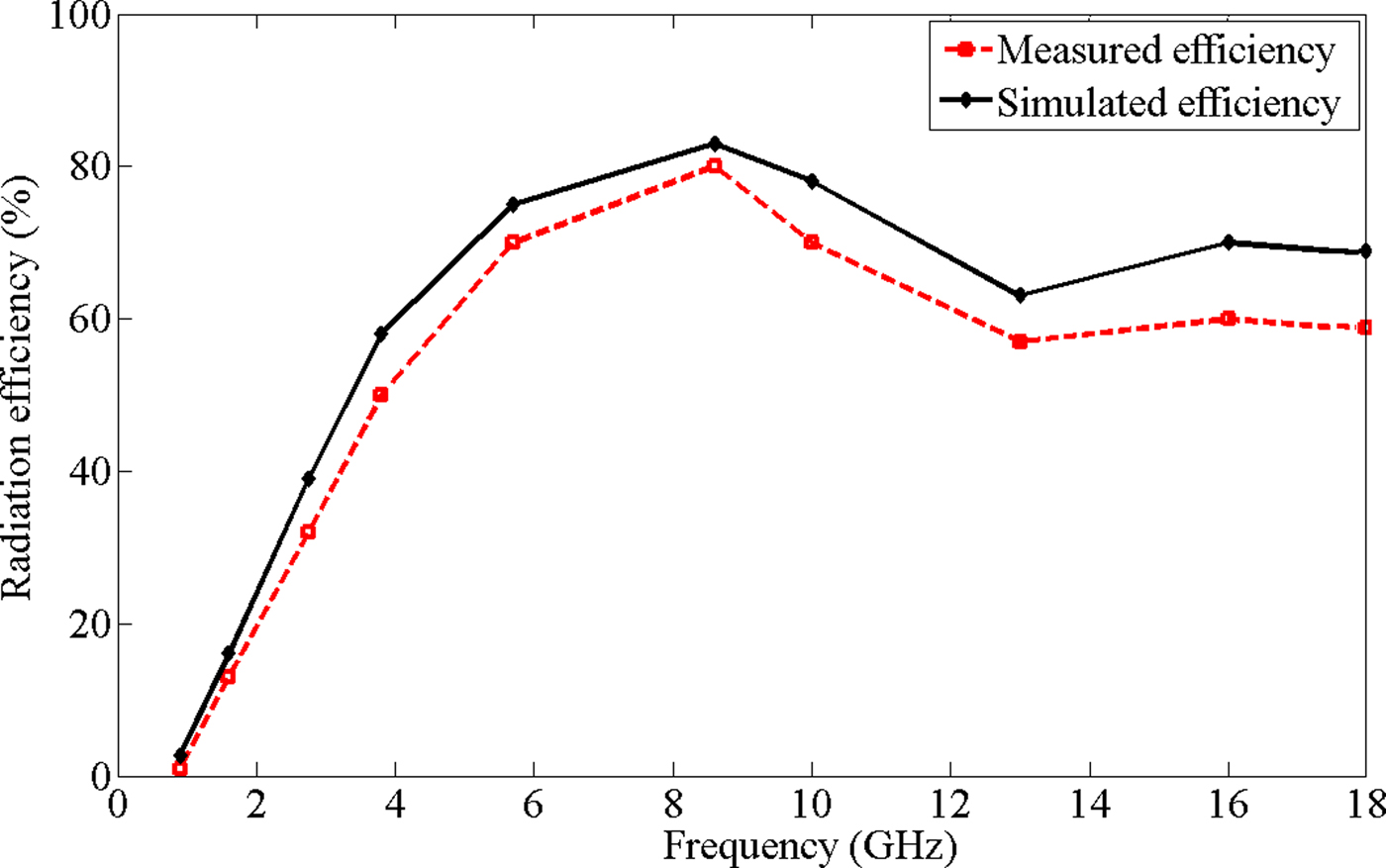
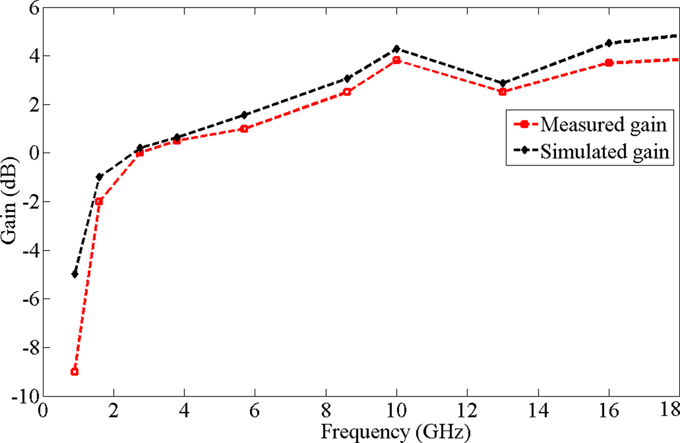
Figures 9–11 present the simulated and measured antenna's far-field radiation pattern for both E and H planes at each pole of the antenna, gain, and radiation efficiency. The far-field radiation pattern of the antenna is shown in this paper to investigate how an antenna works if it is considered for applications that need far-field. After the simulation radiation patterns are performed, radiation patterns at some select frequencies for each antenna are measured. The radiation patterns are measured using a SATIMO Starlab near-field measurement system. While each antenna works over a large frequency range, the patterns are measured at each pole and the lower and higher-end of the ultra-wide BW to show the overall behavior at the low, mid, and high-frequency ranges. Based on the measured results, the gain increases with the operational frequency of the antenna as attained from the simulated results. In addition, the beamwidth decreases as the frequency increases, which contributes to the increased gain. The radiation pattern shows a slight deviation of ±(1–3) dB for several reasons. In the system, the angles which catch the maximum pattern and gain are difficult to obtain based on the placement of the antenna. Secondly, the sensitivity of the connector placement for the coaxial feed can have a large impact of the measured results. The surface roughness of the copper may also have an impact on the results. The discrepancy between the measured and simulated results of the antennas becomes more apparent in the higher frequency patterns. Also, the silver paste used to fix the antenna and the coaxial cable together has a larger loss at higher frequencies. Overall, the measured patterns match relatively well with the simulated results, showing the potential of 3D printed antennas for use in UWB antenna applications.
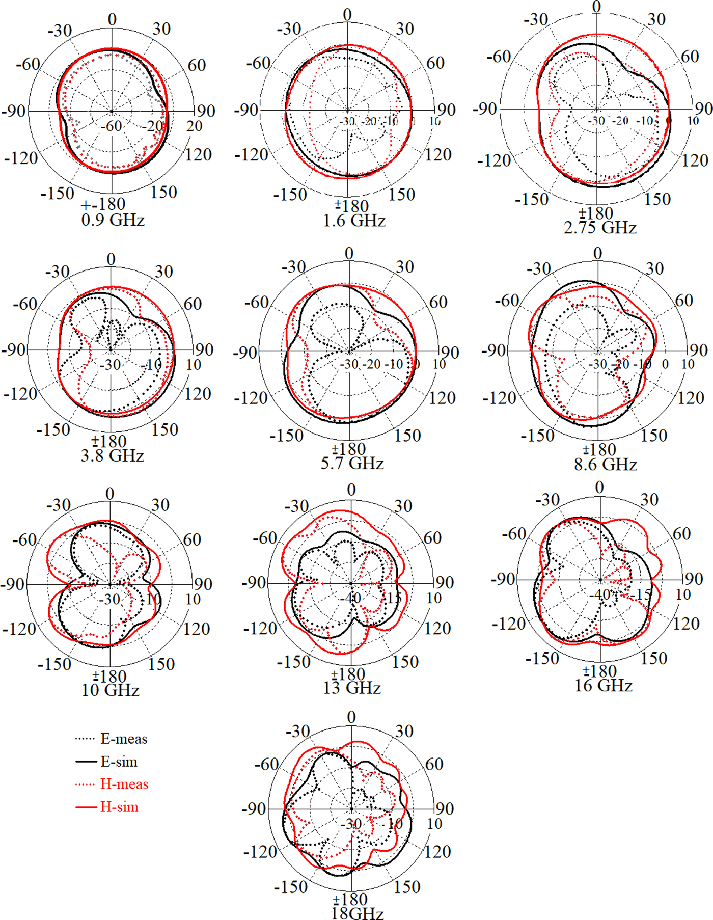
Fig. 9. Simulated and measured radiation pattern in both E and H planes at 0.9–20 GHz.

Fig. 10. Simulated and measured radiation efficiency.

Fig. 11. Simulated and measured radiation gain.
Sensitivity of the antenna performance to fabrication tolerances
Since the antenna structure is complex and it consists of stubs and slots, it would be informative if the sensitivity of the antenna performance to fabrication tolerances is provided (Fig. 12).
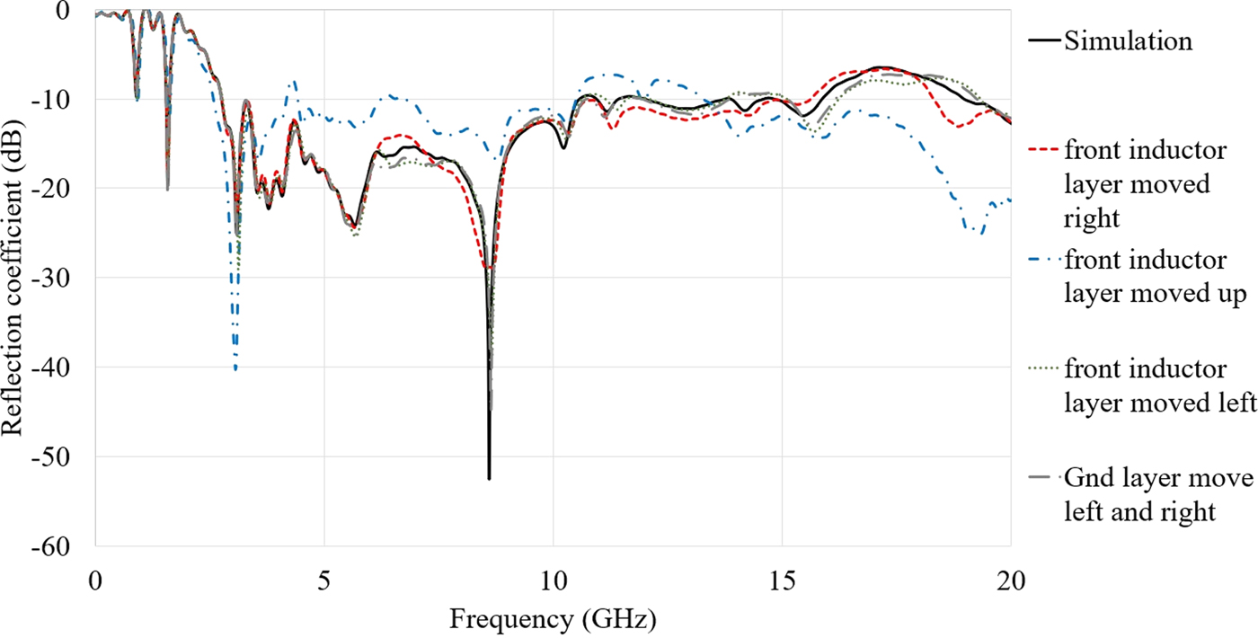
Fig. 12. Reflection coefficient result of the antenna for sensitivity to fabrication tolerance (gnd is the Ground layer, ver means vertical, hor is horizontal, and pat is the patch).
For example, the antenna's performance is clear when the layers are perfectly aligned (without tolerance) as compared to when there is a horizontal (“hor” in Fig. 12) or vertical (“ver” in Fig. 12) misalignment of the layers (the misalignment might be caused by fabrication). Figure 12 clearly shows that when there is tolerance in fabrication of the antenna, the reflection coefficient results of the antenna change according to the amount of misalignment. This tolerance makes some stop bands in the working BW so as more resonances in the lower band.
The design, simulation, and optimization process of these parameters are performed in CST software. The solver used in CST to calculate the time domain considerations section is Time domain solver which uses the Finite Integration Technique applies some highly advanced numerical techniques such as the Perfect Boundary Approximation® in combination with the Thin Sheet Technique™ to allow accurate modeling of small and curved structures without the need for an extreme refinement of the mesh at these locations. This allows a very fast memory-efficient computation along with a robust hexahedral meshing to successfully simulate extremely complex structures. Furthermore, in CST, the parameters can be optimized by defining the upper and lower limitation for each parameter. The optimization method can be chosen in this software among GA, PSO and more five algorithms (GA used in our optimization due to better results).
Time domain considerations
Transmission response
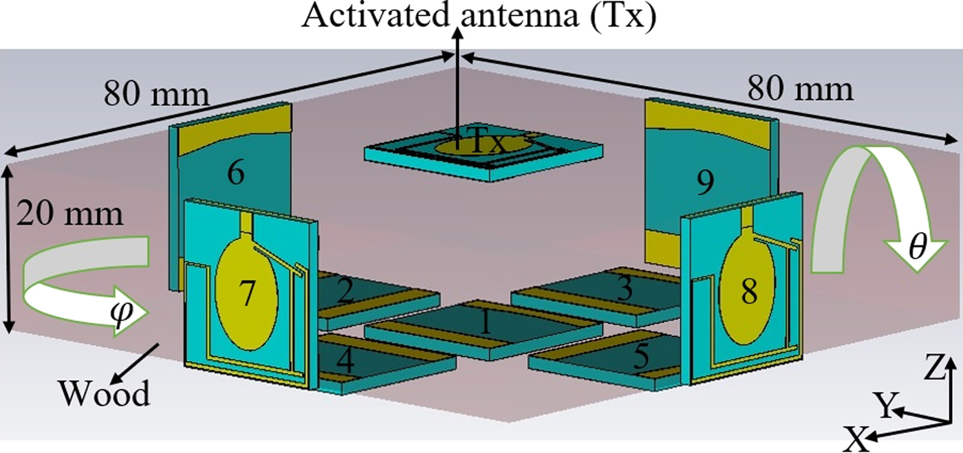
The measurement setup is presented in Fig. 13. The wood slab dimensions are 45 mm × 45 mm × 20 mm. The antenna positions and the angles at which they are located during the measurement are depicted in Fig. 13. The same method as is done in simulation to obtain the time domain characteristics of the array antenna is performed in measurement. In measurement, Tx is kept fixed and then the array antennas A1–A9 are located at the location base as shown in Fig. 13. Afterward, the time domain characteristics are investigated for each array.
To have the lowest possible distortion in the signal transmitted from the proposed antenna to the sample, the transmission response (S 21) needs to be flat at the desired working frequency BW [Reference Lamensdorf and Susman48, Reference Hraga, See, Abd-Alhameed, Jones, Child, Elfergani and Excell49]. In addition, the reflection coefficient result (S 11) should present an acceptable result and should not vary too much from the simulated result in air. Since S 11 shows how much of the wave is reflected when the wave is passing through an environment other than air, it should be <−10 dB to be acceptable.

Fig. 13. Simulation setup (it has been followed by measurement setup and arrays 1–4 are moved based on the θ and the arrays 5–9 based on φ).
Based on both simulation and measurement results as shown in Fig. 14, the proposed antenna shows an acceptable reflection coefficient and working BW at 0.9, 1.6, and 2.68 GHz to up to 16 GHz. The first two low frequencies at 0.9 and 1.6 GHz make the antenna capable of working in ISM and L-band. Despite narrow BW at these two bands, they can be helpful in imaging purposes at low frequencies for more penetration. Besides, Fig. 14 illustrates that the proposed antenna can be assumed as a UWB antenna since it was able to obtain more than 13 GHz BW at a center frequency of 10 GHz. Besides, the measurement and simulation results show good agreement. It is clearly shown in Fig. 14 that both resonance frequency at 0.9 and 1.6 GHz are achieved with only a slight shift, but the antenna is still working, and they are inside the BW. Furthermore, most of the working frequency band are obtained (3.3–13.3 GHz) and it has just a bit shifted from 2.68 GHz in simulation result. In addition, the optimum required BW for both imaging in wood and medical purposes (until 10.6 GHz) is attained. The proposed antenna's BW is enhanced to have an antenna working at higher bands which is useful for other medical application like skin cancer and needed low penetration (previous studies applied even low THz for this purpose). The measurement result of the antenna for different environments than air is depicted in Fig. 14. The first two resonances are degraded for high-density wood while in BW they have better level of reflection coefficient for plywood. Besides, it shows that for most of the BW the antenna worked for plywood except for some stop-bands that occurred from 4.5 to 6.5 GHz. High-density wood due to its physical properties and higher dielectric constant cannot pass the signal as compared with the plywood. The differences occurred between the simulated and measured results are due to: first, the differences occurred after fabrication. The next one is the simulated conditions and the measurement conditions are not the same and tolerances during the fabrication process may affect the results after the fabrication.

Fig. 14. Measured and simulated reflection coefficient result of proposed antenna in air and wood.
To minimize the distortion in the transmitted signal through the wood, it is required that the S21 is as flat as possible in the required frequency BW [Reference Ahadi, Binti, Isa, Bin Saripan, Zuha and Hasan23]. Figure 15 depicts the measured transmission response of the proposed antenna based on the measurement setup in Fig. 13. To perform the measurement of transmission coefficient, two antennas are located at both side of the wood sample (plywood and high-density wood) with thickness of 20 mm and in air with the distance of 20 mm. The simulated S21 in Fig. 15 shows almost 5 dB variation in the frequency range of 3–12 GHz while this level is reduced at higher frequencies. The S21 variation is decreased by almost 10 dB for measurement in air. The same trend goes with the measurement of plywood and high-density wood at frequency range of 3–12 GHz. After 12 GHz the transmitted power is dissipated within the wood because of the lossy material (higher relative permittivity). Moreover, when the frequency is higher than 12.5 GHz, the transmission response is degraded by more than 10 dB. This reduction in S 21 and distortion are due to the decreasing of the wavelength at higher frequency, and due to the higher dielectric constant of high-density wood and plywood compared with air. Since the substrate chosen for this antenna had a dielectric constant (2.55) near to both high-density wood and plywood, their results did not differ greatly.
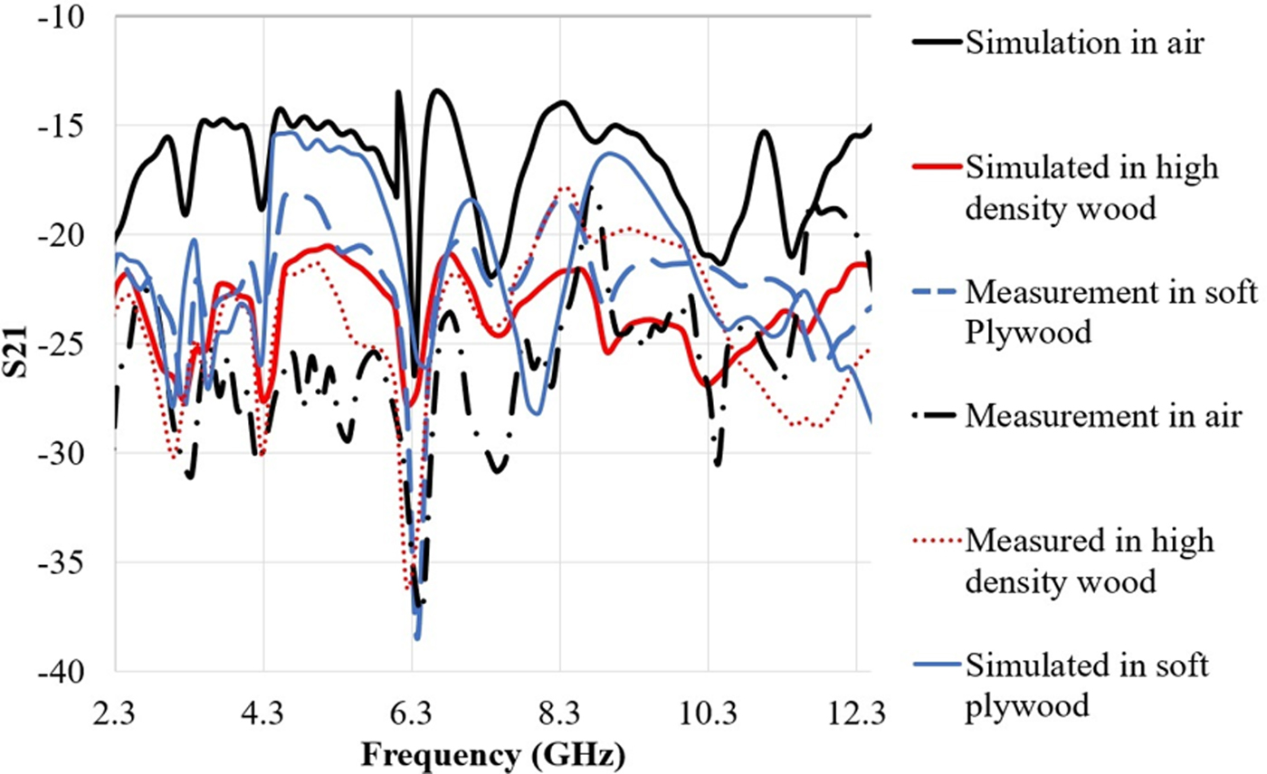
Fig. 15. Simulated and measured transmission response S 21 in different environment.
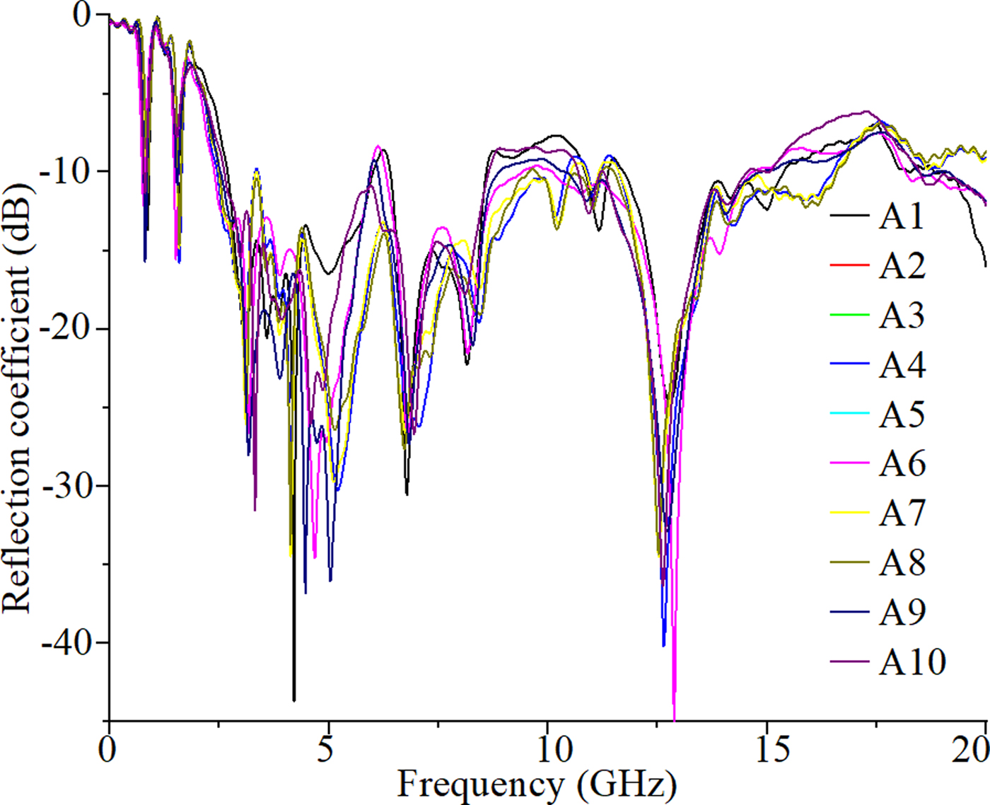
The amplitude reflection coefficient results for each of the antenna array at the presence of the other array antennas are presented in Fig. 16. As indicated in Fig. 16, the reflection coefficient has a higher level at some frequencies between 5.5 and –7 GHz, 10–11 GHz, and 17–18 GHz. This change in the reflection coefficient indicates the loading effects due to the presence of other antennas. It can also give an indication as to which working frequencies should be selected for the MWT operation.

Fig. 16. Reflection coefficient amplitude of each antenna in the presence of other antennas.
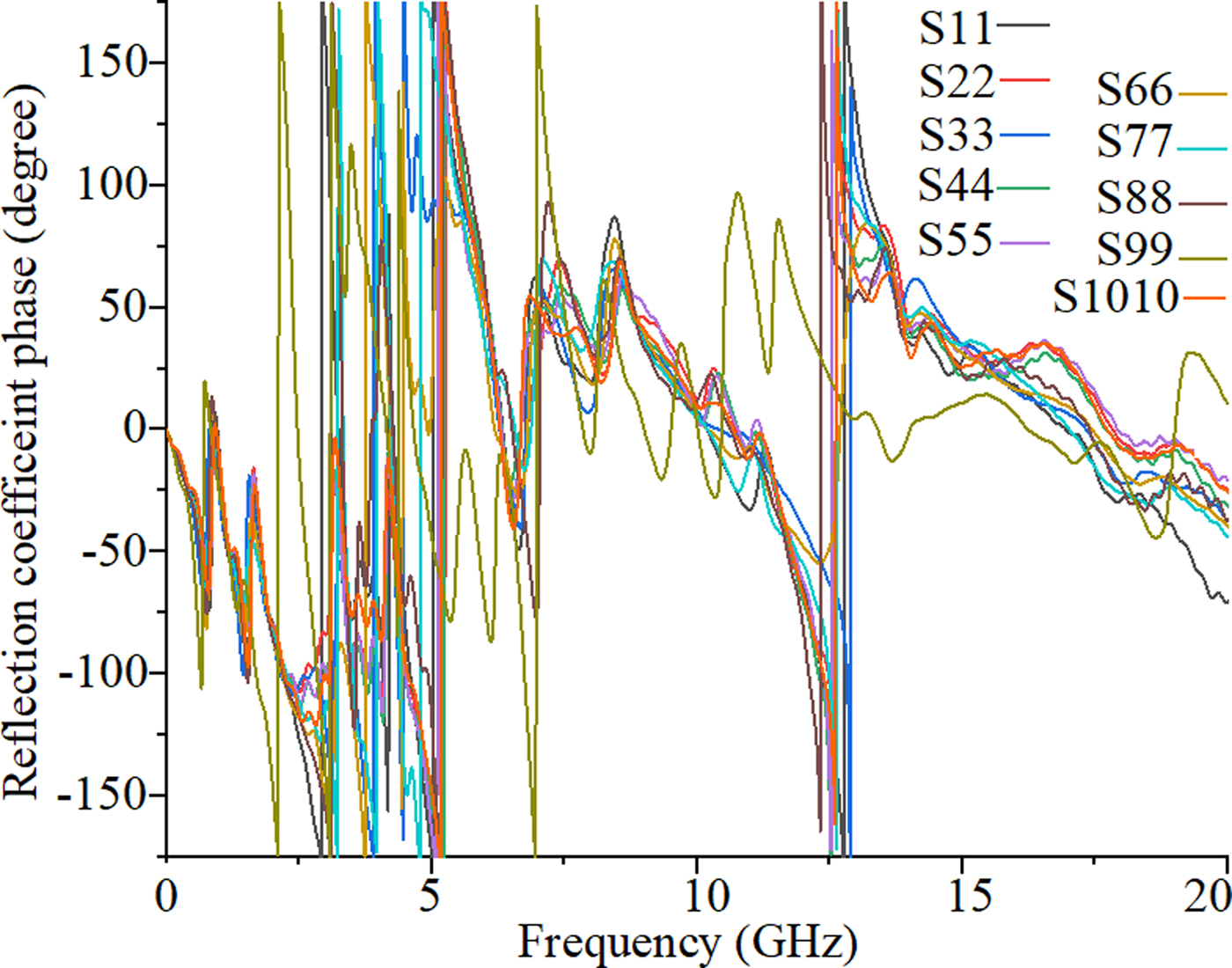
Besides, the image reconstruction error is lower at frequencies where the reflection coefficient is invariant. Figure 17 shows the reflection coefficient phase of the proposed antenna when it is alone and when nine arrays are located around it in both X and Y-directions. It is clearly illustrated that when the antenna is located among the arrays, the reflection coefficient phase of the antenna slightly changes due to the loading effects of the other arrays on each other.

Fig. 17. Reflection coefficient amplitude result of antenna alone and at the presence of nine arrays (A1–A9).
Furthermore, it shows linear phase variations except for A9 which is farther than Tx main lobe and its reflection coefficient is so affected by the loading effects of A3, A6, and A8.
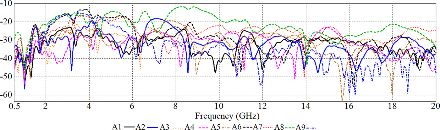
Figure 18 shows the transmission coefficient results between the antenna (Tx) and other antennas, which highlights the level of mutual coupling and isolation. As shown in Fig. 18, the mutual coupling is <−20 dB at most of the band except coupling with antenna 1 which is <−13 dB at frequencies 7.8–9 GHz and there is a good isolation between elements at these frequencies. Transmission coefficient amplitude and phase evaluation are used to identify the level of mutual coupling. Figures 18 and 19 present good isolation at most of the frequency band since the transmission coefficient amplitude is <−20 dB at most of the BW. Although, at some frequencies it is near to −20 dB, it increases to almost −15 dB at 3–4 GHz and 5–6 GHz. When one antenna is located at the front of the proposed antenna at Phi = 0, frequencies from 3 to 4 GHz and 7.8–9 GHz showed higher transmission coefficient near – 15 dB and −13 dB thus at these frequencies higher mutual coupling and lower isolation occurred in comparison with the other frequencies. Furthermore, not too much variation in phase is noticed in Fig. 19 and the phase variation is linear except the phase variation at theta = 90° changes because of the antenna loading effects of the other arrays around it.

Fig. 18. Amplitude of mutual couplings between antennas.
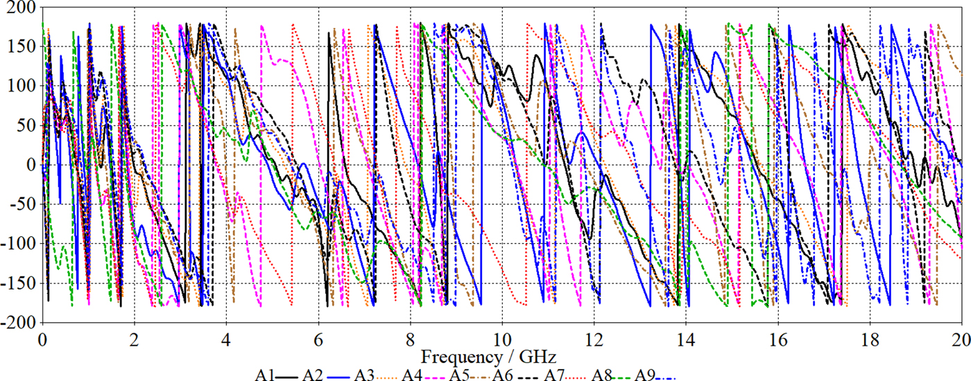
Fig. 19. Transmission coefficient (S 21) phase of the antenna with the arrays around it (a: in phi direction, b: in theta direction).
Figures 20–22 indicate the transmitted and received signals, respectively.

Fig. 20. Transmitted pulse from the transmitter antenna.
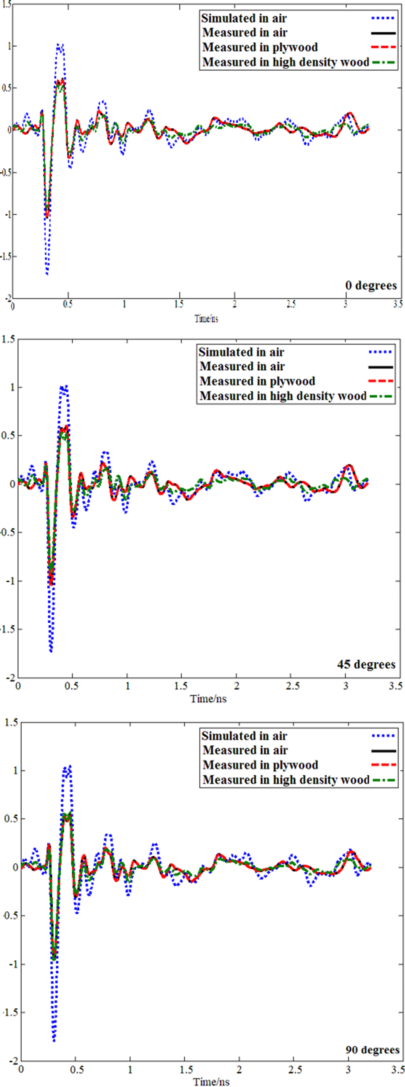
Fig. 21. Received signals for simulated and measured in soft plywood, air, and high-density wood (φ = 0–90°).

Fig. 22. Received signals for simulated and measured in soft plywood, air and high-density wood (φ = 135° − 90°).
In Fig. 20 h(t) is the time domain impulse response and |h^ + (t)| is the envelope of the impulse response which localizes the distribution of energy versus time and it can be a direct measure for the dispersion of an antenna. The peak value p (θ,ψ) of the envelope shows the strongest peak of the antennas time domain transient response envelope. The envelope width (τ) demonstrates the broadening of the radiated impulse and is determined as the magnitude of analytic envelope at half maximum. It should not exceed a few hundred picoseconds to obtain the high data rate and high resolution in communications. Furthermore, the ringing of a UWB antenna is an undesired parameter and is normally caused by resonances due to energy storage or multiple reflections.
Besides, ringing is defined as the time until the envelope has fallen from the peak value to a certain lower bound and it should be negligibly small less than a few envelop width. The energy or the ringing is not used at all and it can be eliminated by e.g., absorbing materials. Based on the measurement setup presented in Fig. 13, antenna Tx keeps fixed and antenna A1–A9 are moved around the antenna Tx at different angles (first two antennas are located at boresight direction then is moved to the other angles). Antenna Tx transmits the signal depicted in Fig. 20 and then the other antennas receive the signal presented in Figs 21 and 22 at different angles from 0° to 180°. The simulated received signals in air show the highest amplitude. When the environment changes to high-density wood and plywood, due to the higher dielectric constant, the amplitude of the received signals is changed and decreased. The plywood received signals show better results than high-density wood due to the lower dielectric constant compared with the high-density wood. Besides, the total shape of the signal when transmitted from antenna Tx and after passing through the environment with different dielectric constants is not changed (Figs 21 and 22 show the received signals in different angles (φ) from 0° to 180°. It is obvious that the signals' shape did not change dramatically except the signal's amplitude. Besides, the signal's similarities and low distortion in signals are proven with fidelity percentage later in Fig. 23). Hence, the proposed antenna can be an acceptable device to act as a send/receive device in a medium such as wood. In simulated and measured results of the time domain considerations, for each MW frequency, a resonant effect might occur that register in receiving antenna as an amplification of the signal. This explains why some materials like plywood can express higher transmission. In addition, plywood has less dielectric constant compared with the high-density wood. Thus, the transmitted signal can be penetrated more into the material.
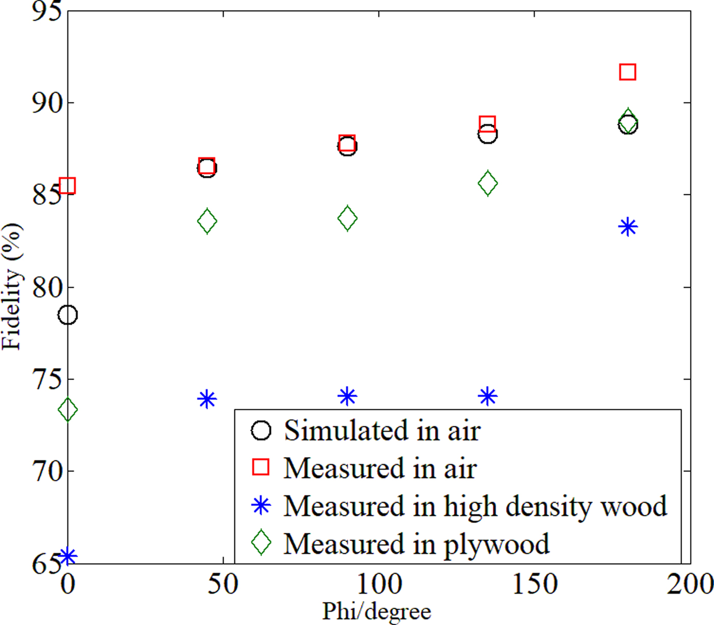
Fig. 23. Fidelity of the proposed antenna (%) in different degrees and environment.
To achieve the received signals in Figs 22 and 23, first the transmission response in a different angle of Phi, 20 mm distance (Thickness) and different environments, should be extracted from PNA (model E8363C). Then the Fast Fourier Transform (FFT) of the transmitted pulse is calculated to get the frequency response. Afterward, the transmission response is multiplied with the frequency response of the pulse to obtain the received signal in the frequency domain. Besides, to get it in time domain an inverse FFT (IFFT) is required [Reference Ahadi, Binti, Isa, Bin Saripan, Zuha and Hasan23].
Fidelity factor
It is required to calculate the signal fidelity since the distortion in the signal is a critical issue. In addition, fidelity can be considered as a magnitude of the cross-correlation when it reaches its maximum between both the transmitted and received pulse. After achieving the received signals in the time domain from the last section, the fidelity, F, can be obtained as follows [Reference Montoya and Smith50]:
 $$F = {{\mathop \int \nolimits_{-\infty} ^{ + \infty} x(t)y(t-\tau )dt} \over {\sqrt {\mathop \int \nolimits_{-\infty} ^{ + \infty} \vert {x{(t)}^2} \vert dt\; \mathop \int \nolimits_{-\infty} ^{ + \infty} \vert {y{(t)}^2} \vert dt}}}, $$
where x(t) is the transmitted pulse from one antenna, y(t) is the received pulse in another antenna, and τ is the shift or delay the signal received by the second antenna.
The antenna's fidelity with 20 mm thickness of wood and in different angles is depicted in Fig. 23. Due to high fidelity presented in Fig. 23, low distortion is obtained in the transmitted signal since it is more than 65% and the proposed antenna can be recommended for using MWI of sample like wood [Reference Islam, Islam, Rashed, Faruque, Samsuzzaman, Misran and Arshad51]. In addition, Fig. 23 illustrates a high percentage of fidelity in all the three environments. It is obvious that the fidelity percentage is the highest for the measured result in air and it is followed by the result for simulation and plywood. Furthermore, the lowest percentage belongs to the high-density wood.
Group delay
When the distortion in the signal phase becomes a critical issue, a factor like Group Delay (GD) should be considered well. Figure 24 illustrates the proposed antenna's GD for various distances (5–100 mm) between transmitter (antenna1) and receiver (antenna 2). It demonstrates that when the distance increases, the GD increases as well. The increment is because of the heterogeneity in various environment and frequencies. Since GD has a direct effect on widening the resolution cell, the antenna should be designed in a way to keep the instantaneous error less than one resolution cell. The FFT should be 1/T as well. Moreover, the maximum GD can be calculated as follows:
 $$D_t \lt 1/f_s.$$
Fig. 24. Simulated group delay in different thickness of wood.
In the above equation f s is the low resonance frequency [Reference Ahadi, Binti, Isa, Bin Saripan, Zuha and Hasan23]. In medium with high thickness, the lowest resonance frequency should be reduced. For the current work the lowest resonance is 0.9 GHz, therefore the maximum GD becomes 5.5 ns.
Near-field radiation intensity
The near-field characteristic of an antenna is an important parameter in MWI. The proposed antenna's near-field intensity pattern drawn at 5 cm distance from the antenna at XZ-plane is shown in Fig. 25. It is clearly presented in Fig. 25 that the antenna radiated most of its power to the wood. Hence, it can be a good device for MWI in wood. For acquiring the near-field pattern in CST, 360 probes are put in 5 cm distance around the antenna for both E-field and H-field. Then these fields in each direction (X, Y, Z) are extracted from CST. Afterward, the data are imported to MATLAB to calculate and draw the near-field radiation intensity pattern of the antenna.
Fig. 25. Near-field radiation intensity of the antenna.
The proposed UWB antenna is compared with recent similar existing antennas for imaging purpose and is shown in Table 2. In addition, the antenna's performance is checked in terms of some parameters such as applications, 10-dB BW, dimensions, directivity, and gain. However, the proposed antenna may not have higher gain than some works presented in [Reference Ahadi, Binti, Isa, Bin Saripan, Zuha and Hasan23,60], but a good fractional BW (FBW, >133.3%) is achieved. Since the proposed UWB antenna is in low profile, more antenna can be exploited for MWI of wood. In addition, high performance can be achieved while the antenna dimensions are maintained small compared with the recent works presented in [Reference Eesuola, Chen and Tian13,Reference Bourqui, Campbell, Williams and Fear52–Reference Gupta, Khound, Surana, Susila and Rao59,Reference Elahi, O'Loughlin, Lavoie, Glavin, Jones, Fear and O'Halloran61,Reference Mirbeik, Li, Garay, Nguyen, Wang and Tavassolian62].
Table 2. Comparison of the proposed design with previous similar works

Imaging of the sample
Data for the UWB MWI techniques are acquired from array antennas around the samples (Fig. 26). Each element in the antenna array sequentially transmits a UWB pulse into the wood sample and then the backscattered signals are recorded for the illustration of the feasibility of the applied DAS algorithm in detecting even the small defects. A total of M × M (number of arrays) backscattered signals are recorded after all the elements have taken their turn to transmit.

Fig. 26. Image reconstruction setup.
The recorded backscattered signals include early-time and late-time contents. The early-time content is dominated by the incident UWB pulse, reflections from the wood, and residual antenna reverberations whereas the late-time content contain defect (hollow) response. The goals of signal processing are to reduce the early-time content, which is of much greater amplitude than the defects response, to suppress the clutter in the late-time content with minimum distortion level to the defect's response, and to enhance these desired responses so that reliable defects detection in the reconstructed image can be achieved.
Furthermore, the next step after simulating, the device in CST analyzes the scattered pulses exported from CST. The presented formula for signal analyzing is coded in MATLAB. This code receives time domain output from CST and converts the scattered pulses into an image. The MATLAB code gets the scattered pulses from CST, calculate the distance of a focal point to the antennas, calculate the delays, remove the delay from the pulses, sum all the pulses, and calculate the intensity of the pules for that focal point. These steps are repeated for all the focal points in the wood. The results for each focal point are recorded in a 3D matrix. At the end of the analysis when all the focal points are considered, the data recorded in the matrix will be used as an image which can be used to show 2D or 3D images from inside the wood.
The first step in processing the scattered pulses is to calculate the time delay for a focal point. This can be done by a MATLAB code by considering the antenna numbers in it. This code calculates the delay which starts with the first antenna and calculates its distance to the focal point as d 1. The next loop starts from the next antenna until the final antenna to calculate d 2. After calculating both distances, the delays will be calculated. Afterward, the delay is removed from the scattered pulses for that focal point. Then, a loop is used to add all the scattered pulses after delay cancelation. When the summation finishes, the intensity of the scattering pulses will be used as the result for that focal point. All the steps should be repeated for all the focal points [Reference Elahi, O'Loughlin, Lavoie, Glavin, Jones, Fear and O'Halloran61].
In addition to that, another factor for imaging is to define the axial resolution which is defined as the minimum detectable feature size in the direction of wave transmission, limited by the BW of the system and is given in [Reference Mirbeik, Li, Garay, Nguyen, Wang and Tavassolian62]. Furthermore, to show the capability of the antenna in reconstructing image, a sphere with a radius of 2.5 mm is located at center of the wood sample as shown in Fig. 26. To reconstruct the image, the Delay and Sum (DAS) algorithm are used to show the image of the sphere within the wood sample.
Figure 27 illustrates the reconstructed image using DAS algorithm. It clearly shows that the antenna can be an adequate candidate to detect a hollow in wood. However, the exact and complete shape of the hollow (sphere) in wood sample could not be detected. The accuracy of the image can be improved by applying another algorithm mentioned before like DMAS.
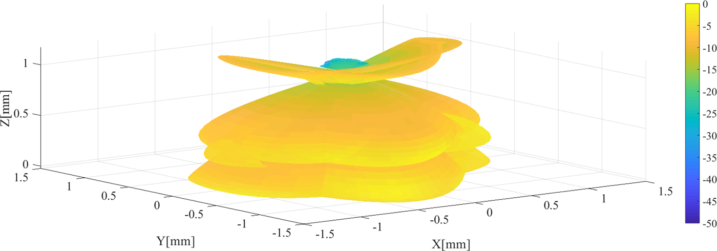
Fig. 27. 3D image of the hollow in wood sample showed in Fig. 26.
Conclusion
A UWB antenna with miniaturized size is presented for MWI in wood. The proposed UWB elliptical microstrip antenna is designed to radiate in the wood environment. The proposed antenna comprises an elliptical patch, fed by a TL, a stub connected to the junction between the patch and TL, and a slot cut from the patch use to have two more resonances at 0.9 and 1.6 GHz. It shows an acceptable feed match at 2.68–16 GHz frequency band, 178° 3 dB beam-width in φ = 0° and 165° in φ = 90° plane, respectively. In addition, the maximum gain of 5.48 dB and directivity of 6.9 dBi is achieved. Both the simulated and measured results for transmitted and received signals show low distortion through three types of wood and air. Since the antenna's transmission response (S 21) is almost 5 dB at most of the frequency band (2.68–16 GHz), the UWB antenna is suitable for imaging in wood especially when both the simulated and measured received signals show a good agreement and the measured signals' shape is not changed in different environments. In addition, the proposed antenna shows high fidelity in both received and transmitted signals in various mediums. In accordance with the achieved results, the proposed antenna seems to work adequately for MWI of wood.
Author ORCIDs
Tale Saeidi, 0000-0002-0995-3364.
 Tale Saeidi was born in Mashhad, Iran in 1985. He received his Bachelor of Science degree in Telecommunication and Electrical Engineering from Khayam University of Mashhad in 2009 and he completed his Masters in wireless Communication Engineering from Universiti Putra Malaysia in 2015. Currently, he is working as a graduate assistant in Universiti Teknologi Petronas, Malaysia. His research interest includes dielectric measurement of MW absorber materials, microstrip antenna design for MW, mm-wave and THz frequency bands. Furthermore, metamaterial array antennas in MW and UWB imaging.
 Dr. Idris Ismail is an Associate Professor at Universiti Teknologi Petronas. He is currently working as a lecturer under the Electrical and Electronics Engineering Department. Currently, he is also a member of SKG14-LT (Petronas Instrument Skill Group 14 -–- Leadership Team). His research topics include IoT and Data Analytics, Plant Process Control, Electrical & Instrumentations, and Electrical Process Tomography. Previously he had worked 11 years in Petronas Operating Unit such as refinery and petrochemical complex at Petronas Penapisan Terengganu and Ethylene/Polyethylene. He worked as I/E Engineer in Project and Maintainance until he became Head of Instrumentation at Ethylene/Polyethylene. He is also a registered Professional Electrical Engineer with Certified Practice.
 Wong Peng Wen graduated from University of Leeds in 2005 with BEng (1st Class Hons.) degree in Electrical & Electronic Engineering. He received Switched Reluctance Drive Award in EE Engineering. He did his Ph.D. study at University of Leeds, the UK from 2007 to 2009. During his Ph.D., he was involved in the UK DTI funded project, developing process design kits for multilayer system-in-package modules. Currently, he works as Associate Professor in Universiti Teknologi Petronas and received outstanding researcher award in 2013, publication award in 2014, and Potential Academy Award of the Year in 2015. His research interests include reconfigurable filter, lossy filter design, and passive filter miniaturization techniques. He has secured various research grants since 2008 and has published more than 60 papers. He is currently the chair of IEEE ED/MTT/SSC Penang Chapter, founder and organizing chair of IEEE International Microwave, Electron Devices and Solid-State Symposium IMESS 2016.
 Adam R. H. Alhawari was born in Jordan. He received the Ph.D. degree in Wireless Communications Engineering from Universiti Putra Malaysia, Malaysia in 2012. Currently, he is an Assistant Professor at the Department of Electrical Engineering, College of Engineering, Najran University, Saudi Arabia. His main research interests are in metamaterials, development of UWB antennas, microwave absorbers, and RFID.
Appendix
Antenna optimization
In the optimization process of the proposed elliptical patch antenna, the most effective parameters on the impedance bandwidth of the antenna such as the patch dimensions, TL dimensions, L 1 and L g are optimized after their actual values are obtained from the microstrip patch antenna and TL equations. The other parameters such as chamfer angle of the ground (α), the gap slot cut from the patch (g), length of the loaded stub (L 1 − L 9), length of the loaded strip at the back (L load), and width of the cut rectangular at the back (V g) are not investigated here. Increasing and decreasing of substrate dimensions shift the frequency to higher or lower band of frequency due to their direct relation with the wavelength. Figure 28 shows the optimized dimensions of the TL. It demonstrates that when the width of the patch has a maximum value of 1.5 mm, the antenna has a good impedance BW. In addition, increase in the length of the TL shifts the total BW to the lower frequency bands. But, this increment produces stop-band around 6 and 12 GHz. This change in the working BW is due to the enhancement of the distance between the patch-TL junction and the ground at the back.
Fig. 28. The transmission line dimensions (L, W).
Figure 29 illustrates that increase in patch dimensions (a and b) shifts the working band to the lower band along with widening the BW in both the higher-end and lower-end of the band. However, this act produces one stop-band around 10 GHz. Besides, when the patch dimensions are small, no stop-band occur, but the band shifts to the higher band of frequency. Furthermore, both TL and the patch dimensions have direct effects on making the lower-end and higher-end of the ultra-wide BW (the current distribution and its concentration around the patch and TL at the related frequencies were illustrated before).
Fig. 29. The patch dimensions (b, a).
The L 5's reflection coefficient variation is presented in Fig. 30. It is quite clear that by increasing this part of the stub, the resonance frequencies shift to the higher frequency band. However, the frequency band from 2.8 to 16 GHz are shifted too much but the reflection coefficient level decreased for most of the band and more stop-bands occurred. When the length is 1.8 mm the antenna does not work well in terms of the impedance BW matching as well as the length more than 4 mm. The surface waves dramatically go up at short distance (≤2 mm) when the stub is too close to the resonator due to negative coupling. In addition, the same trend is followed when L 5 is more than 4 mm. By enhancing the length of L 5 more than 4 mm the stub gets closer to the edge of the substrate. This approach to the edge increases the fringing fields around the edge and reduces the radiation efficiency at the frequency band.
Fig. 30. The length of the fifth length of the stub's optimization (L 5).
Another parameter that affects the impedance BW of the antenna is Lg. Its decrement from 3.5 to 0.5 mm reduces the level of reflection coefficient (Fig. 31). This result is improved when the length of ground gets closer to the junction of the patch and the TL at the other side of the antenna.

Fig. 31. The ground length's optimization (Lg).
Table A1. A brief comparison between the microwave imaging and other methods