2. Formulation of the problem and governing equations

Characteristic sizes of meso- and microfluidic systems are less than one millimetre and hundreds of microns, respectively. The kinematic viscosity of fluids in these systems is more than 10⁻⁶ m² s⁻¹. The flow velocity is approximately 1 mm s⁻¹. This means that the Reynolds number Re is less than one, the flow is creeping and hydrodynamic instabilities, such as the Kelvin–Helmholtz instability, do not occur. In this case, the main mechanism responsible for the mixing of fluids is diffusion and the influence of the flow can be neglected.

Thus, in this paper, as a model, we consider a two-dimensional closed rectangular container with a height L_y and ratios of length to height of 10 : 1 and 15 : 1 (figure 1). The container is filled with a magnetic fluid at a height of h, for example, a quarter of the height of the container, and the rest of the volume of the container is filled with a pure carrier fluid. The ratio of the length of the magnetic fluid layer to its height is rather high in order that the edge effects will hopefully not be dominant regarding the advective flows. The container is in the field of gravity. The density of the magnetic fluid ${\rho _{mf}}$ is

(2.1)\begin{equation}{\rho _{mf}} = {\rho _p}c + {\rho _f}(1 - c),\end{equation}

where c is the volume concentration of the particles together with the surfactant layer, ${\rho _p}$ is the density of these particles, ${\rho _f}$ is the density of the carrier fluid, ${\rho _p} \gt {\rho _f}$. Since ${\rho _{mf}} \gt {\rho _f}$, the magnetic fluid occupies the lower part of the container. The container is in an external constant magnetic field, uniform at ‘infinity’ (boundaries of the calculation domain) and oriented vertically.

Figure 1. Geometry of the problem.

The magnetic field is described by the Maxwell equations:

(2.2a–c)\begin{equation}\boldsymbol{\nabla} \boldsymbol{\cdot }\boldsymbol{B} = 0,\quad \boldsymbol{\nabla} \times \boldsymbol{H} = 0,\quad \boldsymbol{B} = {\mu _0}(\boldsymbol{H} + \boldsymbol{M}(H)).\end{equation}

The equation of state M(H) for a magnetic fluid is given in the form which is the best approximation for the magnetization of real magnetic fluids (Vislovich Reference Vislovich1990):

(2.3a,b)\begin{equation}\boldsymbol{M} = M(H)\frac{\boldsymbol{H}}{H},\quad M(H) = {M_S}\frac{{{\chi _0}\hat{H}}}{{1 + {\chi _0}\hat{H}}}\; \frac{{c (x,y,t)}}{{{c _0}}} = \; {M_S}f(\hat{H})\frac{{c (x,y,t)}}{{{c _0}}},\end{equation}

where the dimensionless strength of the magnetic field is $\hat{H} = H/{M_S}$, ${M_S}$ is the saturation magnetization of a magnetic fluid, c is the volume concentration of magnetic particles at a given point at a given time in the solution, c ₀ is the initial concentration of magnetic particles in the magnetic fluid and ${\chi _0}$ is the initial magnetic susceptibility of the magnetic fluid.

According to the equation $\boldsymbol{\nabla} \times \boldsymbol{H} = 0$ we can use a magnetic potential F $(\boldsymbol{H} = \boldsymbol{\nabla}F)$. Taking into account (2.3a,b), the equation for the magnetic potential due to $\boldsymbol{\nabla} \boldsymbol{\cdot }\boldsymbol{B} = 0$ and the equation of state can be expressed as

(2.4)\begin{equation}\left. {\begin{array}{c@{}} {\boldsymbol{\nabla}(\mu \boldsymbol{\nabla}F) = 0,}\\ {\mu = \left( {1 + \dfrac{{{\chi_0}}}{{1 + {\chi_0}\hat{H}}}} \right)\dfrac{{c (x,y,t)}}{{{c_0}}},} \end{array}} \right\}\end{equation}

where μ is the relative magnetic permeability.

The boundary conditions for the magnetic potential at the borders of the container are

(2.5a,b)\begin{equation}(\mu \boldsymbol{\nabla}{F_i} - \boldsymbol{\nabla}{F_e})\boldsymbol{\cdot }\boldsymbol{n} = 0,\quad (\boldsymbol{\nabla}{F_i} - \boldsymbol{\nabla}{F_e}) \times \boldsymbol{\tau } = 0,\end{equation}

where $\boldsymbol{n}$ and $\boldsymbol{\tau }$ are the vectors normal and tangential to the walls of the container, and the indices ‘i’ and ‘e’ refer to the area inside and outside the container, respectively.

As the outer vertical magnetic field ${\boldsymbol{H}_\infty }$ is uniform and oriented along the axis y, the magnetic potential at all outer borders of the computation domain can be written as

(2.6)\begin{equation}F = {H_\infty }y.\end{equation}

As the density of the mixture is described by the expression (2.1), then, by analogy with the coefficient of thermal expansion β = −(1/ρ)∂ρ/∂T, we use the solutal expansion coefficient ${\beta _c} = (1/\rho )\partial \rho /\partial c$ (Eckert, Acker & Shi Reference Eckert, Acker and Shi2004; Islam, Sharif & Carlson Reference Islam, Sharif and Carlson2013). In this case

(2.7)\begin{equation}{\beta _c } = \frac{{{\rho _p} - {\rho _f}}}{{{\rho _f} + ({\rho _p} - {\rho _f})c}} = \frac{1}{{c + {\rho _f}/({\rho _p} - {\rho _f})}}.\end{equation}

As $c \to 0$, ${\beta _c } \to \beta _c^0 = ({\rho _p} - {\rho _f})/{\rho _f}$, and then expression (2.7) can be rewritten in the form

(2.8)\begin{equation}{\beta _c } = \beta _c^0\frac{1}{{1 + \beta _c^0c }}.\end{equation}

Note that, unlike the coefficient of thermal expansion, the coefficient $\beta _c^0$ is not small. For magnetic fluids with magnetite particles with a diameter of d_m = 10 nm as a dispersed phase, covered with a layer of oleic acid with a thickness of d_h = 2 nm, the average particle density can be estimated as

(2.9)\begin{align}{\rho _p} &= \frac{{{\rho _m}d_m^3 + {\rho _h}[{{({d_m} + 2{d_h})}^3} - d_m^3]}}{{{{({d_m} + 2{d_h})}^3}}}\nonumber\\ &\approx \frac{{5.5 \times {{10}^3} + 0.9 \times ({{14}^3} - {{10}^3})}}{{{{14}^3}}} = 2.6 \times {10^3}\ \textrm{kg m}^{-3}.\end{align}

Then, for hydrocarbon liquids and mineral oils, for which the density is ${\rho _f} = 0.8\text{--} 1.0 \times {10^3}\;\textrm{kg}\;{\textrm{m}^{ - 3}}$, the coefficient $\beta _c^0$ takes values from 1.6 to 2.2.

The equation of motion of the incompressible magnetic fluid has the form (Berkovsky et al. Reference Berkovsky, Medvedev and Krakov1993)

(2.10)\begin{equation}{\rho _{mf}}\left( {\frac{{\partial {u_i}}}{{\partial t}} + {u_k}\frac{{\partial {u_i}}}{{\partial {x_k}}}} \right) ={-} \frac{{\partial p}}{{\partial {x_i}}} + \frac{\partial }{{\partial {x_k}}}\left[ {\eta \left( {\frac{{\partial {u_i}}}{{\partial {x_k}}} + \frac{{\partial {u_k}}}{{\partial {x_i}}}} \right)} \right] + {\rho _{mf}}{g_i} + {\mu _0}M\frac{{\partial H}}{{\partial {x_i}}},\end{equation}

or, in vector form (where η(c) is the dynamic viscosity)

(2.11)\begin{align}{\rho _{mf}}\left[ {\frac{{\partial \boldsymbol{u}}}{{\partial t}} + (\boldsymbol{u}\boldsymbol{\cdot} \boldsymbol{\nabla})\boldsymbol{u}} \right]\! ={-} \boldsymbol{\nabla}p + \eta \Delta \boldsymbol{u} + 2(\boldsymbol{\nabla}\eta \boldsymbol{\cdot} \boldsymbol{\nabla})\boldsymbol{u} + \boldsymbol{\nabla}\eta \!\times\! (\boldsymbol{\nabla} \!\times\! \boldsymbol{u}) + {\rho _{mf}}\boldsymbol{g} + {\mu _0}M\boldsymbol{\nabla}H.\end{align}

The term $2(\boldsymbol{\nabla}\eta \boldsymbol{\cdot} \boldsymbol{\nabla})\boldsymbol{u}$ is important when the viscosity of a fluid is not constant. The first viscous term is of the order of ηu/λ ², where λ is the some characteristic length, for example, the wavelength of perturbations of the diffusion front. The second term is of the order of $(\Delta \eta /\delta )(u/\lambda ) = (\Delta \eta u)/\delta \lambda$, where Δη is the change in viscosity over the characteristic length δ, for example, the width of the diffusion front. In almost the entire calculation domain under consideration, with the exception of the diffusion front, the viscosity is constant and the second term $2(\boldsymbol{\nabla}\eta \boldsymbol{\cdot} \boldsymbol{\nabla})\boldsymbol{u}$ can be neglected. In the diffusion front, this term is insignificant if $\Delta \eta /\eta \ll \delta /2\lambda$. In our study, as will be seen below, $\delta /2\lambda \sim 0.03\text{--} 1$. Since Δη is at least of the order of 2.5cη ₀ (from Einstein's formula), this condition is satisfied only for low concentrations $c \ll \delta /5\lambda$. However, from the point of view of the influence on the flow structure, the volume of the liquid in the diffusion front is very small and, from our point of view, the term $2(\boldsymbol{\nabla}\eta \boldsymbol{\cdot} \boldsymbol{\nabla})\boldsymbol{u}$ can be neglected in the entire volume of the liquid, including the diffusion front. Moreover, this assumption becomes reasonable if we take into account that the velocity vector is directed normally to the line of the diffusion front (as will be seen from figure 8), and due to the continuity equation $\partial u/\partial n \to 0$ at the diffusion front (n is the normal direction). As the term $2(\boldsymbol{\nabla}\eta \boldsymbol{\cdot} \boldsymbol{\nabla})\boldsymbol{u}$ in the diffusion front can be written as $(\partial \eta /\partial n)(\partial u/\partial n)$, it also tends to zero. Since the viscosity in the magnetic fluid and the upper fluid can differ significantly, we leave the concentration dependence in the dynamic viscosity coefficient before the velocity Laplacian.

The third term can be written as $\boldsymbol{\nabla}\eta \times \boldsymbol{\omega }$. As vector $\boldsymbol{\nabla}\eta$ is oriented normally to the line of the diffusion front and the vorticity vector $\boldsymbol{\omega }$ is oriented normally to the plane of nτ (coordinate τ oriented along the diffusion front, and n normally), then their vector product is oriented along the diffusion front. In this case, the action of this term cannot influence the movement of the diffusion front in the normal direction. So, this term can be neglected. Another argument for neglecting this term follows. When we pass from natural variables to the new variables, the streamfunction and vorticity, we apply the ($\boldsymbol{\nabla}$ ×)-operator to the equation of motion. In this case, the value of the term $\boldsymbol{\nabla}\eta\times \boldsymbol{\omega}$ is $(\partial \eta /\partial \tau )(\partial \omega /\partial \tau ) - (\partial \eta /\partial n)(\partial \omega /\partial n)$ (since $\boldsymbol{\nabla} \times \boldsymbol{\nabla}\eta = 0$). Along the diffusion front viscosity does not change, $\partial \eta /\partial \tau \to 0$. As the velocity is oriented normally to the diffusion front and almost does not change in the area of the front, $\partial \omega /\partial n \to 0$. Thus, the third term tends to zero too.

Thus, we use the equation of motion in the form

(2.12)\begin{equation}{\rho _{mf}}\left[ {\frac{{\partial \boldsymbol{u}}}{{\partial t}} + (\boldsymbol{u}\boldsymbol{\cdot} \boldsymbol{\nabla})\boldsymbol{u}} \right] ={-} \boldsymbol{\nabla}p + \eta (c)\mathrm{\Delta }\boldsymbol{u} + {\rho _{mf}}\boldsymbol{g} + {\mu _0}M\boldsymbol{\nabla}H.\end{equation}

The density of the magnetic fluid, taking into account the definition of the value $\beta _c^0$, can be rewritten based on (2.7)

(2.13)\begin{equation}{\rho _{mf}}{\beta _c } = {\rho _p} - {\rho _f} = \beta _c^0{\rho _f}.\end{equation}

Taking into account expression (2.8), we obtain

(2.14)\begin{equation}{\rho _{mf}} = {\rho _f}(1 + \beta _c^0c).\end{equation}

Taking into account (2.3a,b), (2.9) can be written as

(2.15)\begin{align}{\rho _f}(1 + \beta _c^0c )\left[ {\frac{{\partial \boldsymbol{u}}}{{\partial t}} + (\boldsymbol{u}\boldsymbol{\cdot} \boldsymbol{\nabla})\boldsymbol{u}} \right] ={-} \boldsymbol{\nabla}p + \eta (c)\mathrm{\Delta }\boldsymbol{u} + {\rho _f}(1 + \beta _c^0c)\boldsymbol{g} + {\mu _0}{M_S}f(\hat{H})\frac{c}{{{c_0}}}\boldsymbol{\nabla}H.\end{align}

Let us consider an initial situation when the concentration of particles is infinitely small and the magnetic field is uniform everywhere. In this case, hydrostatic equilibrium is provided by the equality

(2.16)\begin{equation}\nabla {p^0} = {\rho _f}\boldsymbol{g}.\end{equation}

As a result, the deviation from the initial state, described by the variables $\boldsymbol{u},\; p^{\prime},\; c$, will be described by the equation

(2.17)\begin{equation}{\rho _f}(1 + \beta _c^0c )\left[ {\frac{{\partial \boldsymbol{u}}}{{\partial t}} + (\boldsymbol{u}\boldsymbol{\cdot} \boldsymbol{\nabla})\boldsymbol{u}} \right] ={-} \boldsymbol{\nabla}p^{\prime} + \nu \mathrm{\Delta }\boldsymbol{u} + {\rho _f}\beta _c^0c \boldsymbol{g} + {\mu _0}{M_S}\frac{c}{{{c_0}}}f(\hat{H})\boldsymbol{\nabla}H.\end{equation}

To pass from natural variables to new variables, the streamfunction and vorticity, we divide equation (2.11) by ${\rho _f}(1 + \beta _c^0c )$ and apply the curl operator to the resulting equation. Consider the transformation of this equation term by term. Since, in the case of two-dimensional motion, the vorticity has only one component ω directed perpendicular to the plane xy, the equation becomes scalar. The left side takes the standard form

(2.18)\begin{equation}\frac{{\partial \omega }}{{\partial t}} + (\boldsymbol{u}\boldsymbol{\cdot} \boldsymbol{\nabla})\omega .\end{equation}

The term with pressure disappears because $\boldsymbol{\nabla} \times \boldsymbol{\nabla} \equiv 0$, and

(2.19)\begin{align}\left. {\begin{array}{c@{}} {\boldsymbol{\nabla} \times \left[ {\dfrac{{\beta_c^0c \boldsymbol{g}}}{{(1 + \beta_c^0c )}}} \right] ={-} \dfrac{\partial }{{\partial x}}\left( {\dfrac{{\beta_c^0c g}}{{(1 + \beta_c^0c )}}} \right)\boldsymbol{e}_z ={-} \dfrac{{\beta_c^0g}}{{{{(1 + \beta_c^0c )}^2}}}\dfrac{{\partial c}}{{\partial x}}}\boldsymbol{e}_z,\\ {\boldsymbol{\nabla} \times \left[ {\dfrac{{{\nu_0}{\eta_r}(c)}}{{(1 + \beta_c^0c )}}\mathrm{\Delta }\boldsymbol{u}} \right] = {\nu_0}\boldsymbol{\nabla} \times [G(c)\mathrm{\Delta }\boldsymbol{u}] = {\nu_0}\dfrac{{\partial G}}{{\partial c}}\left( {\dfrac{{\partial c}}{{\partial x}}\mathrm{\Delta }{u_y} - \dfrac{{\partial c}}{{\partial y}}\mathrm{\Delta }{u_x}} \right)\boldsymbol{e}_z + {\nu_0}G(c)\mathrm{\Delta }\omega}\boldsymbol{e}_z\end{array}} \right\},\end{align}

where ${\eta _r}(c) = \eta (c)/{\eta _0},\;{\nu _0} = {\eta _0}/{\rho _0}$, $G(c) = {\eta _r}(c)/(1 + \beta _c^0c )$, $\boldsymbol{e}_z$ is the unit vector directed along the $z$ axis and index ‘0’ refers to the base fluid.

As we use streamfunction–vorticity variables, we can rewrite the expression in the round brackets as $(\partial c/\partial x)(\partial \omega /\partial x) + (\partial c/\partial y)(\partial \omega /\partial y)$. Outside the diffusion front, the derivatives of the concentration are equal to zero and this term vanishes. Since we are interested in the instability of a flat horizontal diffusion front, and the structure of the flow in the area of the diffusion front is such that the streamlines are normal to the diffusion front, we can say that, on the one hand, in the diffusion front $\partial \omega /\partial y \to 0$, on the other hand, $\partial c/\partial x \to 0$. Thus, this term is equal to zero outside the diffusion front and goes to zero in the diffusion front. We neglect the first term on the right side of the last equation, and assume further

(2.20)\begin{equation}\boldsymbol{\nabla} \times \left[ {\frac{{{\nu_0}{\eta_r}(c)}}{{(1 + \beta_c^0c )}}\mathrm{\Delta }\boldsymbol{u}} \right] = {\nu _0}G(c)\mathrm{\Delta}\omega\boldsymbol{e}_z.\end{equation}

The last term in the equation of motion (2.11) has the form

(2.21)\begin{equation}\boldsymbol{\nabla} \times \left[ {\frac{{{\mu_0}{M_S}}}{{{\rho_f}{c_0}}}\frac{c}{{1 + \beta_c^0c }}f(H)\boldsymbol{\nabla}H} \right] = \frac{{{\mu _0}{M_S}}}{{{\rho _f}{c_0}}}\frac{{f(\hat{H})}}{{{{(1 + \beta _c^0c )}^2}}}\left( {\frac{{\partial c}}{{\partial x}}\frac{{\partial H}}{{\partial y}} - \frac{{\partial c}}{{\partial y}}\frac{{\partial H}}{{\partial x}}} \right)\boldsymbol{e}_z.\end{equation}

Then the final equation of motion can be written in the form

(2.22)\begin{align}\frac{{\partial \omega }}{{\partial t}} + (\boldsymbol{u}\boldsymbol{\cdot} \boldsymbol{\nabla})\omega = G(c)\mathrm{\Delta }\omega - \frac{{\beta _c^0g}}{{{{(1 + \beta _c^0c )}^2}}}\frac{{\partial c}}{{\partial x}} + \frac{{{\mu _0}{M_S}}}{{{\rho _f}{c_0}}}\frac{{f(\hat{H})}}{{{{(1 + \beta _c^0c )}^2}}}\left( {\frac{{\partial c}}{{\partial x}}\frac{{\partial H}}{{\partial y}} - \frac{{\partial c}}{{\partial y}}\frac{{\partial H}}{{\partial x}}} \right).\end{align}

This equation is made dimensionless with the following variables: $\hat{t} = t/(h_1^2/{D_0})$, $\hat{\omega } = \omega /({D_0}/h_1^2)$, $\hat{u} = u/({D_0}/{h_1})$, $\hat{\psi } = \psi /{D_0}$, $\hat{H} = H/{M_S}$, where h ₁ is the reference quantity for the length, and D ₀ is the diffusion coefficient as $c \to 0$. Then the system of equations can be written in dimensionless form as follows (any special symbols for dimensionless values are omitted):

(2.23)\begin{align}\frac{1}{{Sc}}\left[ {\frac{{\partial \omega }}{{\partial t}} + (\boldsymbol{u}\boldsymbol{\cdot} \boldsymbol{\nabla})\omega } \right] &= G(c)\Delta \omega - Ra\frac{1}{{{{(1 + \beta _c^0c )}^2}}}\frac{{\partial c}}{{\partial x}}\nonumber\\ &\quad + R{a_m}\frac{{f(H)}}{{{{(1 + \beta _c^0c )}^2}}}\left( {\frac{{\partial c}}{{\partial x}}\frac{{\partial H}}{{\partial y}} - \frac{{\partial c}}{{\partial y}}\frac{{\partial H}}{{\partial x}}} \right),\end{align}

where all variables are dimensionless, $Ra\; = \beta _c^0gh_1^3/({\nu _0}{D_0})$, $R{a_m} = {\mu _0}M_S^2h_1^2/({\eta _0}{D_0}{c_0}), Sc = {\nu _0}/{D_0}$.

Following the logic of the paper (Erglis et al. Reference Erglis, Tatulcenkov, Kitenbergs, Petrichenko, Ergin, Watz and Cebers2013), we will choose the reference length in a such way that Ra = 1, i.e. ${h_1} = {({\nu _0}{D_0}/\beta _c^0g)^{1/3}}$. Then the final equation of motion takes the form

(2.24)\begin{align}\frac{1}{{Sc}}\left[ {\frac{{\partial \omega }}{{\partial t}} + (\boldsymbol{u}\boldsymbol{\cdot} \boldsymbol{\nabla})\omega } \right] &= \frac{{{\eta _r}(c)}}{{1 + \beta _c^0c }}\Delta \omega - \frac{1}{{{{(1 + \beta _c^0c )}^2}}}\frac{{\partial c}}{{\partial x}}\nonumber\\ &\quad + R{a_m}\frac{{f(H)}}{{{{(1 + \beta _c^0c )}^2}}}\left( {\frac{{\partial c}}{{\partial x}}\frac{{\partial H}}{{\partial y}} - \frac{{\partial c}}{{\partial y}}\frac{{\partial H}}{{\partial x}}} \right),\; \end{align}

where the magnetic Rayleigh number is

(2.25)\begin{equation}R{a_m} = \frac{{{\mu _0}M_S^2}}{{{\rho _f}{c_0}}}{[{(\beta _c^0)^2}{g^2}{\nu _0}{D_0}]^{ - 1/3}}.\end{equation}

In addition, the definition of vorticity $\boldsymbol{\omega } = \boldsymbol{\nabla} \times \boldsymbol{u}$ implies the equation for the streamfunction

(2.26)\begin{equation}\Delta \psi ={-} \omega .\end{equation}

On a microfluidic scale, the sedimentation of particles and magnetophoresis can be neglected (the external magnetic field is uniform), then the diffusion equation has the standard form

(2.27)\begin{equation}\frac{{\partial c}}{{\partial t}} + (\boldsymbol{u}\boldsymbol{\cdot} \boldsymbol{\nabla})c = \boldsymbol{\nabla}(D\boldsymbol{\nabla}c).\end{equation}

Taking into account that the diffusion coefficient is inversely proportional to the viscosity of the liquid, which in turn depends on the concentration, we can write $D = {D_0}/{\eta _r}(c)$ and the dimensionless diffusion equation takes the form (where ${\eta _r}(c) = \eta /{\eta _0}$)

(2.28)\begin{equation}\frac{{\partial c}}{{\partial t}} + (\boldsymbol{u}\boldsymbol{\cdot} \boldsymbol{\nabla})c = \boldsymbol{\nabla}\left[ {\frac{{\boldsymbol{\nabla}c}}{{{\eta_r}(c)}}} \right].\end{equation}

The viscosity of the colloid depends on the concentration of particles. For low concentrations, the dependence of the viscosity of the suspension on the concentration of particles is described by Einstein's formula

(2.29)\begin{equation}{\eta _r} = 1 + 2.5c.\end{equation}

For high concentrations, a number of approximations are known that describe experimental data. This study uses the dependency (Vand Reference Vand1948)

(2.30)\begin{equation}{\eta _r} = \textrm{exp}\left( {\frac{{2.5c + 2.7{c^2}}}{{1 - 0.609c}}} \right).\end{equation}

The following conditions should be fulfilled at the container boundaries: no-slip condition for velocity, which means $\psi = 0,\;\partial \psi /\partial n = 0,\;\omega ={-} {\partial ^2}\psi /\partial {n^2}$ zero mass flow for concentration $\partial c/\partial n = 0$; condition of magnetic field uniformity at the outer boundaries of the considered area $\partial F/\partial y = {H_0}$, $\partial F/\partial x = 0$; and conditions (2.5a,b) at the container boundaries.

3. Characteristic values of physical quantities and dimensionless parameters

Table 1 presents the dimensionless parameters for several typical magnetic fluids, the properties of which are presented in Berkovsky et al. (Reference Berkovsky, Medvedev and Krakov1993), Erglis et al. (Reference Erglis, Tatulcenkov, Kitenbergs, Petrichenko, Ergin, Watz and Cebers2013) and our experimental data. The diffusion coefficient for a water-based magnetic fluid corresponds to Erglis et al. (Reference Erglis, Tatulcenkov, Kitenbergs, Petrichenko, Ergin, Watz and Cebers2013), and for fluids from Berkovsky et al. (Reference Berkovsky, Medvedev and Krakov1993) is calculated on the assumption that it is inversely proportional to the viscosity.

Table 1. Physical properties of magnetic fluids: * denotes estimation on the basis of viscosity of (Erglis et al. Reference Erglis, Tatulcenkov, Kitenbergs, Petrichenko, Ergin, Watz and Cebers2013), ** denotes experiment.

As you can see, the physical properties of magnetic fluids differ significantly. For example, the viscosity of fluids based on transformer oil and n-heptane differs by three orders of magnitude. However, the Rayleigh magnetic numbers for all fluids are in the range of 200 000–300 000. The reference length h ₁ is in the range of 0.6–1.2 μm. Let us recall that it is this quantity that is used as a reference value for length in the dimensionless system of equations. Since the characteristic size for microfluidics devices is approximately $100\ {\rm \mu}\text{m}$, then, taking into account the value of h ₁, all numerical simulations were carried out for a dimensionless cavity height of 100. Magnetic susceptibility of the fluid in almost all simulations is equal to χ ₀ = 2.

4. Numerical solution method

4.2. Method

The problem was solved numerically by the finite volume method (Patankar Reference Patankar1980). In accordance with this method, differential equations (2.4), (2.12), (2.14) and (2.15) are presented as

(4.1a–d)\begin{equation}\frac{{\partial \omega }}{{\partial t}} = \boldsymbol{\nabla} \boldsymbol{\cdot }{\boldsymbol{J}_\omega } + {F_\omega };\quad \frac{{\partial c}}{{\partial t}} = \boldsymbol{\nabla} \boldsymbol{\cdot }{\boldsymbol{J}_c};\quad \boldsymbol{\nabla} \boldsymbol{\cdot }{\boldsymbol{J}_F} = 0;\quad \boldsymbol{\nabla} \boldsymbol{\cdot }{\boldsymbol{J}_\psi } ={-} \omega ,\end{equation}

where

(4.2a–d)\begin{equation}{\boldsymbol{J}_\omega } = Sc{\eta _r}(c)\boldsymbol{\nabla}\omega - \boldsymbol{u}\omega;\quad {\boldsymbol{J}_c} = \boldsymbol{\nabla}c/{\eta _r}(c) - \boldsymbol{u}c;\quad {\boldsymbol{J}_F} = \mu \boldsymbol{\nabla}F;\quad {\boldsymbol{J}_\psi } = \boldsymbol{\nabla}\psi ,\end{equation}

and then replaced by integral equations on a finite volume surrounding each grid node

(4.3)\begin{equation}\left. {\begin{array}{c@{}} {\int_\varOmega {\dfrac{{\partial \omega }}{{\partial t}}\,\textrm{d}\varOmega } = \oint_L {{\boldsymbol{J}_\omega }\boldsymbol{\cdot }\boldsymbol{n}\,\textrm{d}l} + \int_\varOmega {{F_\omega }\,\textrm{d}\varOmega };\quad \oint_L {{\boldsymbol{J}_\psi }\boldsymbol{\cdot }\boldsymbol{n}\,\textrm{d}l} \; ={-} \int_\varOmega {\omega \,\textrm{d}\varOmega } };\\ {\int_\varOmega {\dfrac{{\partial c}}{{\partial t}}\,\textrm{d}\varOmega } = \oint_L {{\boldsymbol{J}_c}\boldsymbol{\cdot }\boldsymbol{n}\,\textrm{d}l};\quad \oint_L {{\boldsymbol{J}_F}\boldsymbol{\cdot }\boldsymbol{n}\,\textrm{d}l} = 0} \end{array}} \right\}.\end{equation}

Here, Ω is the control volume surrounding the node. In two dimensions, the volume is actually the area, and L is the closed line bounding the area.

To approximate these integral equations, we must assume some kind of interpolation function for the variables ω, ψ, c, F. Following Patankar (Reference Patankar1980), we use linear functions for ψ and F and exponential functions for ω and c between the central node of the control volume and the neighbour node:

(4.4)\begin{equation}\left. {\begin{array}{c@{}} {\omega = {A_\omega }exp \left[ {\dfrac{{{u_x}x + {u_y}y}}{{Sc{\eta_r}(c)}}} \right] + {B_\omega }},\\ {c = {A_c}exp [{\eta_r}(c)({u_x}x + {u_y}y)] + {B_c}},\\ {\psi = {A_\psi }x + {B_\psi }y + {C_\psi };\quad F = {A_F}x + {B_F}y + {C_F}} \end{array}} \right\},\end{equation}

and all coefficients are determined for each boundary line of the control volume separately through the central node and nearest outside node.

The advantage of the exponential scheme is that interpolation function is the exact solution of the equation without the force term and it provides high accuracy for both small and large advective fluid velocities. At low velocities, this method turns into a central difference method, and at high velocities, it turns into an upwind method. This advantage is important for the non-stationary problem in our case, since at the beginning of the process the intensity of the advective velocities is very large, but over time the velocities decrease.

Implicit method is employed for time discretization of the concentration and the vorticity equations. The convergence criteria for residuals in solving the Laplace equation for the magnetic potential F and the Poisson equation for the streamfunction ψ are considered as 10⁻⁷.

Since the range of values of dimensionless criteria that determine the system of equations is very wide, the time step in each case decreased until time step independence was ensured. In any case, it was $\Delta t = \Delta x\Delta y/k$, and k was in the range from $4 \times {10^4}$ to $5 \times {10^6}$.

At the initial moment of time, random perturbations with an amplitude of 0.0005c ₀ were set on the upper grid line with a concentration of c ₀ (for example, y ₀ = 0.25). Thus, the initial smearing is equal to one step of the grid in the numerical simulation.

4.3 Validation of the code

4.3.1. Diffusion in the absence of a magnetic field

The one-dimensional diffusion problem

(4.5)\begin{equation}\frac{{\partial c}}{{\partial t}} = D\frac{{{\partial ^2}c}}{{\partial {y^2}}},\end{equation}

with the initial condition as the Heaviside step function $c(x,0) = {c_0}H(y - {y_0})$, where y ₀ is the initial position of the diffusion front, has the exact solution. This solution is described by the error function and looks like (for dimensionless equation D = 1)

(4.6a,b)\begin{equation}c(y,t) = \frac{{{c_0}}}{2}\left[ {1 - \mathrm{\Phi }\left( {\frac{{y - {y_0}}}{{2\sqrt t }}} \right)} \right],\quad \mathrm{\Phi (}z\textrm{)} = \frac{2}{{\sqrt {{\rm \pi} } }}\int_0^z {{\textrm{e}^{ - {\mu ^2}}}\,\textrm{d}\mu } .\end{equation}

It seems that, in the absence of a magnetic field (H = 0, Ra_m = 0), the problem described corresponds well to the one-dimensional formulation. As a test problem, the container L_x = 500, L_y = 100, h = 25 is considered. The mesh Nx × Ny = 250 × 50 is used. The ratio of the length of the layer of magnetic fluid to its thickness is 20 : 1 and edge effects should not play a significant role (moreover, the width of the dimensionless diffusion front s = δ/h ₁ in the numerical procedure at the initial moment is equal to one step of the mesh s = Δy = 2). But (2.28) differs significantly compared to (4.5). Moreover, at the initial moment, a random concentration perturbation with an amplitude of 0.0005c ₀ is set along the magnetic/non-magnetic fluid interface, which due to the gravity causes the fluid to move. This movement can affect the diffusion process.

In order to better understand, is it possible to compare the solution of (2.24), (2.26) and (2.28) in the case of the absence of a magnetic field with the solution of (4.5). We will see how flow in the container changes in time after the two fluids come in contact and compare the advective and diffusive fluxes. Let c ₀ = 0.34, Sc = 10⁵, Ra_m = 0, H = 0 (the selected values of the parameters are discussed below). Note that, because within the control volume method the value of the variable within the entire control volume is equal to the value at the node, and since the initial concentration is c ₀ = 0.34 at all nodes in the range from y = 0 to y = 24, the initial position of the diffusion front ${y_0} = 24 + \Delta y/2 = 25$.

Figure 2 shows that the maximum value of the streamfunction first increases rapidly and then gradually decreases. The largest value is achieved at t = 8 and is equal to ψ_max = 4.07 × 10⁻⁴. In this case, as can be seen from figure 3, the width of the diffusion front is approximately s = 5. Then the ratio of advective mass flux and diffusion flux can be estimated. In (2.15), the term responsible for the advective mass flow has the form $(\boldsymbol{u}\boldsymbol{\cdot} \boldsymbol{\nabla})c$ and its maximum value can be estimated as $\partial \psi /\partial y \cdot \partial c /\partial y\; \sim \; {\psi _{max}}/{s^2}$. The term responsible for the diffusion mass transfer is of the order of $\Delta c\sim c/{s^2}$. The ratio of these quantities is ${\psi _{max}}\; \sim \; {10^{ - 4}}$. Thus, without a magnetic field, diffusion fluxes are four orders of magnitude larger than advective ones, and the solution to (2.28) can be compared with the solution (4.6a) to (4.5).

Figure 2. Maximum streamfunction vs time for Δt = 6.25 × 10⁻⁶, H = Ra_m = 0, ${\eta _r}(c) \ne 1$, Sc = 10⁵.

Figure 3. The diffusion front at the moment t = 8 for Δt = 6.25 × 10⁻⁶, c ₀ = 0.34, H = Ra_m = 0, ${\eta _r}(c) \ne 1$, Sc = 10⁵. Here and in all the figures below, the numbers under the part of the chamber are dimensionless coordinates in h ₁ units.

The structure of the diffusion front at time t = 9.306 for the case ${\eta _r}(c) = 1$ is shown in figure 4. As can be seen, the obtained numerical solution of the two-dimensional problem fits well with the solution of the classical one-dimensional problem. This indicates that the mass transfer due to advective flows, in this case, is really much less than the diffusion transfer, and validated that the method and code are rather reliable. Note that, as given in figure 4, the concentration distribution corresponds to all values of the x coordinate, i.e. the diffusion front remains flat.

Figure 4. Concentration as a function of vertical coordinate for Δt = 1.3 × 10⁻⁶, t = 9.306, H = Ra_m = 0, ${\eta _r}(c) = 1$, Sc = 10⁵. Here, solid line is from (4.6a), and markers are from the numerical solution of (2.24), (2.28).

The results presented in figure 4 are obtained for ${\eta _r}(c) = 1$, but the dependence of the viscosity on the concentration of magnetic particles can be significant for highly concentrated fluids and for a large time. In fact, for the time t = 7.031 we see the difference between the numerical results taking into account η_r(c) and the analytical solution (4.6a) (dashed line) in the rear part of the diffusion front (figure 5). Since the reference value for dimensionless time is the diffusivity, which is related to the concentration as $D = {D_0}/{\eta _r}(c)$, the solution (4.6a) can be rewritten as

(4.7)\begin{equation}c(y,t) = \frac{{{c_0}}}{2}\left[ {1 - \Phi \left( {\frac{{y - {y_0}}}{{2\sqrt {t/{\eta_r}(c)} }}} \right)} \right].\end{equation}

Figure 5. Concentration as a function of vertical coordinate for Δt = 1.3 × 10⁻⁶, t = 7.031. H = Ra_m = 0, Sc = 10⁵, ${\eta _r}(c) \ne 1$. Here, dashed line is from (4.6a), solid line from (4.7), and markers are from the numerical solution of (2.24), (2.28).

The concentration is on both the left and right sides of (4.7). Distribution of the concentration over the diffusion front, obtained after solving this equation numerically by an iterative method for every y, is shown in figure 5 as a solid line. This line and the numerical results are matched very well.

A high level of mass conservation of the numerical method should be noted too: for $4\,{\times}\, 10^6$ time steps, the average concentration in the container volume changed from $\bar{c} = 9.121 \,{\times}\, 10^{-2}$ to $\bar{c} = 9.381\,{\times}\,10^{-2}$.

4.3.2. Diffusion in the magnetic field

As seen from figures 4 and 5, even a rather coarse grid of 50 × 250 nodes in a container with an aspect ratio of 1 : 5 allows one to calculate the expansion of a flat diffusion front with high accuracy. However, in the presence of a magnetic field, the diffusion front ceases to be flat and the parameters of the mesh must be determined additionally. In addition, due to the distortion of the magnetic field near the side boundaries of the container, edge effects can significantly affect the shape of the diffusion front. Therefore, test simulations were carried out for an aspect ratio of the container 1 : 10 and the thickness of the magnetic fluid layer at a quarter of the container height. As seen from figure 6, the distance between adjacent bends of the diffusion front line (the wavelength of the most unstable disturbances λ) depends significantly on the number of grid nodes. Table 2 shows that reliable data for the instability simulation can be obtained using a mesh with a number of nodes of at least 1200 × 300, which corresponds to a distance between nodes along the x-axis of no more than h_x = 1000/1200 = 0.83 and a distance between nodes along the vertical axes h_y = 100/300 = 0.33. In further simulations, grids with h_x = 0.5 and h_y = 0.33 were used.

Figure 6. The initial stage of the instability of the diffusion front for Sc = 10 000, Ra_m = 158 800, H = 1, k = 6.4 × 10⁴, c ₀ = 0.34: (a) Nx = 200, Ny = 40; (b) Nx = 1600, Ny = 400.

Table 2. Dependence of the wavelength of unstable disturbances on the number of grid nodes.

5. Numerical results and discussion

5.1. Process of the instability development

The main parameters affecting the change in the shape of the diffusion front are the magnitude of the magnetic field H, the properties of the liquid described by the magnetic Rayleigh number Ra_m and the Schmidt number Sc, the thickness of the magnetic fluid layer h and the width of the diffusion front s at the moment of turning on the magnetic field. Before revealing the nature of the influence of each of these factors on the onset of instability of the diffusion front and the nature of this instability, let us consider how this instability develops in magnetic fields of various magnitudes.

In figure 7 it can be seen that, at first, the line of separation of the magnetic and non-magnetic media near the side boundaries of the container changes due to edge effects associated with the non-uniformity of the magnetic field in these regions. Then, wave-like distortion of the flat surface occurs along the entire part of the diffusion front, which previously remained flat. Further, these disturbances grow in amplitude without changing their position. Particular attention should be paid to the fact that, as in a real physical experiment, in a numerical experiment, the distances between neighbouring peaks are not strictly equal. The ratio of the standard deviation to the mean value of this distance (the distances between the peaks located at a distance of approximately 200 from the container edges were excluded from the calculation) varied for various parameters of the problem in the range from 15 % to 26 %. As will be seen from the data presented below, this value is the higher the greater the magnetic field.

Figure 7. Change in the shape of the diffusion front in time for c ₀ = 0.34, H = 0.021, Ra_m = 158 800, Sc = 10⁵, ${K_H} = f(H)HR{a_m} = 137$, L = 1500, l = 100, h = 25, Nx = 3000, Ny = 300, Δt = 2.598 × 10⁻⁴: (a) t = 7.0; (b) t = 9.33; (c) t = 10.89.

The mechanism of development of instability is shown in figure 8, which shows the streamlines in the container at the same moments of time as in figure 7. At time t = 7.0, the diffusion front remains flat everywhere, with the exception of regions close to the edges of the container. However, as can be seen from figure 8(a), by this time, a system of vortices had already formed, the distance between which determines the distance between the subsequently appearing peaks. As the formation of edge peaks ends, the intensity of the vortices near the lateral boundaries, as can be seen from figure 8(c), falls, while the vortices under the central part grow. The amplitude of the peaks at the diffusion front also increases. This process continues as the peaks grow. Note that, based on figures 7 and 8, it can be concluded that the region of influence of edge effects at a given value of the magnetic field extends approximately to a distance of 200, i.e. eight layer thickness.

Figure 8. Isolines of the streamfunction ψ = const for c ₀ = 0.34, H = 0.021, Ra_m = 158 800, Sc = 10⁵, ${K_H} = f(H)HR{a_m} = 137$, L_x = 1500, L_y = 100, h = 25, Nx = 3000, Ny = 300, Δt = 2.598 × 10⁻⁷: (a) t = 7.0; (b) t = 9.33; (c) t = 10.89.

As can be seen from figures 7 and 8, the periodic structure of vortices (figure 8a) is formed much earlier than visible distortions are formed at the diffusion front (figure 7b). The time at which distortions appear on the diffusion front line depends on the force action from the magnetic field and is determined by the ${K_H} = f(H)HR{a_m}$ complex. Simulation for the aspect ratio of 1 : 15, L_y = 100, h = 25, Sc = 10⁵ shows that this dependence has a power-law character (figure 9), and is close to inversely proportional. The issue of the critical value of the parameter K_H and its dependence on the parameters of the problem is not clear and is the subject of particular research.

Figure 9. Time of the instability development vs the magnetic complex ${K_H} = f(H)HR{a_m}$ for c ₀ = 0.34, Sc = 10⁵, L_x = 1500, L_y = 100, h = 25, N_x = 3000, N_y = 300, Δt = 2.598 × 10⁻⁷.

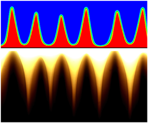
Instability develops somewhat differently at high magnetic fields. As seen from figure 10, the edge peaks grow so rapidly that this process, spreading from the edges to the centre, gradually covers the entire container (figure 10a–f). However, the distance between adjacent peaks in the central part of the container is still somewhat smaller than at the edges. Attention is drawn to the fact that, after the primary peaks have formed, smaller satellites appear between them (figure 10g–j). Their occurrence is associated with a complex flow structure between the main peaks. An upward flow forms in the centre of the main peaks, and a downward one forms along the diffusion front on the outer side of the peaks. This downward flow, reaching the bottom of the container, breaks up into secondary flows and is the cause of the appearance of numerous secondary vortices. As a result, as can be seen from figure 10(i,j), between the main peaks, the occurrence of one, two or three additional peaks is possible. Over time, these peaks disappear as a result of diffusion–advective mixing of fluids.

Figure 10. Development of instability in a high magnetic field for c ₀ = 0.34, H = 0.5, Ra_m = 10⁵, Sc = 10⁵, ${K_H} = f(H)HR{a_m} = 25\;000$, L_x = 1500, L_y = 100, h = 25, Nx = 3000, Ny = 300, Δt = 2.598 × 10⁻⁷: (a) t = 2.59 × 10⁻²; (b) t = 4.68 × 10⁻²; (c) t = 9.88 × 10⁻²; (d) t = 0.108; (e) t = 0.125; (f) t = 0.148; (g) t = 0.260; (h) t = 0.546; (i) t = 1.092; (j) t = 1.559.

The dynamics of the development of the instability of the diffusion front is demonstrated by the animation obtained as a result of numerical simulation, attached to this paper. This animation was obtained for the following problem parameters: c ₀ = 0.05, H = 0.054, Ra_m = 200 000, Sc = 170 000. These parameters, as far as possible, correspond to the experimental conditions (Erglis et al. Reference Erglis, Tatulcenkov, Kitenbergs, Petrichenko, Ergin, Watz and Cebers2013). The aspect ratio of the container was 1 : 15, the height of the container was L_y = 150, the thickness of the magnetic fluid layer was h = L_y/4, the number of nodes during the numerical simulation was Nx × Ny = 4500 × 450. Table 1 shows that the reference value for the length is h ₁ = 0.705 μm, i.e. the container height L_y = 150 approximately corresponds to the experimental value L_y = 127 μm. In this case, the average distance between adjacent peaks in the numerical simulation is 65, i.e. 46 μm, while in the experiment (Erglis et al. Reference Erglis, Tatulcenkov, Kitenbergs, Petrichenko, Ergin, Watz and Cebers2013) a value of approximately 20 μm was obtained. However, as will be shown below, the wavelength of unstable perturbations depends significantly on the thickness of the magnetic fluid layer and, with its decrease, can decrease by a factor of 3–5. Since the thickness of the magnetic fluid layer in the experiment (Erglis et al. Reference Erglis, Tatulcenkov, Kitenbergs, Petrichenko, Ergin, Watz and Cebers2013) is unknown, an exact comparison with experimental data is impossible.

5.2 The influence of the Schmidt number

Equation (2.24) shows that the Schmidt number is included only in the non-stationary part of the equation and, therefore, should not affect the critical values of the wavelength, which are determined by setting the equality of the right side of this equation to zero. However, we checked this statement for the case of moderate magnetic fields: H = 0.125, Ra_m = 158 800 and cavity of size L_x = 1000, L_y = 100. The data are presented in table 3. Here, $\langle \lambda \rangle $ is the average wavelength without taking into account the edge sections, σ is the standard deviation. It can be seen that, within the error limits, the wavelength of unstable perturbations is indeed practically independent of the Schmidt number. In further simulations, the Schmidt number is assumed to be 100 000, which corresponds to the typical physical properties of magnetic fluids presented in table 1.

Table 3. Average wavelength versus Schmidt number.

5.3. Influence of the magnetic field on the wavelength

One of the main parameters determining the development of the instability of the contact line of magnetic and non-magnetic fluids (both miscible and immiscible) is the magnitude of the magnetic field. To determine its influence, we set the following problem parameters: Ra_m = 158 800, Sc = 10⁵, h = L_y/4 and two options for container geometry: (i) L_x = 1000, L_y = 100, Nx × Ny = 2000 × 300; (ii) L_x = 1500, L_y = 100, Nx × Ny = 3000 × 300. Figure 11 shows that the results of both simulations are practically the same, i.e. the influence of edge effects is insignificant.

Figure 11. Dependence of the wavelength on the magnitude of the magnetic field. Squares, L_x = 1000; circles, L_x = 1500. Error bars show σ.

It is noteworthy that the wavelength decreases with increasing magnetic field, while the linear theory constructed in Erglis et al. (Reference Erglis, Tatulcenkov, Kitenbergs, Petrichenko, Ergin, Watz and Cebers2013) for a layer of magnetic fluid of infinite depth predicts an increase in wavelength with increasing magnetic field; in fact it predicts the increase of wavelength of the fastest-growing mode, to be precise. The range of possible wavelengths increases with the field increase. The fact that bending of the diffusion front should be observed corresponding to perturbations with the fastest-growing wavelength is an assumption. This assumption is reasonable, but it is only an assumption. The reasons for this discrepancy are not clear, it could be, for example, differences in the formulations of the problems: the finite depth of the layer, the influence of the boundaries of the container, nonlinear effects or, most probably, the infinitesimal thickness of the diffusion front in the linear theory. The last assumption is confirmed by the results of Cebers (Reference Cebers1997), who for a close problem showed that smearing of the diffusion front shifts the most dangerous mode to a longer wavelength. The result obtained rather resembles the behaviour of the free interface of a magnetic fluid, on which the Rosensweig instability (Cowley & Rosensweig Reference Cowley and Rosensweig1967) develops upon instantaneous switching on of a magnetic field of various magnitudes (Bashtovoi, Krakov & Reks Reference Bashtovoi, Krakov and Reks1985; Dikansky, Zakinyan & Mkrtchyan Reference Dikansky, Zakinyan and Mkrtchyan2010; Zakinyan, Mkrtchyan & Dikansky Reference Zakinyan, Mkrtchyan and Dikansky2016). With an increase in the value of the switched-on magnetic field, the length of the most rapidly developing wavelength in this case significantly decreased. This result was consistent with the linear theory, in which the dispersion equation is determined by both the magnitude of the magnetic field and the surface tension and thickness of the magnetic fluid layer. However, in the problem considered in this paper, there is no surface tension, so that direct analogies with the results of Bashtovoi et al. (Reference Bashtovoi, Krakov and Reks1985), Dikansky et al. (Reference Dikansky, Zakinyan and Mkrtchyan2010) and Zakinyan et al. (Reference Zakinyan, Mkrtchyan and Dikansky2016) are impossible. We will return to the discussion of this analogy below.

In the simulations performed for H ≤ 0.015, a wave-like distortion of the diffusion front was observed only near the side boundaries of the container (similar to figure 10a), the rest of the line of contact of the liquids remained flat throughout, while advective cells (similar to figure 8a) of very low intensity were observed which did not lead to surface distortion. Thus, it is obvious that there is a threshold value of the magnetic field below which the instability of the diffusion front is not observed. However, we cannot assert that this threshold value is 0.015, since, with a decrease in the magnetic field, the development of instability slows down and this leads to an increase in run time. For example, the run time in the case of H = 0.015 was more than three months and the process was stopped due to the low probability of detecting wave formation at the interface between the fluids.

5.3. Wavelength dependence on fluid properties

The influence of the properties of miscible magnetic and non-magnetic fluids is described by the Rayleigh magnetic number. Since the last term in (2.24), which is the source of advective flows, is proportional to both the magnetic field and the magnetic Rayleigh number, it can be expected that the λ(Ra_m) dependence will be qualitatively similar to the λ(H) dependence. The simulation was performed for the parameters H = 0.5, Sc = 10⁵, in the range of values of the magnetic Rayleigh number from 5000 to 200 000. We used the same two options for the geometry of the container and the mesh as in the study of the dependence on the magnetic field. Indeed, figure 12 shows that the wavelength decreases with increasing magnetic Rayleigh number. However, since the magnetic field H = 0.5, chosen to cover the widest possible range of parameter values, is large, and at large Ra_m values, waves of different lengths simultaneously develop at the diffusion front, the spread of λ values in this case turns out to be much larger. The ratio $\sigma /\langle \lambda \rangle $ for Ra_m > 130 000 reached 84 %, and this scatter is especially large in the case of L_x/L_y = 15.

Figure 12. Wavelength dependence on the magnetic Rayleigh number. Squares, L_x = 1000; circles, L_x = 1500. Error bars show σ.

5.4. Dependence of the wavelength on the complex parameter

Since the last term in (2.24), which is the source of advective motion, takes into account the nonlinear nature of the dependence of the magnetization on the magnitude of the magnetic field strength, i.e. is proportional not only to H, Ra_m, but also to f(H), then a complex parameter ${K_H} = f(H)HR{a_m}$ can be introduced, which is their product. In the investigated range of parameters (H < 0.5, Ra_m < 200 000, 102 < K_H < 50 000), all data are in good agreement with a single curve (figure 13).

Figure 13. The dependence of the wavelength on the complex ${K_H} = f(H)HR{a_m}$. Squares, L_x = 1000; circles, L_x = 1500. Error bars show σ.

5.5. The nature of the instability of the diffusion front

As in the development of Rosensweig's instability (Cowley & Rosensweig Reference Cowley and Rosensweig1967; Bashtovoi et al. Reference Bashtovoi, Krakov and Reks1985; Dikansky et al. Reference Dikansky, Zakinyan and Mkrtchyan2010; Zakinyan et al. Reference Zakinyan, Mkrtchyan and Dikansky2016), which arises on the free surface of the magnetic fluid, peaks form at the diffusion front, the distance between them decreasing with increasing magnetic field. This can lead to the conclusion that the instability under study is a complete analogue of Rosensweig's instability. However, there are several fundamental differences between them. In the case of Rosensweig's instability, the wavelength of the most unstable perturbations is determined by the relation $\lambda = 2{{\rm \pi} }\sqrt {\alpha /\mathrm{\Delta }\rho g} $, where α is the surface tension, Δρ is the difference in the densities of the contacting fluids. This wavelength, firstly, does not depend on the thickness of the magnetic fluid layer (Bashtovoi Reference Bashtovoi1978) and, secondly, it increases with increasing surface tension α. Let us consider the influence of these factors for the instability under study.

The dependence on the layer thickness was investigated for the parameters corresponding to the magnetic fluid based on kerosene, for which the experiment was carried out described below (table 1): Sc = 2.56 × 10⁵, Ra_m = 5.59 × 10⁵, χ ₀ = 2.4, c ₀ = 0.41, H = 0.03. The container has dimensions L_x = 1000, L_y = 100, the thickness of the magnetic fluid layer was 6.25, 12.50, 18.75, 25, 35, 50. The data presented in figure 14 show that, when the layer thickness is less than 18, the wavelength of unstable disturbances decreases from 30 to 14. It can be assumed that, perhaps, with a higher container height, the wavelength will also increase. However, we were unable to perform the corresponding simulations due to a significant increase in run time with increasing container size and the need to maintain the distance between nodes h_x = 0.5, h_y = 0.3 to ensure the accuracy of the simulations.

Figure 14. Average wavelength versus layer thickness. Error bars show σ.

Simulation of the instability of a thin layer of liquid was also carried out, with properties corresponding to the data of Erglis et al. (Reference Erglis, Tatulcenkov, Kitenbergs, Petrichenko, Ergin, Watz and Cebers2013) (table 1). In contrast to the version shown in the animation and discussed above, the thickness of the magnetic fluid layer was h = 9. In this case, the average wavelength was λ = 26, which is significantly lower than the value of 65 obtained for a layer with a thickness of 37. Note that the value of the wavelength λ = 26 for this liquid corresponds to the dimensional value of 26 × 0.705 = 18.3 μm, which practically coincides with the experimental data (Erglis et al. Reference Erglis, Tatulcenkov, Kitenbergs, Petrichenko, Ergin, Watz and Cebers2013).

It is usually assumed that there is no surface tension at the diffusion boundary of miscible fluids. However, there is a hypothesis of Korteweg (Reference Korteweg1901), who suggested that a non-uniform density (concentration or temperature) distribution leads to stresses in a fluid. Zeldovich (Reference Zeldovich1949) considered the problem of an effective interfacial tension for such systems and derived an expression for this tension

(5.1)\begin{equation}\alpha = k\frac{{{{(\Delta c)}^2}}}{\delta },\end{equation}

where k is a system-specific parameter, Δc is the variation of mass fraction through the mixing zone and δ is the width of that zone. Although the coefficient k is unknown, the applicability of this hypothesis in the case of magnetic fluids is easy to assess. For highly concentrated microdroplet aggregates arising in a magnetic fluid (Bacri, Salin & Massart Reference Bacri, Salin and Massart1982; Ivanov Reference Ivanov2019), the surface tension is estimated as $1.5 \times {10^{ - 7}}\;\textrm{N}\;{\textrm{m}^{ - 1}}$. The boundary of a microdroplet aggregate, in which the concentration of magnetic particles is almost two orders of magnitude higher than in the surrounding fluid, can be considered to be similar to the diffusion front. Since the concentration of particles in a magnetic fluid is lower than in micro-droplet aggregates, the surface tension (if it exists) can be estimated as $\alpha \sim {10^{ - 7}}\;\textrm{N}\;{\textrm{m}^{ - 1}}$. Since the difference between the densities of the magnetic fluid and the base fluid can be considered equal to Δρ ~ 100 kg m⁻³, the wavelength when Rosensweig's instability occurs should be equal to $\lambda = 2{{\rm \pi} }\sqrt {\alpha /\mathrm{\Delta }\rho g} \approx 60\;\mathrm{\mu }\textrm{m}$. Obviously, in order of magnitude, this value corresponds to both experimental data and our simulations, so that an analogy with Rosensweig's instability can be considered as possible.

However, according to the Korteweg--Zel'dovich hypothesis, with an increase in the width of the diffusion layer δ the effective surface tension coefficient α should decrease. Then, if the analogy with Rosensweig's instability is valid, the wavelength of unstable perturbations $\lambda = 2{{\rm \pi} }\sqrt {\alpha /\mathrm{\Delta }\rho g} $ should also decrease. To analyse this situation, an instability simulation was performed for the following parameter values: H = 0.5, Ra_m = 10⁵, Sc = 10⁵, χ ₀ = 2, c ₀ = 0.34, L_x = 1500, L_y = 100, h = 25, h_x = 1/2, h_y = 1/3. At the initial moment of time, the concentration distribution along the y coordinate was specified in accordance with expression (4.6a) for the moments of time t = 0.001, 0.010, 0.016, 0.036, 0.600, 0.700, 0.920, 2.0, 3.0, 4.0, 6.0, 20.0. Note that, for fluids with moderate viscosity (water, kerosene), as can be seen from table 1, even the maximum time t = 20 corresponds to several seconds of contact time of the miscible magnetic and non-magnetic fluids. The diffusion front width was calculated as the distance between points with a concentration of 0.339 and 0.001. This width was, corresponding to the values of t, the following values: 0.30, 0.78, 1.50, 3.0, 4.5, 6.0, 7.5, 11.0, 13.4, 15.5, 19.0, 34.8. Figure 15 shows that, with an increase in the initial width of the diffusion layer, the wavelength of unstable perturbations increases almost linearly from 40 to 93, while if the analogy with Rosensweig's instability were valid, then the wavelength should decrease. Note that, as will be shown below, in the experiment, the distance between the peaks also increases with the thickness of the diffusion front. This fact confirms that the constructed model without surface tension adequately describes the instability of the diffusion front.

Figure 15. Wavelength vs diffusion front width. Error bars show σ.

Thus, we can conclude that the analogy with the Rosensweig instability does not explain the formation of peaks at the interface of mixing magnetic and non-magnetic fluids in a magnetic field, which occurs on the basis of the balance of gravitational forces, diffusion fluxes and magnetic field energy.

6. Experimental results and discussion

In experimental studies, a magnetic fluid was used, which is a dispersion of magnetite nanoparticles in kerosene, stabilized with oleic acid. The properties of the magnetic fluid are presented in table 1. The magnetic properties of the fluid were obtained with a Lake Shore Cryotronics 7410 VSM vibrating sample magnetometer, density was measured with a Termex vibrating density meter and viscosity with a Rheotest RN 4.1 rotational viscometer. The diffusion coefficient of nanoparticles was measured using a Photocor Complex dynamic and static light scattering spectrometer.

The magnetic fluid was placed in a thin flat cell made of two rectangular transparent Plexiglas plates. The cell width was 25 mm, the height was 15 mm and the distance between the plates was 0.19 mm. The cell was installed vertically. The introduction of liquids into the cell was carried out using a syringe, through which a slow inflow of liquid was carried out simultaneously from the upper left and right edges of the cell. The liquid supplied through the syringe was drawn into the cell due to the capillarity effect. First, a magnetic fluid was introduced, and then kerosene, which was spread over the magnetic fluid during retraction into the cell. As a result of the described procedure, the boundary of liquids with an initially non-zero thickness of the diffuse transition layer between them was obtained. With each new filling of the cell, the thickness of the diffuse layer was reproduced well and amounted to ≈100 μm. To obtain higher values of the diffuse layer thickness, a subcritical magnetic field was applied perpendicular to the liquids’ interface. The duration of the field exposure was varied to obtain different values of the diffuse layer thickness. It should be noted that this procedure for varying the thickness of the diffuse layer has a low reproducibility of the results obtained. Therefore, in the experiments, the actual thickness of the diffuse layer at the moment was determined each time and then the corresponding experiment was performed. The thickness of the kerosene layer in the experiments was always much greater than the thickness of the magnetic fluid layer. As a result, a horizontal quasi-two-dimensional interface of a magnetic fluid and a pure dispersion medium was formed. The cell was placed in a uniform magnetic field directed vertically and generated by Helmholtz coils. Observation of the dynamics of the boundary between magnetic and non-magnetic fluids was carried out using an optical microscope. The installation sketch is shown in figure 16.

Figure 16. Sketch of the experimental set-up.

When the magnetic field was turned on, the settling time to the specified value did not exceed 0.01 s. After switching on the magnetic field, the boundary of the magnetic and non-magnetic fluids was deformed, then peaks appeared on it, directed from the magnetic fluid towards the non-magnetic medium. The peaks formed at the initial moment could then divide, splitting into smaller structures resembling a system of needles in shape. The formation of the peaks was accompanied by intense mixing of the liquids, as a result of which these peaks ultimately dissolve, forming a horizontally uniform transition layer between the magnetic and non-magnetic fluids. The parameters of the developing instability (wavelength, peak growth rate, etc.) substantially depend on the magnitude of the magnetic field, the thickness of the diffuse transition layer between fluids δ and the depth of the magnetic fluid layer. As an example, photographs of the change in the shape of the diffusion front at various parameters of the system are shown in figure 17. The dynamics of the developing instability at various values of the magnetic field is illustrated in the attached movie. The observations were carried out in the central part of the cell, and the occurring instability developed simultaneously over the entire section of the liquid boundary under consideration. In this case, the scales of the occurring structures were significantly less than the cell dimensions, which indicates the possibility of neglecting the edge effects in further analysis.

Figure 17. Evolution of the boundary of mixing magnetic and non-magnetic fluids in a normal magnetic field: (a) a wide diffuse layer, H = 11 kA m⁻¹, δ = 1.2 mm; (b) narrow diffuse layer, H = 5.8 kA m⁻¹, δ = 0.1 mm. The results are for the semi-infinite magnetic fluid layer.

Quantitative estimation of the thickness of the diffuse transition layer between fluids and the depth of the magnetic fluid layer was carried out on the basis of the obtained photographic images. For this, the image was converted to a grey scale format, the area of the image occupied by white pixels was identified with a non-magnetic fluid, the area occupied by black pixels was identified with a magnetic fluid of the initial concentration and the area of pixels with intermediate intensity values corresponded to the transition diffuse layer. The depth of the fluid layer was measured from the bottom of the cuvette to the beginning of the diffuse layer (figure 18). Note that the minimum value of the diffuse layer thickness in the experiments was 0.1 mm.

Figure 18. Method for determining the thickness of the diffuse front and the depth of the magnetic fluid layer.

The minimum thickness of the diffusion front achieved in the experiment (100 μ ≈ 83h ₁) is much greater than the maximum thickness of the diffusion front in the numerical simulation (20 h ₁). Therefore, it is impossible to quantitatively compare the experimental data with the results of numerical simulation. The main focus was on their qualitative comparison and congruence.

It was found that there is a threshold value of the magnetic field strength at which the development of instability of the interface of mixing magnetic and non-magnetic fluids is possible. As the critical value, such values of the magnetic field strength were chosen at which the deformation of the diffusion front became visually perceptible. It should be noted that, in experiments, the field of a certain value had to be applied abruptly, since a smooth increase in the field led to an increase in the thickness of the diffuse layer and a change in the experimental conditions. Therefore, the critical field was found by sequentially reducing the interval between the value of the field at which the instability does not yet occur and the value of the field at which the interface deformation is distinguishable. The minimum achievable width of such an interval in experiments was 100 A m⁻¹, and the critical field value was selected in the middle of this interval. Measurements were made of the dependence of the critical magnetic field strength on the depth of the magnetic fluid layer and the thickness of the diffuse layer. Note that, at subcritical strengths, there is an intensification of both the mixing of liquids in comparison with diffusion in the absence of a magnetic field and the expansion of the diffusion front, but the interface shape remains visually flat. A similar situation was observed in numerical simulation: at subcritical values of the magnetic field, a system of vortices appeared in the central part of the container, which was not associated with vortices at the edges of the container, but the diffusion front remained flat. This system of vortices facilitates the more rapid expansion of the diffusion front.

Figure 19 shows the dependence of the critical magnetic field strength on the depth of the magnetic fluid layer obtained at minimal diffusion front thickness. This dependence is monotonic. When the depth of the magnetic fluid layer is more than 1 mm, the instability threshold does not depend on the depth. In order to present the data in dimensionless form (figure 19b), the $R{a_m}{\chi _0}{H^2}$ criterion was used, since the critical value of the magnetic field (figure 19a) is small and $f(H) = {\chi _0}H$.

Figure 19. (a) Dimension and (b) dimensionless dependence of the critical value of the magnetic field strength on the depth of the magnetic fluid layer.

With an increase in the thickness of the diffuse front δ, the critical magnetic field strength increases (figure 20). In this case, the depth of the magnetic fluid layer was chosen sufficiently large (much larger than the characteristic scale of the arising boundary disturbances), so that the layer in this case can be considered as semi-infinite.

Figure 20. Dependence of the critical value of the magnetic field strength on the thickness of the diffuse front.

The regularities of the development of instability of the diffusion interface of magnetic and non-magnetic liquids in the supercritical region of values of the magnetic field are studied. The time of development of the instability was measured, which was taken as the time interval from the moment of switching on the magnetic field to the moment when the disturbance of the boundary became visually perceptible. Figure 21 shows the experimental dependences of the development time of instability on the thickness of the diffuse front, obtained at two values of the magnetic field strength. As can be seen from the figure, with an increase in the thickness of the diffuse layer, the development time increases monotonically, and decreases with an increase in the field strength. The depth of the magnetic fluid layer in these experiments was quite large.

Figure 21. Dimensionless dependence of the development time of instability on the thickness of the diffuse front.

The instability wavelength was measured, which was determined from the distance between adjacent peaks. In this case, the initial moment of the development of instability before the onset of fission and dissolution of peaks was considered. The error of the presented experimental data was determined from the results of multiple repetitions of the described experiments and averaging of the obtained values. The resulting relative error ranged from 10 % to 20 %. Figure 22 shows the dependence of the wavelength on the thickness of the diffuse front, obtained at three values of the magnetic field strength. The measurements were carried out at a great depth of the magnetic fluid layer. It can be seen from the figure that the instability wavelength increases with an increase in the thickness of the diffuse front, and also decreases with an increase in the field strength. This result correlates qualitatively with the numerical simulation data presented in figure 15.

Figure 22. Dependence of the instability wavelength on the thickness of the diffuse front at different values of the magnetic field strength.

Figure 23 shows the experimentally obtained dependence of the instability wavelength on the depth of the magnetic fluid layer. In this case, the thickness of the diffuse front was the minimum possible. The wavelength increases with increasing depth of the magnetic fluid layer, which qualitatively agrees with the results of numerical simulation shown in figure 14. The inset in figure 23 shows the dependence of the instability wavelength on the magnetic field strength obtained for the minimum thickness of the diffuse layer and the depth of the magnetic fluid layer equal to 0.1 mm. As for the instability of the free surface of a magnetic fluid bordering on an immiscible medium (Bashtovoi et al. Reference Bashtovoi, Krakov and Reks1985; Dikansky et al. Reference Dikansky, Zakinyan and Mkrtchyan2010; Zakinyan et al. Reference Zakinyan, Mkrtchyan and Dikansky2016), this dependence also has a decreasing character. The presented result is in agreement with the simulation data shown in figure 11.

Figure 23. Dependence of the instability wavelength on the depth of the magnetic fluid layer at H = 1.6 kA m⁻¹. Inset: dependence of the instability wavelength on the magnetic field strength at h = 0.1 mm and δ = 0.1 mm.