2.1. Description of the transparent mock-ups

The technique employed for the visualization of the wetted surface during the experiments is based on the use of transparent mock-ups and a LED edge-lighting technique. Three transparent shells of different shapes were built: a circular disc, a cone and a hemisphere. Note that each mock-up corresponds to an axisymmetric transparent shell which was manufactured in a block of PMMA and finely polished. An array of high-power LEDs was mounted at the periphery of each mock-up in order to diffuse light in the material. The LED array was covered of aluminium cellotape in order to maintain it in position and to direct the light toward the mock-up. A vertical cross-section and a picture of each mock-up is displayed in figure 3. In figure 3(a), one can see that the circular disc is composed of a 40 cm central region which is 15 mm thick and a sloped region at the periphery of the mock-up which is 11 mm thick. The disc was continued obliquely with a slope of $30^{\circ }$ in order to prevent the LEDs from being in contact with the water. The conical mock-up described in figure 3(c) is composed of a central part with a deadrise angle of $15^{\circ }$ and a thickness of 15 mm. For the same reason as in the case of the disc, the conical mock-up was continued obliquely with a $30^{\circ }$ tilted edge of 12 mm thickness. The spherical mock-up shown in figures 3(e) and 3(f) corresponds to a truncated hemispherical shell with an external radius of curvature of 353.6 mm and a thickness of 15 mm. In contrast to the other mock-ups, the spherical mock-up was continued tangentially by 40 mm. The extrapolated sides of each mock-up were covered with an aluminium cellotape because of the bad quality of the polishing in these regions. The cellotape acted as a light guide which increased the diffusion of light in the shell and limited the direct lighting of the free surface by the diffusive peripheral regions of the mock-ups. Note that in Tassin et al. (Reference Tassin, Breton, Forest, Ohana, Chalony, Le Roux and Tancray2017), it was not necessary to cover the periphery of the mock-up by aluminium cellotape thanks to the good quality of the polishing. The edge of the mock-ups in contact with the LEDs was roughened to homogenize the light diffusion in the material.

Figure 3. Description of the different mock-ups used in the experiments. (a) Description of the circular disc. (b) Photograph of the disc. (c) Description of the circular cone. (d) Photograph of the cone. (e) Description of the sphere. (f) Photograph of the sphere.

2.2. Compensation of optical distortion

In the case of the three-dimensional mock-ups (cone, sphere), it was necessary to compensate for the optical distortion due to the perspective effects (mainly). In order to do so, we manufactured calibration parts over which the projection of a regular grid was printed. These parts were placed in contact with the lower face of the mock-up (see figure 4) and an image of the grids seen through the mock-up was recorded with the video camera before the series of experiments (see figure 5a). The localization of the intersections between the vertical and horizontal lines in the calibration images was performed with an in-house algorithm developed for the detection of the intersections. A comparison of the measured and theoretical positions of the grid intersections in the case of the cone is shown in figure 5(b). The intersection-point positions were then used to identify an eighth-order polynomial correction model (see Tang et al. Reference Tang, von Gioi, Monasse and Morel2017) of the following form:

(2.1)\begin{equation} \begin{cases} x_2= a_1 x_1^8 + a_2 x_1^7 y_1 + \cdots+ a_{44} y_1 + a_{45} \\ y_2= b_1 x_1^8 + b_2 x_1^7 y_1 + \cdots+ b_{44} y_1 + b_{45} \end{cases} \end{equation}

where ($x_1,y_1$) are the positions of the pixels as observed by the camera and ($x_2,y_2$) are the corrected positions of the points in the $x$–$y$ plane. The value of the parameters of the correction model ($a_1,\ldots , a_{45}, b_1,\ldots , b_{45}$) were adjusted using an optimization algorithm based on the minimization of the distance between the measured and theoretical position of the calibration grid intersections. The absolute residual error maps after calibration for the cone and for the sphere are displayed in figures 5(c) and 5(d), respectively. One can see in figures 5(c) and 5(d) that the average residual error after calibration is lower than one millimetre, except near the centre of the cone where the error reaches 2 mm. The higher error near the centre of the cone can be explained by the presence of manufacturing imperfections at the centre of the cone which affect the accuracy of the intersection detection algorithm. We verified a posteriori that the distortion was negligible in the case of the circular disc (a calibration part was also manufactured for this mock-up).

Figure 4. Calibration part manufactured for the sphere.

Figure 5. Compensation of optical distortion method. (a) Calibration grid seen through the cone with reversed contrast. (b) Comparison between the theoretical position of the intersections (large green crosses) and the detected crosses (small red crosses) from panel (a). (c) Residual error after calibration of the cone. (d) Residual error after calibration of the sphere.

2.3. Initial position of the mock-up

The adjustment of the initial position of the mock-ups in terms of altitude and horizontality is an important feature of the experimental methodology. Different approaches were used for the flat mock-up (circular disc) and the three-dimensional mock-ups (cone and sphere). In the case of the circular disc, the horizontality of the mock-up was first adjusted using an inclinometer ($0.05^{\circ }$ resolution) laying on the upper surface of the mock-up. Then the mock-up was lowered vertically step by step until it touched the still water. The mock-up became fully wetted within a final step of 0.5 mm. This final position was used as the initial position for all the water exit experiments carried out with the circular disc. Note, however, that the initial radius of the wetted surface was greater than the flat part of the mock-up because of the presence of a meniscus wetting a portion of the sloped part of the mock-up (see figure 6a).

Figure 6. Illustration of the meniscus. (a) Circular mock-up. (b) Conical mock-up.

A different approach was used for the adjustment of the ‘horizontality’ of the three-dimensional mock-ups due to the absence of a horizontal plane surface to place the inclinometer. In this case, the mock-up was first partially wetted and then the horizontality was adjusted in order to obtain a symmetric wetted surface (for this purpose, an image of the calibration grid was superimposed to the image of the camera). Finally, the vertical position of the mock-up was adjusted to obtain the desired value of the wetted surface radius. This position was used as the reference position in the water exit and entry–exit experiments. Note that, with this methodology, the size of the wetted surface is influenced by the presence of the meniscus. This means that the boundary of the wetted surface does not correspond to the intersection of the still water surface with the lower surface of the mock-up (see figure 6b).

2.4. Motion prescribed to the mock-up

In the water exit experiments, the elevation of the mock-up, $h(t)$, with respect to its initial position follows the following time evolution:

(2.2)\begin{equation} \begin{cases} h(t)=H[1+\mathrm{erf}(U_{max}(t-t_0)\sqrt{\rm \pi}/H)]/2, & t \leq t_0, \\ \dot{h}(t)=U_{max}, & t \geq t_0 , \end{cases} \end{equation}

with $\mathrm {erf}(x)=(2/\sqrt {{\rm \pi} }) \int _0^x \exp (-\tau ^2) \, \mathrm {d}\tau$ the error function, $U_{max}$ the maximum velocity reached during the experiment, $H$ the maximum elevation of the mock-up and $\dot h(t)$ the time derivative of $h(t)$. In the water exit experiments, the value of $H$ was fixed to 10 cm, the value of $U_{max}$ was varied from 0.2 to $0.6\ \textrm {m}\,\textrm {s}^{-1}$ and $t_0$ was set to 3 s. The time history of the velocity and acceleration for the different values of $U_{max}$ is illustrated in figure 7. Formally speaking, $h(t)$ tends to 0 at $t=-\infty$, but in practice $h(0)$ was considered to be sufficiently small to be neglected in the experiments. Note that this motion was inspired by Reis et al. (Reference Reis, Jung, Aristoff and Stocker2010) who originally studied the water exit phenomenon in order to understand the cat lapping phenomenon. Following Reis et al. (Reference Reis, Jung, Aristoff and Stocker2010), the characteristic speed $U_{max}$ and the initial wetted surface radius $c_0$ can be used to calculate the Froude (Fr), Reynolds (Re) and Weber (We) numbers for the water exit experiments: $\textit {Fr}=U_{max}/\sqrt {g c_0}$, ${Re}=U_{max} c_0/\nu$ and ${We}=\rho c_0 U_{max}^2 /\sigma$, with $g$ the acceleration due to gravity, $\nu$ the liquid kinematic viscosity and $\sigma$ the surface tension coefficient. In the water exit experiments, the value of $Fr$ ranges from 0.13 ($U_{max}=0.2\ \textrm {m}\, \textrm {s}^{-1}$, $c_0=0.25$ m) to 0.43 ($U_{max}=0.6\ \textrm {m}\, \textrm {s}^{-1}$, $c_0= 0.2$ m), $Re \approx 4.0\times 10^4$ to $1.5\times 10^5$ and $We \approx 1.1\times 10^2$ to $1.2\times 10^3$.

Figure 7. Evolution of the velocity (a) and acceleration (b) as a function of time during the water exit experiments for different values of $U_{max}$.

In the water entry and exit experiments, the elevation of the lowest point of the mock-up, $h(t)$, with respect to the free-surface altitude follows the following time evolution:

(2.3)\begin{equation} \begin{cases} h(t)=-(H/2)\cdot \mathrm{erf}(U_{max}(t-t_0)\sqrt{\rm \pi}/H), & t \leq t_0, \\ h(t)=-H\sin(2{\rm \pi}(t-t_0)/T), & t_0 \leq t \leq T/2 + t_0,\\ \dot{h}(t)=U_{max}, & t \geq T/2 + t_0 \end{cases} \end{equation}

with $U_{max}$ the maximum velocity and $T=2{\rm \pi} H/U_{max}$; $H$ is the maximum submergence depth and $t_0=3$ s. The body enters the water at $t_0$ with an initial velocity equal to $-U_{max}$. The acceleration is maximum at $t=T/4+t_0$ when the body begins to move upward. Note that for $t \le t_0$, the motion prescribed to accelerate the mock-up to the desired entry velocity follows the same evolution as for the exit experiments, but in the downward direction. Using the axisymmetric formulation of Wagner's theory, $H$ can be related to $c_{max}$, the maximum wetted surface radius expected to be reached in an experiment. For the $15^{\circ }$ cone, the Wagner condition (see Korobkin & Scolan Reference Korobkin and Scolan2006, equation (48)) reads: $H={\rm \pi} \tan (15 ^{\circ })c_{max}/4$ and for the sphere: $H=\int _0^{{\rm \pi} /2} \sin \beta [R-\sqrt {R^2-c_{max}^2\sin ^2\beta } ] \,\textrm {d} \beta$, where $R=353.6$ mm. The values of the maximum acceleration attained during the different combined entry and exit experiments are reported in table 1. The Froude, Reynolds and Weber numbers can be calculated in a similar way as for the exit experiments, except that $c_0$ should be replaced by $c_{max}$. The values of $Fr$ corresponding to the experiments are given in table 1.

Table 1. Froude number and maximum acceleration attained during the combined entry and exit experiments for the different values of $c_{max}$ and $U_{max}$.

3.1. Synchronization of the measurements with the motion generator

The data acquisition system and the high-speed video camera were triggered by the same signal coming from the motion generator, and so were well synchronized to each other with a maximum time shift of 1 ms (the sampling frequency and frame rate were both set to 1 kHz). However, it was not possible to accurately synchronize the motion of the hexapod and the data/video acquisition system during the experiments. In our analysis of the experiments, we compared the theoretical acceleration evolution and the recorded acceleration signal to ‘re-synchronize’ the measurements with the motion. The time shift between the motion and the measured signals was obtained by maximizing the cross-correlation between the measured and theoretical acceleration signals. In order to do so, we filtered the high-frequency oscillations of the measured acceleration signals using a Fourier low-pass filter with a cutoff frequency of 30 Hz. An example of the raw and filtered acceleration signals measured during a water exit experiment with $U_{max}=0.6\ \textrm {m}\, \textrm {s}^{-1}$ is depicted in figure 8. A comparison of the theoretical and measured acceleration signals is presented in figure 9. The theoretical acceleration signal after applying the same low-pass filter is also depicted in figure 9 to show that the filtering operation does not affect the dynamics of the motion. We can see that the hexapod follows quite well the target motion even if the measured acceleration exhibits a small oscillation which leads to a difference of about $0.28\ \textrm {m}\, \textrm {s}^{-2}$ in terms of the acceleration peak value. Despite the small oscillations of the acceleration signal, the motion of the hexapod is very repeatable as it can be seen in figure 10 where we compare the filtered acceleration signals recorded during three experiments of exit in air with $U_{max}=0.6\ \textrm {m}\, \textrm {s}^{-1}$.

Figure 8. Comparison of the original and filtered measured acceleration signals during a water exit experiment with $U_{max}=0.6\ \textrm {m}\, \textrm {s}^{-1}$.

Figure 9. Comparison of the filtered measured and target acceleration (filtered and unfiltered) for water exit with $U_{max}=0.6\ \textrm {m}\, \textrm {s}^{-1}$.

Figure 10. Comparison of the measured acceleration signals for three similar exit experiments in air with $U_{max}=0.6\ \textrm {m}\, \textrm {s}^{-1}$.

3.2. Tracking of the contact line

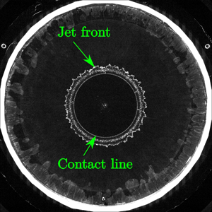
A sequence of four images recorded during the water entry and exit of the cone for different time instants is plotted in figure 11. During the entry stage (figures 11a and 11b), both the jet front and the contact line are clearly visible. Indeed, they are both illuminated by the LED edge-lighting system. During the exit stage (figures 11c and 11d), the jet disappears but the contact line, which contracts towards the centre, is still clearly visible. Some additional concentric luminous rings are nevertheless visible in figures 11(c) and 11(d). These features are imparted to undesired specular reflections of the very bright outer region of the mock-up on the free surface, but their presence does not alter the tracking of the contact line which corresponds to the inner luminous ring in the images. In order to measure the evolution of the contact line during the experiments, the contact line geometry is extracted using a contour detection algorithm based on the method of Taubin (Reference Taubin1991) and assuming that the shape of the contact line is elliptic. The performance of the contour tracking algorithm is illustrated in figure 12 where the detected contours and the original images (from figure 11) are superimposed. The tracking of the contact line is not problematic, except for a very short duration at the moment of the transition between the entry stage and the exit stage because the contact line is not bright enough. In order to verify that the inner ring corresponds to the contour of the wetted surface (the contact line), the same experiments were conducted with a draughtboard laying at the bottom of the tank (approximately 2 m below the free surface). With this technique, the region over which the water is in contact with the mock-up corresponds to the region over which the draughtboard appears undistorted (except for the optical distortion due to the shape of the mock-up), as shown in figure 13. The red dashed line, which is superimposed on the images obtained with the draughtboard technique in figure 13, corresponds to the contour extracted from figure 12. One can observe that the region over which the draughtboard remains undistorted is perfectly circumscribed by the contour extracted from figure 12. This comparison demonstrates the accuracy of the LED edge-lighting technique for both water entry and water exit experiments. A more detailed validation of the LED edge-lighting technique through comparison with images obtained with the draughtboard technique for the different mock-ups is presented in appendix A.

Figure 11. Sequence of images obtained during the water entry (a,b) and exit (c,d) of the cone with $c_{max}=250$ mm and $U_{max}=0.6\ \textrm {m}\, \textrm {s}^{-1}$: ($a$) $t=3.036$ s, ($b$) $t=3.073$ s, ($c$) $t=3.166$ s and ($d$) $t=3.318$ s.

Figure 12. Tracking of the contact line during the water entry (a,b) and exit (c,d) of the cone: ($a$) $t=3.036$ s, ($b$) $t=3.073$ s, ($c$) $t=3.166$ s and ($d$) $t=3.318$ s.

Figure 13. Comparison between the contact line obtained with the LED edge-lighting technique (red dashed line) and the images obtained with the draughtboard during the water entry and exit of the cone: ($a$) $t=3.036$ s, ($b$) $t=3.073$ s, ($c$) $t=3.166$ s and ($d$) $t=3.318$ s.

3.3. Hydrodynamic force measurement

In our analysis procedure, the force signals are first low-pass filtered with the same filter as the acceleration signal. It was shown previously that the filtering operation did not affect the acceleration signal (see figure 9). Given that the hydrodynamic force during water exit is principally due to an ‘added mass-like’ effect (see Tassin et al. Reference Tassin, Jacques, El Malki Alaoui, Nême and Leblé2012; Korobkin Reference Korobkin2013), we can anticipate that the filtering will not affect the force signals (except for the removal of the high-frequency oscillations). The force measured by the sensors is a combination of the action of the water on the mock-up and the inertia force due to the mass of the mock-up and of the mechanical parts connecting the mock-up to the force sensors. In order to subtract the force component due to inertia from the total measured force, the inertia component was measured by running experiments in air with a motion identical to the experiments with water. Each experiment in air and water was repeated three times with the same prescribed motion. The measured total force and the contribution of the different force components during an experiment of water entry and exit with the cone are plotted in figure 14(a). One can appreciate the relative importance of the inertia component ($F_{inertia}$) to the total force.

Figure 14. Contribution of the different force components to the total force. (a) Water entry and exit of a cone with $U_{max}=0.6\ \textrm {m}\, \textrm {s}^{-1}$ and $c_{max}=250\ \textrm {mm}$. (b) Water exit of a cone with $U_{max}=0.6\ \textrm {m}\, \textrm {s}^{-1}$ and $c_0=250\ \textrm {mm}$.

The use of piezoelectric force sensors, even with a slow-drift charge amplifier like the one we used, requires a reset of the level of reference of the force sensors at the beginning of the experiment. As a consequence, the measured hydrodynamic force is equal to zero at the beginning of the pure exit experiment, even for the three-dimensional mock-ups, despite the action of Archimedes’ force. In the results presented in the following sections, the reset of the force sensors is corrected by subtracting the final asymptotic value of the hydrodynamic force (when the mock-up is fully unwetted and the velocity is null). The contribution of the different force components during the water exit of the cone are shown in figure 14(b).

3.4. Correction of the reference elevation in the water entry and exit experiments

The presence of the meniscus induces an uncertainty of $\delta _z$ (corresponding to the meniscus height) on the initial position of the three-dimensional mock-ups (with respect to the still water level) . However, the height of the meniscus can be estimated from the experiments in two ways. The first way is to find a value of $\delta _z$ such that the theoretical buoyancy force is equal to the measured force at the beginning of the water exit experiment. The second way is to detect from the high-speed videos the time instant when the mock-up touches the water ($t=t_0+\delta _t$) and to compute the theoretical elevation of the mock-up at this time instant ($h(t_0+\delta _t)$). The values obtained for $\delta _z$ with the two approaches for the cone and the sphere are given in tables 2 and 3, respectively. One can see that the maximum difference between the two estimates is about 1 mm. Note that these values will be used later in order to make comparisons with the theoretical results.

Table 2. Estimation of the meniscus height $\delta _z$ for the cone: $\delta _z^*$ is the estimate of $\delta _z$ based on the measured value of Archimedes’ force and $|h(t_0+\delta _t)|$ is the estimate of $\delta _z$ based on the measured value of $\delta _t$.

Table 3. Estimation of the meniscus height $\delta _z$ for the sphere: $\delta _z^*$ is the estimate of $\delta _z$ based on the measured value of Archimedes’ force and $|h(t_0+\delta _t)|$ is the estimate of $\delta _z$ based on the measured value of $\delta _t$.

4.1. Evolution of the wetted surface and of the hydrodynamic force during the water exit experiments

The evolution of the radius of the wetted surface during the water exit of the circular disc is depicted in figure 15 for different values of the maximum exit velocity. The corresponding force evolutions are presented in figure 16. One can observe in figure 15 that the evolution of the wetted surface radius depends on the exit velocity. For a given disc elevation, the radius is smaller when the velocity is decreased. This phenomenon is due to the action of the gravity. As the maximum exit velocity decreases, the peak (absolute) value of the hydrodynamic force decreases and occurs earlier.

Figure 15. Evolution of the radius of the wetted surface as a function of the elevation during the water exit of the circular disc for different values of $U_{max}$.

Figure 16. Evolution of the hydrodynamic force as a function of time during the water exit of the circular disc for different values of $U_{max}$.

The results obtained with the cone are depicted in figures 17 and 18. Similarly to the circular disc, the reduction of the wetted surface radius with the elevation is more pronounced as the velocity decreases. In figure 17, the evolution of the radius of the wetted surface obtained with a von Karman approach is also plotted. Within the von Karman approach, the contact line position is determined as the intersection between the body surface and the reference horizontal plane $z=\delta _z$ (represented by a black dotted line in figure 6b). The difference between the experimental results and the results obtained with the von Karman approach illustrates the pile-up of the free surface induced by the water exit. The hydrodynamic force evolutions measured during the water exit of the cone differ from that measured during the water exit of the circular disc due to the static buoyancy of the cone. The buoyancy force mitigates the suction force in the case of the cone. For the lowest velocity ($U_{max}=0.2\ \textrm {m}\, \textrm {s}^{-1}$), the hydrodynamic force remains positive during the entire duration of the exit experiment. In agreement with what can be expected from a theoretical model of exit based on an added mass approach, the hydrodynamic force measured during the water exit of the disc and the cone becomes very low when the acceleration vanishes (at $t = 3\ \textrm {s}$). However, it is not equal to zero. Indeed, a drag force is observed for $t>3\ \textrm {s}$. This force decreases gradually with time, most likely because of the decrease of the size of the wetted surface.

Figure 17. Evolution of the radius of the wetted surface as a function of the elevation during the water exit of the cone for different values of $U_{max}$.

Figure 18. Evolution of the hydrodynamic force as a function of time during the water exit of the cone for different values of $U_{max}$.

The results obtained during the water exit of the sphere are presented in figures 19 and 20. In this case, the velocity has a much smaller influence on the evolution of the radius of the wetted surface. One may expect that the effect of the gravity would be more pronounced in the case of the sphere due to the larger volume displaced by the mock-up, but the difference between the experimental results and the results obtained with the von Karman approach (also plotted in figure 19) demonstrates that the phenomenon is not quasi-static. Also note that the hydrodynamic force remains positive during almost the entire duration of the experiments, even for the highest maximum velocity ($0.6\ \textrm {m}\, \textrm {s}^{-1}$), due to the importance of the buoyancy force.

Figure 19. Evolution of the radius of the wetted surface as a function of the elevation during the water exit of the sphere for different values of $U_{max}$.

Figure 20. Evolution of the hydrodynamic force as a function of time during the water exit of the sphere for different values of $U_{max}$.

4.2. Water entry and exit of the cone

The evolutions of the radius of the wetted surface during the combined water entry and exit of the cone are presented in figures 21 and 22 for $c_{max}=200$ mm and $c_{max}=250$ mm, respectively. The maximum radius, $c_{max}$, corresponds to the theoretical value of the radius of the wetted surface obtained with the Wagner model when the penetration depth is maximum (at $t=t_0+T/4$). Note that the maximum value of $c_{max}$ is not attained during the experiments. We will see later that this can be explained by a value of $\delta _z\approx 3$ mm. The value of the maximum velocity ($U_{max}$) has little effect on the maximum value of the radius of the wetted surface. This indicates that gravity does not affect the wetted surface evolution during the entry stage (for the considered entry velocities). The evolution of the hydrodynamic force for $c_{max}=200$ mm and for $c_{max}=250$ mm is shown in figures 23 and 24, respectively. According to the image recordings, the cone starts touching the water at $t=t_0+\delta _t\approx 3.005\ \textrm {s}$ (see table 2). After that, the load begins to increase and reaches rapidly a maximum. Then, the load decreases and becomes negative (corresponding to suction forces). It should be noted that at the time when the force is equal to zero, the mock-up velocity is still downward. The duration of the stage during which the force is negative is longer than the one during which it is positive. In addition, the maximum force, in terms of magnitude, corresponds to a suction load (directed downward) and is reached at the transition between the entry and exit stages. This observation is in line with the experimental observations and theoretical predictions of Baarholm & Faltinsen (Reference Baarholm and Faltinsen2004) and Tassin et al. (Reference Tassin, Piro, Korobkin, Maki and Cooker2013). Note that the force results measured during the experiments with $U_{max}=0.4\ \textrm {m}\, \textrm {s}^{-1}$ exhibit more oscillations than the results obtained with $U_{max}=0.57\ \textrm {m}\, \textrm {s}^{-1}$.

Figure 21. Evolution of the radius of the contact line as a function of time during the water entry and exit of the cone for $c_{max}=200\ \textrm {mm}$.

Figure 22. Evolution of the radius of the contact line as a function of time during the water entry and exit of the cone for $c_{max}=250\ \textrm {mm}$.

Figure 23. Evolution of the hydrodynamic force as a function of time during the water entry and exit of the cone for $c_{max}=200\ \textrm {mm}$.

Figure 24. Evolution of the hydrodynamic force as a function of time during the water entry and exit of the cone for $c_{max}=250\ \textrm {mm}$.

4.3. Water entry and exit of the sphere

The evolution of the hydrodynamic force during the combined water entry and exit of the sphere is presented in figures 25 and 26 for $c_{max}=200$ mm and $c_{max}=250$ mm, respectively. Note that the cutoff frequency was set to 25 Hz instead of 30 Hz for the results presented in figure 26 in order to reduce the oscillations of the force signal due to the vibrations of the set-up. One can observe that, in contrast to the water entry and exit of the cone, the maximum magnitude of the force is more important during the entry stage than during the exit stage. Due to a weak contrast in the images, it has not been possible to use the automatic contact line tracking algorithm for the entry and exit experiments carried out with the sphere.

Figure 25. Evolution of the hydrodynamic force as a function of time during the water entry and exit of the sphere for two different velocities and a theoretical $c_{max}=200\ \textrm {mm}$.

Figure 26. Evolution of the hydrodynamic force as a function of time during the water entry and exit of the sphere for a theoretical $c_{max}=250\ \textrm {mm}$.

5.1. Effect of the scale (experiments in Froude similarity)

At present, there are still some open questions regarding the mechanisms governing the wetted surface dynamics in water exit problems. In particular, the question of the effect of surface tension and viscosity at the early stage of a water exit event was raised by Korobkin (Reference Korobkin2013). In order to assess the importance of these effects in our experiments, we conducted experiments in Froude similarity with the cone for different values of the initial wetted surface, hence varying the scale of the experiments (so varying the Reynolds and Weber numbers) while keeping the Froude number constant. The initial value of the radius of the wetted surface was varied from $c_0=250$ mm to $c_0=100$ mm. The scaling was based on a reference maximum velocity $U_{max}=0.6\ \textrm {m}\, \textrm {s}^{-1}$, a maximum elevation height $H=0.1$ m and $c_0=0.25$ m. Assuming that $\alpha =c_0/0.25$ (with the value of $c_0$ in metres) represents the scale of the experiment, the function $h(t)$ defining the motion of the cone for the different values of $c_0$ is given by (2.2), with $H=\alpha \times 0.1\ \textrm {m}$, $U_{max}=\sqrt \alpha \times 0.6\ \textrm {m}\, \textrm {s}^{-1}$ and $t_0=\sqrt \alpha \times 3\ \textrm {s}$. The results obtained for the different values of $c_0$ are compared in figure 27 in terms of the non-dimensional radius of the wetted surface as a function of the non-dimensional elevation. One can see that the results obtained at different scales are in very close agreement. Note, however, that the results obtained with $c_0=100$ mm slightly deviate from the others at the end of the exit, but this difference remains within the accuracy margin of the experimental approach because of the imperfections at the centre of the conical mock-up (see figure 5c). These experiments show that the influence of surface tension and viscosity is marginal at the largest scales and that the dynamics of the wetted surface is mainly controlled by inertia and gravity effects. Following the theoretical work of Korobkin et al. (Reference Korobkin, Khabakhpasheva and Rodríguez-Rodríguez2017b) who showed that the quantity $1-c(t)/c_0$ was proportional to $[h(t)/c_0]^{2/3}$ during the water exit of a flat plate at constant acceleration, the experimental results obtained in Froude similarity are depicted in figure 28 in terms of the quantity $1-c(t)/c_0$. One can see that the results compare very well with the power law predicted by Korobkin et al. (Reference Korobkin, Khabakhpasheva and Rodríguez-Rodríguez2017b) (but with a different coefficient) for $h(t)/c_0$ ranging from 0.1 to 0.7. This agreement is somewhat surprising given the influence of gravity in our experiments (see figure 17) and the rather different motion imposed to the cone.

Figure 27. Evolution of the non-dimensional radius of the wetted area $c(t)/c_0$ as a function of the non-dimensional elevation during the water exit of the cone for different values of $c_0$ in Froude similarity.

Figure 28. Evolution of $1-c(t)/c_0$ as a function of the non-dimensional elevation during the water exit of the cone for different values of $c_0$ in Froude similarity with a log–log scale.

5.2. Effect of the exit velocity

In this section, the effect of the exit velocity ($U_{max}$) on the evolution of the contact surface during the water exit experiments is analysed by plotting the quantity $1-c(t)/c_0$ as a function of the non-dimensional elevation $h(t)/c_0$. The results obtained for the disc, the cone and the sphere are plotted in figures 29, 30 and 31, respectively. The experimental results of Vega-Martínez et al. (Reference Vega-Martínez, Rodríguez-Rodríguez, Khabakhpasheva and Korobkin2019) corresponding to the water exit of an elastic circular disc are also shown for comparison in figure 29, but note that their experimental results are limited to $c(t)/c_0 > 0.9$. Two important conclusions can be drawn from these observations. First, the time history of the velocity (for $U_{max}$ sufficiently large), the elasticity and the shape of the body do not seem to affect significantly the evolution of the radius of the wetted surface with the body elevation. Second, the theoretical prediction of Korobkin et al. (Reference Korobkin, Khabakhpasheva and Rodríguez-Rodríguez2017b), which is based on a self-similar small-time expansion, seems to be valid for values of $h(t)/c_0$ as large as 0.7. However, as the value of $U_{max}$ decreases, the power coefficient evolves. This effect, clearly visible for $U_{max}=0.2\ \textrm {m}\, \textrm {s}^{-1}$ in figures 29 and 30, is due to the influence of gravity.

Figure 29. Evolution of $[1-c(t)/c_0]$ as a function of the non-dimensional elevation during the water exit of the disc for different values of $U_{max}$. The plots denoted by $R1$, $R2$, $R3$ and $R4$ correspond to four experimental results obtained by Vega-Martínez et al. (Reference Vega-Martínez, Rodríguez-Rodríguez, Khabakhpasheva and Korobkin2019) with a 10.8 cm radius circular disc.

Figure 30. Evolution of $[1-c(t)/c_0]$ as a function of the non-dimensional elevation during the water exit of the cone for different values of $U_{max}$.

Figure 31. Evolution of $[1-c(t)/c_0]$ as a function of the non-dimensional elevation during the water exit of the sphere for different values of $U_{max}$.

5.3. Effect of the body shape

In the linearized water exit model proposed by Korobkin (Reference Korobkin2013), and further developed in Korobkin et al. (Reference Korobkin, Khabakhpasheva and Maki2017a), the body shape has no effect on the evolution of the wetted surface, provided that the size of the initial wetted surface and the body motion are similar. In order to confirm experimentally this assumption, we compare the results obtained with the different body shapes (circular disc, cone, sphere), but with a similar value of $c_0$ and a similar motion. Figure 32 shows the evolution of the radius of the wetted surface as a function of the elevation $h(t)$ measured during the water exit of the three mock-ups for $c_0=200$ mm. One can see that the evolution of the radius of the wetted surface for the cone and the disc are very close, except that the dewetting of the disc is delayed by a small time shift. This time shift may come from the fact that the initial radius of the wetted surface is slightly larger than 200 mm because of the meniscus. The evolution of the sphere seems to follow the evolution of the cone at the beginning of the experiments and then approaches the evolution of the disc. This comparison shows that the body shape has a marginal effect on the evolution of the wetted surface during water exit. This observation is consistent with the water exit model of Korobkin (Reference Korobkin2013) which is insensitive to the shape of the body exiting water (except for the size of the initial wetted surface). The hydrodynamic force measured during the experiments with the different body shapes is shown in figure 33. The total hydrodynamic force measured with the different mock-ups is largely affected by the importance of Archimedes’ force. The results obtained after subtracting the initial value of the force are also depicted in figure 33 in order to compare the ‘purely dynamic’ contribution with the total hydrodynamic force in the different cases. This comparison shows that the dynamic contribution is rather close for the three shapes at the beginning of the exit (until $t\approx 2,9\ \textrm {s}$).

Figure 32. Effect of the body shape on the evolution of the radius of the wetted area $c(t)$ during water exit experiments ($U_{max}=0.6 \ \textrm {m}\, \textrm {s}^{-1}$ and $c_0=200\ \textrm {mm}$).

Figure 33. Effect of the body shape on the evolution of the hydrodynamic force $F_{hydro}$ during water exit experiments ($U_{max}=0.6 \ \textrm {m}\, \textrm {s}^{-1}$ and $c_0=200\ \textrm {mm}$).

5.4. Effect of the entry stage on the results of the exit stage

In the case of a combined water entry and exit event, the fluid is set in motion and the water free surface is deformed during the entry stage, and one may ask if the exit stage (when it takes place after an entry stage) may differ from a pure water exit experiment. In order to assess the effect of the entry stage on the exit stage, we compare the evolution of the wetted surface during an experiment of pure water exit (for $U_{max}=0.6\ \textrm {m}\, \textrm {s}^{-1}$) and during the exit stage of an experiment of combined water entry and exit (for $U_{max} = 0.57\ \textrm {m}\, \textrm {s}^{-1}$) using the conical mock-up. We can see in figure 34 that, even if the dynamics of the mock-up is not exactly the same in both cases, the evolution of the radius of the wetted surface in the pure-exit experiment is comparable with that observed during the exit stage of a combined water entry and exit experiment. Note that the radius of the wetted surface measured during the combined water entry and exit experiments is non-dimensionalized with respect to the maximum value measured during the experiment. The same results are plotted in logarithmic scale in figure 35. One can observe the very close agreement between the results measured during the exit stage of the combined water entry and exit experiment and the power law predicted by the theory of Korobkin et al. (Reference Korobkin, Khabakhpasheva and Rodríguez-Rodríguez2017b). These observations lead us to the important conclusion that a similar water exit model can be used to model both a pure water exit event and the exit stage of a combined water entry and exit event (e.g. in a $2D+t$ approach such as the one used in Bensch et al. (Reference Bensch, Shigunov, Beuck and Söding2001), see also Tassin et al. (Reference Tassin, Piro, Korobkin, Maki and Cooker2013) and Korobkin et al. (Reference Korobkin, Khabakhpasheva and Maki2017a)).

Figure 34. Evolution of the non-dimensional radius of the wetted surface $c(t)/c_0$ as a function of the non-dimensional elevation $h(t)/c_0$ with $c_0=200\ \textrm {mm}$.

Figure 35. Evolution of the non-dimensional radius of the wetted surface $c(t)/c_0$ as a function of the non-dimensional elevation $h(t)/c_0$ with $c_0=200\ \textrm {mm}$ and in log–log scale.

5.5. Comparison with theoretical results

In this section we compare the experimental results with theoretical results obtained with different analytical models of water entry and exit. In figure 36, the evolution of the wetted surface measured during the water exit experiments with the circular disc is compared with the analytical model of Korobkin et al. (Reference Korobkin, Khabakhpasheva and Maki2017a), which is an extension of the model initially proposed in Korobkin (Reference Korobkin2013) to an arbitrary time evolution of the acceleration of the body. In the axisymmetric version of this model, the hydrodynamic force, $F$, is given by the added mass and the acceleration of the body

(5.1)\begin{equation} F(t)=-\frac{4}{3}\rho c^3(t) \ddot h(t), \end{equation}

and the evolution of the radius of the contact surface, $c(t)$, is governed by the following differential equation

(5.2)\begin{equation} \frac{\textrm{d} c}{\textrm{d} t}=-\frac{2}{\rm \pi}\gamma c(t) \int_{t_1}^{t}\frac{\ddot h (\tau) \,\textrm{d}\tau}{\sqrt{c^2(\tau)-c^2(t)}}, \end{equation}

where $t_1=-\infty$ for the pure water exit experiments and $t_1=t_0+T/4$ in the combined water entry and exit experiments. We follow the methodology proposed in Korobkin et al. (Reference Korobkin, Khabakhpasheva and Maki2017a) to solve (5.2), but once the solution is well initialized, we solve directly (5.2) with a standard first-order explicit Euler integration scheme because the methodology proposed in Korobkin et al. (Reference Korobkin, Khabakhpasheva and Maki2017a) is no longer valid when the body acceleration $\ddot h(t)$ is equal to 0. It is important to have in mind that gravity effects are neglected in this model, but quantitative comparisons with the experimental results can be made during the early stage of the exit. Indeed, the very close agreement between the experimental results obtained for $U_{max}=0.6\ \textrm {m}\, \textrm {s}^{-1}$ and $U_{max} = 0.4\ \textrm {m}\, \textrm {s}^{-1}$ for $h(t)< 30\ \textrm {mm}$ indicates that gravity has very little effect on the evolution of the wetted surface during this stage. The theoretical results obtained with $\gamma =1$ are closer to the experimental results obtained for $U_{max}= 0.6\ \textrm {m}\, \textrm {s}^{-1}$ and $U_{max} = 0.4 \ \textrm {m}\, \textrm {s}^{-1}$ at the beginning of the exit, but the theoretical model overestimates the width of the wetted surface as the elevation increases. This divergence between the theoretical and the experimental results is due to the gravity effect which increases as $h(t)$ increases. With $\gamma =2$, the theoretical model seems to underestimate significantly the width of the wetted surface. From figure 36, it seems that there is a slight shift between the experimental and theoretical (for $\gamma =1$) wetted surface radius evolutions. The reason for that is probably due to the fact that the initial value of the wetted surface in the experiments is slightly larger than the disc radius, because of the presence of a meniscus (see figure 6). The same problem does not occur during the water exit of the cone because the initial altitude of the mock-up was adjusted such as to have the desired value of $c_0$ (see § 2.3). Figure 37 presents a comparison between the predictions of the linearized water exit model of Korobkin et al. (Reference Korobkin, Khabakhpasheva and Maki2017a) and the experimental wetted surface evolutions obtained with the cone for different exit velocities. For low values of the elevation $h(t)$, the evolution of the wetted surface radius is independent of the exit velocity. This corresponds to the stage where gravity effects are negligible. During this stage, the results obtained from the model of Korobkin et al. (Reference Korobkin, Khabakhpasheva and Maki2017a) with $\gamma =1$ are in excellent agreement with the experimental results. In figure 38, we compare the hydrodynamic force measured during the water exit of the circular disc with the hydrodynamic force predicted by the added mass approach (5.1) and using the value of $c(t)$ measured during the experiments. Note that we were not able to measure the width of the wetted surface at the very beginning of the experiments, so we used the first measured value of $c(t)$ to calculate the hydrodynamic force at the beginning of the exit. Figure 38 shows that the added mass approach seems to provide a good prediction of the hydrodynamic force for the largest values of $U_{max}$. For smaller exit velocities, the added mass approach largely underestimates the hydrodynamic force. The reason of these differences is very likely related to the influence of gravity, which is not included in the added mass approach. However, the measured hydrodynamic force still follows a time evolution similar to the time evolution of the acceleration, despite the fact that the magnitude of the body acceleration is much smaller than the gravity acceleration for $U_{max}=0.2\ \textrm {m}\, \textrm {s}^{-1}$ (see figure 7b).

Figure 36. Comparison between the wetted surface radius predicted by the model of Korobkin et al. (Reference Korobkin, Khabakhpasheva and Maki2017a) and the one measured during the water exit of the disc.

Figure 37. Comparison between the wetted surface radius predicted by the model of Korobkin et al. (Reference Korobkin, Khabakhpasheva and Maki2017a) and the one measured during the water exit of the cone.

Figure 38. Comparison between the hydrodynamic force predicted by the linearized added mass approach and the one measured during the water exit of the disc.

In figures 39 and 40, the evolution of the radius of the wetted surface measured during the water entry and exit of the cone is compared with the theoretical prediction of the radius of the wetted surface obtained from the combined Wagner-modified von Karman model. This model was proposed by Tassin et al. (Reference Tassin, Piro, Korobkin, Maki and Cooker2013) for the two-dimensional case and is directly applicable to the axisymmetric case. When computing the theoretical results, we assumed that the altitude of the tip of the cone, $z$, was given by the equation $z=h(t)+\delta _z$ with $\delta _z=3$ mm in order to compensate for the meniscus (see § 2.3), leading to $c(t)=-4 [\delta _z+h(t)]/[{\rm \pi} \tan (15^{\circ })]$. The results obtained from the Wagner model compare remarkably well with the experimental results during the entry stage, despite the fact that the Wagner model does not take into account the gravity in the computation of the radius of the wetted surface. However, the agreement between the modified von Karman model and the experimental results is significantly less satisfactory during the exit stage. The results obtained from the model of Korobkin et al. (Reference Korobkin, Khabakhpasheva and Maki2017a) for $\gamma =1$ and $\gamma =2$ are also depicted in figures 39 and 40. For these last results, the wetted surface at the beginning of the exit stage (when $\dot h(t)=0$) was set to the experimental value. The wetted surface evolutions obtained with $\gamma =1$ are very close to the experimental data at the beginning of the exit stage, but the theoretical model overestimates the wetted surface at the end of the exit stage because of the effect of gravity. Note, however, that Korobkin (Reference Korobkin2013) found that a value of $\gamma =2$ led to a better prediction of the hydrodynamic force for large values of body elevation (when compared with numerical results obtained from a CFD approach). In order to improve the linearized model so as to get a consistent prediction of the hydrodynamic force and of the wetted surface, it seems necessary to improve the hydrodynamic force/pressure formulation.

Figure 39. Evolution of the radius of the wetted area for the water entry and exit of a cone with $U_{max}=0.57\ \textrm {m}\, \textrm {s}^{-1}$ and $c_{max}=200 \ \textrm {mm}$.

Figure 40. Evolution of the radius of the wetted area for the water entry and exit of a cone with $U_{max}=0.6\ \textrm {m}\, \textrm {s}^{-1}$ and $c_{max}=250 \ \textrm {mm}$.