


Introduction
The predator-prey systems have received considerable attention due to their importance on the flux of energy, configuration of communities, and dynamic of the ecosystems (Clinchy et al. Reference Clinchy, Sheriff and Zanette2012, Peckarsky et al. Reference Peckarsky, Abrams, Bolnick, Dill, Grabowski, Luttbeg, Orrock, Peacor, Preisser, Schmitz and Trussell2008, Preisser et al. Reference Preisser, Bolnick and Benard2005, Preisser & Bolnick Reference Preisser and Bolnick2008). In such systems, prey develop behavioural mechanisms, such as changes in movements and foraging patterns, in order to actively avoid predation and thus survive (Brown Reference Brown and Choe2019, Clinchy et al. Reference Clinchy, Sheriff and Zanette2012, Endler Reference Endler, Feder and Lauder1986, Preisser et al. Reference Preisser, Bolnick and Benard2005). Prey can detect the cues left by the predators, which may include spraying urine, scraping, calls, and odours left during the territory defence and foraging walks (Palomares et al. Reference Palomares, González-Borrajo, Chávez, Rubio, Verdade, Monsa, Harmsen, Adrados and Zanin2018, Rabinowitz & Nottingham Reference Rabinowitz and Nottingham1986).
When the risk of predation is perceived by the prey in their feeding areas or home ranges, a ‘landscape of fear’ occurs, therefore, potentially dangerous places or times are avoided (Brown Reference Brown and Choe2019, Clinchy et al. Reference Clinchy, Sheriff and Zanette2012, Laundré et al. Reference Laundré, Hernández and Ripple2010). In these situations, prey must deal with the trade-offs between the risk of predation and the consumption of sufficient and quality food (Bouskila & Blumstein Reference Bouskila and Blumstein1992, Gaynor et al. Reference Gaynor, Brown, Middleton, Power and Brashares2019, Lima & Dill Reference Lima and Dill1990, Smith et al. Reference Smith, Donadio, Pauli, Sheriff and Middleton2019, Suselbeek et al. Reference Suselbeek, Emsens, Hirsch, Kays, Rowcliffe, Zamora-Gutierrez and Jansen2014). From a predator’s point of view, there is a ‘landscape of opportunity’, and changes in prey densities will force predators to move to the areas where the prey is, in order to increase the rate of encounters, predation, and consumption (Gaynor et al. Reference Gaynor, Brown, Middleton, Power and Brashares2019).
In addition to the endeavour of searching for prey, predator species should deal with competitors (Chase et al. Reference Chase, Abrams, Grover, Diehl, Chesson, Holt, Richards, Nisbet and Case2002, Kotler & Holt Reference Kotler and Holt1989). The competitive exclusion principle proposes that when similar species use resources, namely niche dimensions (e.g. space, food, and time) in a similar way, one of them must be segregated to achieve coexistence (Hardin, Reference Hardin1960). It has been observed in neotropical felids, for instance, that smaller – subordinate – species are prone to segregate in time (Di Bitetti et al. Reference Di Bitetti, De Angelo, Di Blanco and Paviolo2010, Scognamillo et al. Reference Scognamillo, Maxit, Sunquist and Polisar2003), feeding habits (Chinchilla Reference Chinchilla1997, Foster et al. Reference Foster, Harmsen and Doncaster2010, Giordano et al. Reference Giordano, Lyra-Jorge, Miotto and Pivello2018, Novack et al. Reference Novack, Main, Sunquist and Labisky2005;) or space (Harmsen et al. Reference Harmsen, Foster, Silver, Ostro and Doncaster2009, Massara et al. Reference Massara, Paschoal, Bailey, Doherty, Barreto and Chiarello2018) to dominant species in order to avoid confrontation or even predation (de Oliveira & Pereira Reference de Oliveira and Pereira2014). Therefore, carnivore species have developed avoidance behaviours and traits to coexist within communities (Monterroso et al. Reference Monterroso, Díaz-Ruiz, Lukacs, Alves and Ferreras2020).
The search and avoidance behaviours of predator and prey, respectively, or avoidance among predator species can be species-specific and vary at multiple spatiotemporal scales; therefore, different approaches are required to study them (Gaynor et al. Reference Gaynor, Brown, Middleton, Power and Brashares2019, Niedballa et al. Reference Niedballa, Wilting, Sollmann, Hofer and Courtiol2019). Camera-trapping has been an effective method to study ecological aspects of ground-dwelling birds and mammals allowing for the recording of a large amount of data with very little interference in the behaviour of the species (O’Connell et al. Reference O’Connell, Nichols, Karanth, O’Connell, Nichols and Karanth2010). One of the lines of research carried out with this technique is on the processes underlying species coexistence in the temporal and spatial dimensions (Burton et al. Reference Burton, Sam, Balangtaa and Brashares2012, Sollmann Reference Sollmann2018). For instance, in the spatial dimension, the approaches to identify spatial segregation between predators and prey have used occupancy models; they have found that the abundance of prey is positively associated with the spatial occurrence of predators (e.g. Burton et al. Reference Burton, Sam, Balangtaa and Brashares2012, Rich et al. Reference Rich, Miller, Robinson, McNutt and Kelly2016, Sollmann et al. Reference Sollmann, Furtado, Hofer, Jácomo, Tôrres and Silveira2012). At the temporal dimension, the temporal overlap of daily activity between pairs of species has been measured by fitting circular models to the data obtained with camera-traps (Sollmann Reference Sollmann2018). With this approach, it has been observed that predators adjust their daily activity schedules to those of their main prey (Foster et al. Reference Foster, Sarmento, Sollmann, Torres, Acomo, Negroes, Fonseca and Silveira2013, Herrera et al. Reference Herrera, Chávez, Alfaro, Fuller, Montalvo, Rodrigues and Carrillo2018, Sollmann Reference Sollmann2018), whereas the prey tries to avoid the predators’ peak activity times (Suselbeek et al. Reference Suselbeek, Emsens, Hirsch, Kays, Rowcliffe, Zamora-Gutierrez and Jansen2014). Other studies have integrated both, occupancy models and temporal overlap, to measure spatial and temporal segregation between species, respectively, showing in general that when there is a high overlap in one of the two dimensions (space or time) in the other dimension, segregation occurs (Carter et al. Reference Carter, Jasny, Gurung and Liu2015, Gutiérrez-González & López-González Reference Gutiérrez-González and López-González2017, Pudyatmoko Reference Pudyatmoko2019, Yang et al. Reference Yang, Zhao, Han, Wang, Mou, Ge and Feng2018). Such studies have improved the understanding of the regulatory mechanisms of predator-prey systems.
A few studies have investigated the time intervals between the co-occurrences of predators and prey or among competitors observed in camera-trap surveys to explore spatiotemporal avoidance and search to infer behaviour mechanisms that allow their coexistence (Sollmann Reference Sollmann2018). Parsons et al. (Reference Parsons, Bland, Forresterd, Baker-Whattonf, Schuttlera, McShead, Costello and Kays2016) calculated time intervals between prey events with and without the occurrence of a predator, finding that prey species temporarily avoid coyotes (Canis latrans), dogs (Canis lupus familiaris), and humans, but not the sites where they co-occur. Karanth et al. (Reference Karanth, Srivathsa, Vasudev, Puri, Parameshwaran and Kumar2017) contrasted times between events of species pairs against random intervals, finding that spatiotemporal overlap was minimal between the dhole (Cuon alpinus), leopard (Panthera pardus), and tiger (P. tigris), whereas independent temporal and spatial analyses showed a high overlap, particularly at lower prey densities.
In this work, we use three-dimensional matrices, bootstrap, and ecological networks to infer search and avoidance behaviours between predators and prey in a community of medium and large-sized mammals in a tropical region of southern Mexico. In the region, Panthera onca (jaguar), Puma concolor (puma), and Leopardus pardalis (ocelot) are the apex predators having a strong impact on herbivores, seed dispersers, and frugivores mammal species. Panthera onca and Puma concolor in Mexico have the higher overlap in the dietary niche (Gómez-Ortiz et al. Reference Gómez-Ortiz, Monroy-Vilchis and Mendoza-Martínez2015); they mainly prey upon Odocoileus virginianus (white-tailed deer), Mazama temama (Central American red brocket), Dicotyles spp. (collared peccary), Dasypus novemcinctus (nine-banded armadillo), Nasua narica (white-nosed coati), Procyon lotor (Northern raccoon), Cuniculus paca (spotted paca), Didelphis spp. (opossums), and Sylvilagus spp. (cottontail) (Aranda & Sánchez-Cordero Reference Aranda and Sánchez-Cordero1996, Ávila-Nájera et al. Reference Ávila-Nájera, Palomares, Chávez, Tigar and Mendoza2018, Cruz et al. Reference Cruz, Muylaert, Galetti and Pires2021, Gómez-Ortiz et al. Reference Gómez-Ortiz, Monroy-Vilchis and Mendoza-Martínez2015, Rueda et al. Reference Rueda, Mendoza, Martínez and Rosas-Rosas2013). In contrast, the dietary overlap between P. concolor or P. onca and L. pardalis has been moderate (Gómez-Ortiz et al. Reference Gómez-Ortiz, Monroy-Vilchis and Mendoza-Martínez2015). Ocelot based their feeding habits on small vertebrates, occasionally prey upon medium-sized species such as D. novemcinctus and Sylvilagus spp., which are important by the biomass they represent (Cruz et al. Reference Cruz, Muylaert, Galetti and Pires2021, Gómez-Ortiz et al. Reference Gómez-Ortiz, Monroy-Vilchis and Mendoza-Martínez2015).
The objectives of this work were 1) to analyse the spatiotemporal co-occurrence between prey and predators and among predators and 2) to analyse the overlap of daily activity patterns between pairs of species. We hypothesized that prey would avoid predators in the spatial and temporal dimensions, as a strategy to minimize the risk of predation (Gaynor et al. Reference Gaynor, Brown, Middleton, Power and Brashares2019). In turn, we predict that predators will occur at sites where potential prey previously occurred, following a search behaviour (Endler Reference Endler, Feder and Lauder1986). Also, we assumed that predators synchronize their activity with that of their prey (Carrillo et al. Reference Carrillo, Fuller and Saenz2009, Foster et al. Reference Foster, Sarmento, Sollmann, Torres, Acomo, Negroes, Fonseca and Silveira2013, Herrera et al. Reference Herrera, Chávez, Alfaro, Fuller, Montalvo, Rodrigues and Carrillo2018). Finally, we suspect a spatiotemporal avoidance behaviour of subordinate species to facilitate coexistence (Amarasekare Reference Amarasekare2003) because it has been observed that large predators, such as the P. onca, P. concolor, and L. pardalis, exhibit low or moderate general dietary similarity where they coexist (Chinchilla Reference Chinchilla1997, Foster et al. Reference Foster, Harmsen and Doncaster2010, Giordano et al. Reference Giordano, Lyra-Jorge, Miotto and Pivello2018, Novack et al. Reference Novack, Main, Sunquist and Labisky2005), and among them, intra-guild predation had been reported (de Oliveira & Pereira, Reference de Oliveira and Pereira2014).
Study site
The study was carried out in the Chinantla, a region located in the north of the state of Oaxaca, southern Mexico (17.317 and 18.164 N and −95.567 and - 96.699 W, Fig. 1). It has a heterogeneous topography, with an elevation range from 50 to 3,100 m (Van Der Wal Reference Van Der Wal1999). The climate is warm and humid in the lowlands and temperate humid in the highlands (INEGI 2000). This region is recognized as hyper-rainy because annual rainfall reaches 4,500 mm (Meave et al. Reference Meave, Rincón, Romero-Romero and Kappelle2006). Natural vegetation includes rainforest, cloud montane forest, and pine-oak forest (INEGI 2015). The Chinantla region has the third-largest tropical rainforest in Mexico (CONANP 2005). Land tenure is mainly communal, followed by ejidos (a system of communal land tenure) and private property; there are areas voluntarily designated for conservation (ADVC), of social initiative but with government recognition, that protect 58,765,785 ha of conserved forests (CONANP 2019; Fig. 1).

Figure 1. Study area and land use and vegetation in the Chinantla region, southern Mexico. The black circles show the camera-trap stations set between 2011 and 2014.
Methods
Data collection
Between 2011 and 2014, 129 camera-trap stations were installed in the Chinantla region. The camera-trapping samplings were carried out in partnership with indigenous communities and representatives of the National Commission for Protected Areas (CONANP) in 18 communities with Voluntary Conservation Areas (Luis-Santiago & Duran, Reference Luis-Santiago and Duran2020). Sites for camera-trap stations were selected based on the presence of wildlife evidence (Swann et al. Reference Swann, Kawanishi, Palmer, O’Connell, Nichols and Karanth Ullas2011). The cameras were placed at a height of 30–40 cm above the ground; they were tested to verify their correct functioning, and they were programmed to work 24 hours and with the minimum delay time between photographs (between 1 and 5 minutes depending on the camera model); care was taken not to use daylight savings time. Each of the stations was geo-referenced. The camera traps used were Bushnell (n = 98), Moultrie (n = 26), Wildview (n = 3), Ltl Acorn (n = 2), and Stealth Cam (n = 1) brands. The minimum time that cameras were working was 2 days, and the maximum time was 132 days, with an average of 34.7 days and a standard deviation (SD) of 28.91 days. Since the cameras were not placed simultaneously in each of the locations, then there were no duplicate data. On average, five cameras worked simultaneously (SD 2.65 days), with a minimum distance of 2.98 km, a maximum of 33.08 km, and an average of 18.94 km (SD 12.74 km). See Table S1 and Fig. S1 for details. We use the records of 11 ground-dwelling mammal species considered potential prey for the three main predators in the region, P. concolor, P. onca, and L. pardalis. Species nomenclature follows Ramírez-Pulido et al. (Reference Ramírez-Pulido, González-Ruíz, Gardner and Arroyo-Cabrales2014) work. In the region, there are two species of collared peccaries (Dicotyles crassus and D. angulatus), to determine which species it belongs to in the region is needed to see the skull and pelage coloration, which is difficult to determine using only the camera traps. Then, conservatively we used Dicotyles spp. (Ramírez-Pulido et al. Reference Ramírez-Pulido, González-Ruíz, Gardner and Arroyo-Cabrales2014).
Data analysis
The analysis of the time intervals between the occurrence of predators and prey was approached spatially and temporally, following the model of Niedballa et al. (Reference Niedballa, Wilting, Sollmann, Hofer and Courtiol2019), in which it is assumed that species A is not affected by species B, while species B has two possibilities to avoid interaction with species A, the absence or the change in its activity peaks. Additionally, we consider attraction, in which species A is attracted to species B (search behaviour).
Spatiotemporal co-occurrence of predators and prey
Before proceeding with the analysis, we verified the independence of data to avoid repeating the same information on the same day between nearby stations. Then, data from 1 station were eliminated. On average, five cameras worked on the same day (SD 2.65 days), with a minimum distance of 2.98 km, a maximum of 33.08 km, and an average of 18.94 km (SD 12.74 km). Table S1 and Figure S1 show the number of camera-trap stations placed, the number of independent events registered in each one, and the distances between them.
We analysed the time intervals between the occurrence of pairs of species (predators-prey and predator-predator; Karanth et al. Reference Karanth, Srivathsa, Vasudev, Puri, Parameshwaran and Kumar2017). The day of the observed species by camera-trap stations was used to build a three-dimensional matrix that is formed by 14 two-dimensional matrices of size 1492 × 129. Each two-dimensional matrix corresponds to one observed species, whose rows are the days, and their columns are the camera-trap stations. Each two-dimensional matrix A satisfies that the input A ij = 1 or A ij = 0, depending on whether or not the species was observed on a certain day i and a certain station j, respectively; in other words, A is a presence/absence matrix. When adding the two-dimensional matrices A and B associated with the species e A and e B , respectively, we will obtain a value of 2 in the simultaneous appearances, that is both species occurred in the same station the same day, (A + B) ij = A ij + B ij . We call this step species e A versus species e B coincidences. We repeated the procedure moving the matrices from 1 to 20 days to determine on which days in a fixed station, the species e B (e.g. predator) passes after the species e A (e.g. prey). We chose 20 days because it is the maximum time that a feline scent remains (Smith et al. Reference Smith, Mcdougal and Miquelle1989). We call associations to the presence of the species e A at certain station certain day x and the presence of the species e B at the same station the day x + k, where k is a unique value from 0 to 20. By using the absolute frequency, that is the number of total associations in each of the 21 studied days (the same days plus 20 days of time intervals), a species-species file was constructed indicating the association of each species e A with every species e B and the frequency by 21 days.
We use 24 hours as the time window for analyses of predator-prey avoidance and search behaviours based on the pattern of daily activity of predators with their potential prey, which is moderate to low, even with those that are strictly diurnal (Chinchilla Reference Chinchilla1997, de Oliveira & Pereira Reference de Oliveira and Pereira2014, Estrada-Hernández Reference Estrada-Hernández2008, Foster et al. Reference Foster, Sarmento, Sollmann, Torres, Acomo, Negroes, Fonseca and Silveira2013, Herrera et al. Reference Herrera, Chávez, Alfaro, Fuller, Montalvo, Rodrigues and Carrillo2018, Harmsen et al. Reference Harmsen, Foster, Silver, Ostro and Doncaster2009, Rabinowitz & Nottingham Reference Rabinowitz and Nottingham1986).
Once the species-species file was constructed, we started the following procedure: we used the bootstrap method to identify significant associations, which consists of random resampling the data and obtaining the p-value of the real sample against the randomized data. In this procedure, we considered the observed dates and days in which each camera-trap worked and the number of times that a certain species was observed according to the presence/absence data (probability of presence in calendar days, that is independent events). Then, 100 random three-dimensional matrices of size 1492 (days) times 129 (cameras) times 14 (species) were generated.
As we did with the three-dimensional matrix constructed with the observed data, we apply the steps described above to each of these 100 matrices.
To obtain the p-value of the association between e A and e B in a fixed day k, where k takes integer values between 0 and 20, the following formula was used:
 $$p\left( {{e_A},{e_B},k} \right) = (1 + \Sigma H(s \ge {s_0}))/\left( {N + 1} \right)$$
where s 0 is the observed number of associations between e A and e B in the observed data on the studied day, s is the observed number of associations between e A and e B for each evaluated random matrix, H(s ≥ s 0) returns a 1 if the inequality is satisfied and a 0 if not, Σ H(s ≥ s 0) is the number of times the inequality s ≥ s 0 is satisfied and N = 100 (Davison & Hinkley Reference Davison and Hinkley1997).
Once the p-value was obtained, the values where p(e A , e B , k) < 0.05 are called co-occurrences, this means that we can reject, in our hypothesis test, the null hypothesis (no co-occurrence or avoidance) and accept the alternative hypothesis (co-occurrence).
We call the entire procedure described above a programme execution, and as a result, we obtain a two-dimensional matrix F of 0s and 1s, with 14 × 14 rows, which are the possible associations between pairs of species, and 21 columns, corresponding to the studied days. The 1s in matrix F represent co-occurrences, that is why we call this type of matrix: co-occurrence matrix. The 0s in matrix F represent non-co-occurrence bootstrapped, which means there is no evidence of association or significant association.
Sensibility of the method
As a measure of sensibility of the approach, we performed 10 times the programme execution; each one has the possibility of providing different co-occurrences due to the randomness of the resampled data. To compare differences in runs due to randomness, we performed 10 executions of the programme. A question that one asks is: how much does the result of one execution differ from the result of another? We can measure the sensibility of the method by using the distance d 1(F,G) = ΣiΣj |f ij - g ij | where F and G are co-occurrence matrices of two different executions.
Construction of the network
We select the co-occurrences that always appear in each of the 10 programme executions; we refer to these as constant co-occurrences and build-up a predator-prey network with these constant co-occurrences (see below).
The programmes developed to analyse the data were implemented in Octave (Eaton et al. Reference Eaton, Bateman, Hauberg and Wehbring2019). Octave allows the use of matrices naturally and also allows the graphing of the data. To visualize the co-occurrences, we created a spatiotemporal co-occurrence digraph G, composed by vertices and directed edges (network), where a vertex (circle) represents a species and a directed edge (arrow) that leaves one vertex and reaches another indicates that the first one follows the second one; that is, the species at the point of the arrow is the one that passed first and the species at the tail of the arrow is the follower.
The network was built in Python (Rossum Reference van Rossum1995), and the algorithm uses the libraries: networkx, matplotlib, pyplot, and pandas to create a digraph G. The vertex size is the relative abundance index (IAR) which was obtained with the following formula: IAR = (independent events of each species/trap days) * 100. The thickness of the arrow indicates the average p-value of the co-occurrence in the 10 executions; a thicker arrow implies a smaller p-value. The colour of the arrow represents the first appearance of a significant spatiotemporal association between pairs of species, which is also constant in the 10 executions, that is the first day among the 21 days in which the co-occurrence hypothesis p(e A , e B , k) < 0.05 is accepted 10 times. Codes and pseudocodes are provided in Supplementary material 1.
Overlapping daily activity patterns
Records of species throughout the study were used to measure the degree of overlap in the daily activity patterns among pairs of species. We fit a smooth circular curve with the kernel density method to quantify the overall activity levels of the species (Meredith & Ridout Reference Meredith and Ridout2017). We used records with a threshold of >30 min between records of the same species. The degree to which the species pair curves overlap serves as an index of similarity (Sollmann Reference Sollmann2018). The analysis was performed with the Overlap package (Meredith & Ridout Reference Meredith and Ridout2017). As a smoothing parameter, we used h = 1 when <50 records and h = 4 when > 70 records (Ridout & Linkie Reference Ridout and Linkie2009, Sollmann et al. Reference Sollmann, Furtado, Hofer, Jácomo, Tôrres and Silveira2012). Observed time was adjusted to solar time according to Müller (Reference Müller1995) method.
Results
Spatiotemporal co-occurrence of predators and prey
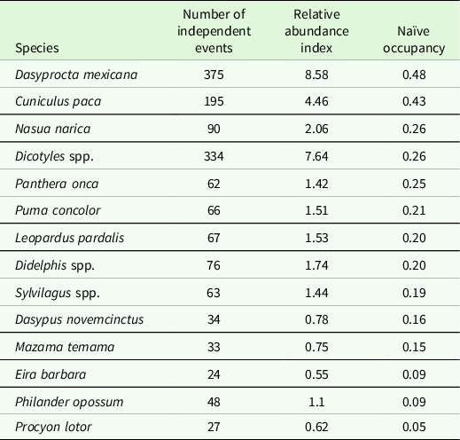
With a sampling effort of 4,373 camera days, the camera traps recorded 25,783 photographs and videos, of which 1,719 were independent events of 26 medium- and large-sized mammals. Of the total, 1,494 independent events corresponded to 14 predator and prey species under study (Table 1).
Table 1. Relative abundance index and naïve occupancy of predators and prey in the Chinantla region, southern Mexico.
As we studied 14 species, all the potential associations could be 14×13; that is, each species could be associated with the other 13, which gives us 182 possible associations. Not all the associations were found in the observed data, only 139 (prey-prey, prey-predator, and predator-predator). With the 10 executions of the bootstrap model, we found 77 constant co-occurrences. With respect to the procedure sensibility, for any 2 of the 10 executions, we have that at most d_1(F,G)=0.016, which indicates that at least the 98.4 % of the result of one execution has the same co-occurrences as the other execution, and non-co-occurrences bootstrapped, which indicates consistency in the executions. For the space-time co-occurrence network, we used 20 co-occurrences that corresponded to prey-predator and predator-predator (Fig. 2).
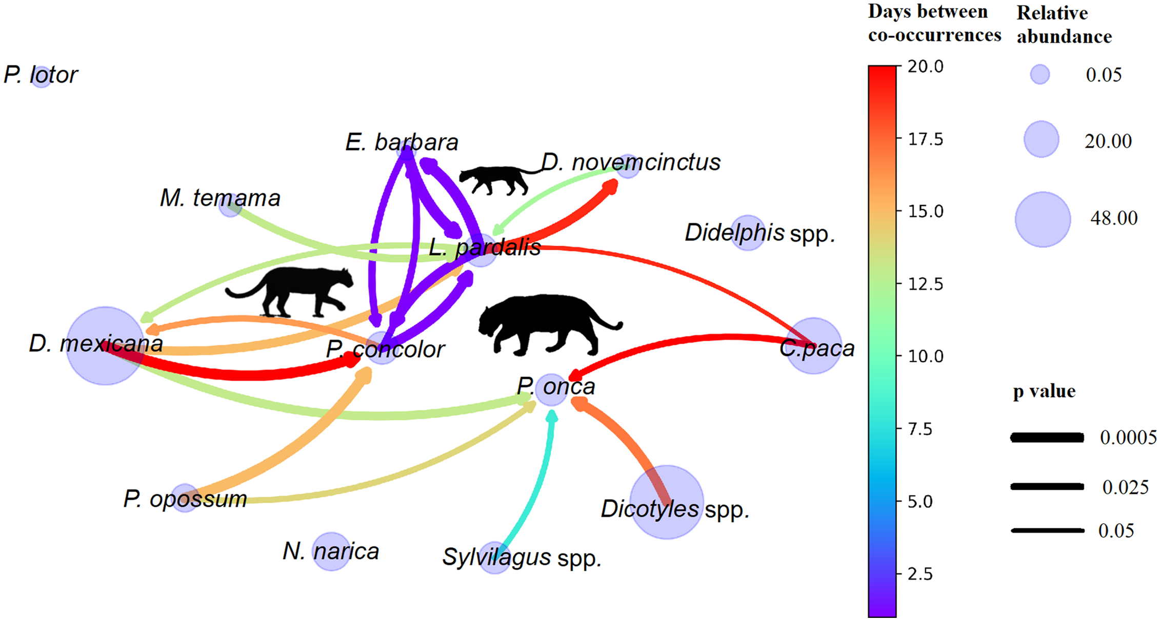
Figure 2. Ecological network of co-occurrences of predators and prey in the Chinantla region, southern Mexico. Only significant co-occurrences are shown (p < 0.05). The size of the circle indicates the relative abundance index value (RAI). The direction of the arrow indicates the species that occurs first (arrowhead) and the species that occurs later (arrow tail). The colour of the arrow indicates the day of lag in which one species passed and then another and corresponds to the legend on the right. The thickness of the arrow indicates the average p-value of the co-occurrence in the 10 executions, a thicker arrow implies a smaller average p-value.
The network allows us to see which species pass after another, the head of the arrow is the one that passes first, and how many days later, the colour of the arrow. In this way, we observe that prey are co-occurring several days after predators and that predators are generally not co-occurring with prey (absence of arrows directed from predators to prey). Predators co-occur with 8 of the 11 possible prey; there are species that only co-occur with one predator, but there are also some predators that share prey. Panthera onca co-occurred with five possible prey, two of which were exclusive: Dicotyles spp. and Silvylagus spp., whereas three species were shared: C. paca with L. pardalis, P. opossum with P. concolor, and D. mexicana with both P. concolor and L. pardalis. Puma concolor co-occurred with two prey species: D. mexicana and P. opossum, both were shared with P. onca. Leopardus pardalis co-occurred with four prey species, two were exclusive: M. temama and D. novemcinctus and two were shared: D. mexicana with both larger felids P. concolor and P. onca, and C. paca only with P. onca. Of the 11 potential prey species, three are not co-occurring with any predator neither in space nor time: N. narica, Didelphis spp., and P. lotor.
The spatiotemporal co-occurrence network shows that predators are generally not following prey, but apparently prey are displaying an avoidance behaviour. Panthera onca was the predator that co-occurred with the higher number of most potential prey, five potential prey passed after him in the same place: Dicotyles spp. co-occurred 16 days after (p = 0.00914), Sylvilagus spp. 7 days (p = 0.02849), C. paca, 14 days (p = 0.03926), D. mexicana, 12 days (p = 0.01809), and P. opossum, 13 days (p = 0.01928). With respect to P. concolor, four species co-occurred in space and time with this felid, two potential prey species: D. mexicana co-occurred after 19 days (p = 0.009) and P. opossum after 14 days (p = 0.010), whereas two carnivore species were observed the same day in the same sites (E. barbara, p = 0.024 and L. pardalis, p = 0.014) (Fig 2.).
For the third-largest felid, L. pardalis, four species was observed several days after: D. novemcinctus co-occurred after 11 days (p = 0.032), M. temama, 12 days (p = 0.022), D. mexicana, 14 days (p = 0.017), and C. paca, 18 days (p = 0.035). On the other hand, L. pardalis was found at the same site several days after two preys occurred: D. mexicana, 12 days (p = 0.029), and D. novemcinctus, 18 days (p = 0.016). Also, for L. pardalis we found a near coexistence with E. barbara and P. concolor, which co-occur in the same day (E. barbara, p = 0.009, and P. concolor, p = 0.024). Noticeably, we found L. pardalis and P. concolor co-occur on the same day (p = 0.014). Regarding large predator co-occurrences, we did not find that P. concolor and P. onca co-occur (Fig 2.)
Overlapping daily activity patterns
The overlaps between P. onca and its prey were overall moderate, with values ranging from Δ = 0.40 with N. narica to Δ = 0.75 with Sylvilagus spp. On the other hand, P. concolor presented overlap values Δ > 0.7 with C. paca, and Sylvilagus spp. Leopardus pardalis showed the highest overlap with C. paca (Δ = 0.81), Sylvilagus spp. (Δ = 0.78), Didelphis spp. (Δ = 0.73), and D. novemcinctus (Δ = 0.69; Table 2; Fig. S2). The highest daily temporal overlap was found between the predators: P. concolor and L. pardalis (Δ = 0.82) and P. onca and P. concolor (Δ = 0.81), while between P. onca and L. pardalis it was Δ = 0.77 (Table 2; Fig. S3).
Table 2. Daily temporal overlaps between predators and prey in the Chinantla region, southern Mexico. Delta value and 95% confidence intervals in parentheses Super index indicate the delta estimator used (1 when smaller sample was < 70 and 4 when smaller sample was =>70).

Discussion
Spatiotemporal co-occurrence between predators and prey
In this study, we propose a complementary approach to understand species co-occurrences using camera-trap data. We used three-dimensional matrix, bootstraps, and ecological networks to identify spatiotemporal co-occurrences in the search and avoidance phase of the predator-prey system in a neotropical ecosystem.
According to the method, the co-occurrences are not the product of randomness. We found several cases where if a predator passes through a site, a prey does not pass through the same site soon but several days later (See Figure 2). Consequently, it is hypothesized that prey could be avoiding predators in the spatial and temporal dimensions, as a strategy to minimize the risk of predation (Gaynor et al. Reference Gaynor, Brown, Middleton, Power and Brashares2019). For instance, C. paca and Dicotyles spp. occurred in the same site 19 and 16 days after P. onca, respectively; D. mexicana occurred 19 days after P. concolor; and D. mexicana and C. paca, occurred 14 and 18 days after L. pardalis, respectively. These findings also can be explained from the ‘ecology of fear’ theory, which proposed that the risk of predation is perceived by the prey, and in response, the prey shows anti-predatory behaviours, occurring in these cases, many days after the passage of the predators (Brown Reference Brown and Choe2019, Clinchy et al. Reference Clinchy, Sheriff and Zanette2012).
Overall, in the network (See Figure 2), we did not have evidence of active following behaviour of the predators, since they were not recorded in the same stations where their prey passed, neither on the same day, nor on subsequent days as we predicted, except for the pairs P. concolor - D. mexicana, L. pardalis - D. mexicana, and L. pardalis - D. novemcinctus, for which predator occurrence was many days later (> 12 days). One explanation may be that predators hunt by opportunistic encounters instead of following a particular prey clue, as has been suggested before for predator-prey systems in the neotropical region (Cavalcanti Reference Cavalcanti2008, Emmons Reference Emmons1987, Romero-Muñoz et al. Reference Romero-Muñoz, Maffei, Cuéllar and Noss2010). Another non-exclusive explanation is that predators perform an intermittent foraging (Dias et al. Reference Dias, Massara, de Campos and Rodrigues2019), in which individuals implement a search for prey in two phases: 1) intensive search in several sites and 2) rapid movements among sites. In the intensive search phase, the predator visits particular sites where it is more likely to find prey and lead an attack (Bénichou et al. Reference Bénichou, Loverdo, Moreau and Voituriez2011, Murakami & Gunji Reference Murakami and Gunji2017). The movement phase is generally performed quickly, with a low probability of encounters, but it allows travelling long distances. If the predator performs this kind of foraging, the predator will forage for a short time in different areas within its territory and thus prevent the prey in these areas displayed migratory behaviours, so that the foraged areas will almost always have prey availability (Bischoff-Mattson and Mattson Reference Bischoff-Mattson and Mattson2009). Telemetry studies support a multiphasic movement in felids; there are large movements related to travelling for patrolling home range, and there are active modes possibly during the prey searching (Clemenza et al. Reference Clemenza, Rubin, Johnson, Botta and Boyce2009, Núñez & Miller Reference Núñez-Pérez, Miller, Reyna-Hurtado and Chapman2019, van de Kerk et al. Reference Van de Kerk, Onorato, Criffield, Bolker, Augustine, McKinley and Oli2015). However, other studies found predators are stalking in both movement kinds due to features landscape selection are similar (Blake & Gese, Reference Blake and Gese2016). Such movements can also be in function to the seasonality of resources (Allen et al. Reference Allen, Engeman and Leung2014, Carrillo et al. Reference Carrillo, Fuller and Saenz2009, Montalvo et al. Reference Montalvo, Fuller, Saénz-Bolaños, Cruz-Díaz, Hagnauer, Herrera and Carrillo2020). Felines seem to be opportunistic predators taking advantage of contextual features and resources in ecosystems they inhabit (Ironside et al. Reference Ironside, Mattson, Theimer, Jansen, Holton, Arundel, Peters, Sexton and Edwards2017). Our analytic approach was adequate to show that co-occurrences between predator and prey were not the product of randomness and that predators are conducting an opportunistic hunting strategy.
Mazama temama, N. narica, and Dicotyles spp. are among the main prey of the large felids (Aranda & Sánchez-Cordero Reference Aranda and Sánchez-Cordero1996, Ávila-Nájera et al. Reference Ávila-Nájera, Palomares, Chávez, Tigar and Mendoza2018, Cruz et al. Reference Cruz, Muylaert, Galetti and Pires2021, Gómez-Ortiz et al. Reference Gómez-Ortiz, Monroy-Vilchis and Mendoza-Martínez2015, Rueda et al. Reference Rueda, Mendoza, Martínez and Rosas-Rosas2013), which explain the spatiotemporal avoidance pattern of those species found in this study. Prey should be mediated foraging, rest, and reproductive activities with the risk of being predated; therefore, any clue of predator presence will produce a change in the behaviour and changes on the habitat use, avoiding risky zones (Laundre Reference Laundré2010, Sih Reference Sih, Barbosa and Castellanos2005).
The relationships between predators and prey in the network can be explained from various theories because each of the species has developed different behaviours to avoid predation. Although a search behaviour was not observed by predators, the network allowed us to see that one of the most abundant species (D. mexicana) is related to the three felines. It is possible that, according to the aggregate response hypothesis, predators are concentrating their energy in areas where there is a higher density of prey (Hassell Reference Hassell1966). With regard to M. temama, we consider that being one of the main prey of P. onca and P. concolor, its lack of co-occurrences with both predators, can be explained from the hypothesis of the direct effect mediated by traits or behaviour, which is when the predators influence the distribution of prey (Muhly et al. Reference Muhly, Semeniuk, Massolo, Hickman and Musiani2011) in such a way that this species is not occupying the same sites as predators to avoid being predated.
Our study revealed that the daily activity overlaps of the activity patterns of P. onca, P. concolor, and L. pardalis with their prey were low in the case of N. narica, moderate with M. temama, D. mexicana, and Dicotyles spp., and high with C. paca, D. novemcinctus and Sylvilagus spp. These contrasts in activity overlaps have been reported previously (Chinchilla Reference Chinchilla1997, de Oliveira & Pereira Reference de Oliveira and Pereira2014, Estrada-Hernández Reference Estrada-Hernández2008, Harmsen et al. Reference Harmsen, Foster, Silver, Ostro and Doncaster2009, Rabinowitz & Nottingham Reference Rabinowitz and Nottingham1986). According to optimal foraging theory, predators tend to choose prey with the minor effort but with the highest energy supply; if the prey is abundant, predators will focus on it, reducing their feeding spectrum (Stephens & Krebs Reference Stephens and Krebs2019). Prey C. paca, D. novemcinctus and Sylvilagus spp. are manoeuvrable prey, whereas larger species such N. narica and Dicotyles spp. impose a higher risk of injuries during predation for felines. In the case of P. onca and P. concolor, it has been suggested that the activity patterns are synchronized with those of their prey (Foster et al. Reference Foster, Sarmento, Sollmann, Torres, Acomo, Negroes, Fonseca and Silveira2013, Herrera et al. Reference Herrera, Chávez, Alfaro, Fuller, Montalvo, Rodrigues and Carrillo2018); however, asynchronization has also been observed in studies with camera traps (Romero-Muñoz et al. Reference Romero-Muñoz, Maffei, Cuéllar and Noss2010). For these two large predators whose diet is versatile, an asynchronization with a greater number of prey species seems to be a better hunting strategy than synchronization with a single species (Romero-Muñoz et al. Reference Romero-Muñoz, Maffei, Cuéllar and Noss2010). In the case of the two main prey of the medium-sized predator L. pardalis, we found an asynchronization with D. mexicana (Δ = 0.50) but synchronization with C. paca (Δ = 0.81). It has been observed that the agoutis, such as D. mexicana, concentrates its activity at times of low risk of predation, especially when there is more food availability (Suselbeek et al. Reference Suselbeek, Emsens, Hirsch, Kays, Rowcliffe, Zamora-Gutierrez and Jansen2014).
With the two approaches, diary temporal overlap and time intervals, we measured two distinct axes of the animal behaviours. Approaches are complementary, not exclusive, whereas the overlap index pooled diary data for the species throughout surveys, the time interval measures inspect on the times (days) between co-occurrences in sites to disentangling any combined effect. In the overlap index, two species can have a high temporal overlap (e.g. felids and C. paca) because circadian rhythms, trained by intrinsic and extrinsic factors, dominate in the activity behaviours. Such temporal overlap, however, does not mean that two species will be active at the same site or day, so measuring the time between them provides a better insight into patterns of avoidance and tracking in predator-prey systems.
When species share common resources, such as space, time, or food, a subordinate species tends to segregate in any of these dimensions to allow coexistence (Gause Reference Gause1932). Coexistence was found between L. pardalis and P. concolor, since they co-occurred in the same sites on the same day and had a high synchrony in their daily activity patterns. Then, the partition of the food niche of both species can explain the coexistence at the temporal and spatial scales found in this study. Moreno et al. (Reference Moreno, Kays and Samudio2006) suggest that L. pardalis and P. concolor fit the energetic model proposed by Carbone (Reference Carbone2002) which indicates that small predators (< 21.5 kg) predate prey smaller than 45 % of their mass, and large predators (> 21.5 kg) are capable of consuming prey greater than 45 % of their mass. Consequently, P. concolor and L. pardalis are exploiting the same sites on the same times in search of prey of different size classes: P. concolor for large prey and L. pardalis for small prey (Sunquist & Sunquist Reference Sunquist and Sunquist2002). Future studies of the feeding habits of these species in the region will be able to complete the panorama of coexistence between both felids. A review of studies of activity patterns among the two species in Central and South America reported overlaps between 0.61 and 0.73, suggesting that these species overlap in their activity behaviours (Santos et al. Reference Santos, Carbone, Wearn, Rowcliffe, Espinosa, Moreira, Ahumada, Sousa, Trevelin, Alvarez-Loayza, Spironello, Jansen, Juen and Peres2019). In contrast, studies of feeding habits of these two species show a low (Chinchilla Reference Chinchilla1997, Gómez-Ortiz et al. Reference Gómez-Ortiz, Monroy-Vilchis and Mendoza-Martínez2015, Martins et al. Reference Martins, Quadros and Mazzolli2008) or moderate overlap in the prey they consume (Giordano et al. Reference Giordano, Lyra-Jorge, Miotto and Pivello2018, Moreno et al. Reference Moreno, Kays and Samudio2006), and rarely high overlap, probably as a consequence of the habitat condition (Tirelli et al. Reference Tirelli, de Freitas, Michalski, Percequillo and Eizirik2019).
Although we found a high overlap in the diary activity patterns between P. onca and P. concolor, co-occurrence analyses showed avoidance, which was similar to findings in others neotropical forest, where authors suggest such overlap is mediated by a spatial segregation (Foster et al. Reference Foster, Sarmento, Sollmann, Torres, Acomo, Negroes, Fonseca and Silveira2013, Harmsen et al. Reference Harmsen, Foster, Silver, Ostro and Doncaster2009). In this regard, it has been pointed out that P. onca temporarily or spatially displaces P. concolor (in 60% of 25 studies reviewed by Elbroch & Kusler Reference Elbroch and Kusler2018). However, in eight neotropical forests of South America, it was found that P. onca does not influence the habitat use of P. concolor, and although they presented a moderate or high temporal overlap, the activity peaks of P. concolor seem to avoid the hours of highest activity of P. onca (Santos et al. Reference Santos, Carbone, Wearn, Rowcliffe, Espinosa, Moreira, Ahumada, Sousa, Trevelin, Alvarez-Loayza, Spironello, Jansen, Juen and Peres2019). In this regard, we found puma activity peaks were displaced from the jaguar activity peak, being most evident at dawn, when the jaguar was inactive. Our results provide evidence of temporal and spatial avoidance of P. concolor to P. onca.
A surprising finding was to find the pairs of carnivores L. pardalis - E. barbara, and P. concolor - E. barbara, co-occurring on the same day in the same sites. The co-occurrence of these pairs was cyclical; that is, the passage of one species was followed by the passage of the other. The spatial coexistence observed among the felines and the mustelid is explained by the low overlap in the pattern of daily activity that occurred between them, while the felines were mainly nocturnal, the mustelid was mainly diurnal. A similar pattern of coexistence between L. pardalis and E. barbara was found by Massara et al. (Reference Massara, Paschoal, Bailey, Doherty, Barreto and Chiarello2018) in the Atlantic forest, where L. pardalis did not influence the spatial distribution of E. barbara. However, de Oliveira & Pereira (Reference de Oliveira and Pereira2014) found that P. concolor and L. pardalis exert a strong impact on the assembly of small carnivores, among which are E. barbara, that has been reported in the diet of these felines; temporal segregation reduces the probability of encounters and possible predation.
Our approach analyses the time intervals between species to measure the occurrence of one species and another at the same site in a different way than previous studies (Karanth et al. Reference Karanth, Srivathsa, Vasudev, Puri, Parameshwaran and Kumar2017, Parsons et al. Reference Parsons, Bland, Forresterd, Baker-Whattonf, Schuttlera, McShead, Costello and Kays2016). In addition, an advantage of the method and ecological networks used here is that it is feasible to analyse the co-occurrence between more than two species; for example, to test whether the presence of species A followed by species B increases the probability of species C passage or avoidance; for example, if Dicotyles spp. followed by P. onca dissuade the pass of P. concolor or not. Such patterns give us a panoramic view of the behaviour of the coexistence mechanisms. Future studies on time intervals and ecological networks can be directed to accommodate imperfect detection and to distinguish patterns between habitats (Gorini et al. Reference Gorini, Linnell, May, Panzacchi, Boitani, Odden and Nilsen2012, Morueta-Holme et al. Reference Morueta-Holme, Blonder, Sandel, McGill, Peet, Ott, Violle, Enquist, Jørgensen and Svenning2016). Also, it is of interest the reduction of the time intervals, instead of using 1 day, as in this study, using intervals of for example 4, 8 or 12 hrs. to obtain a finer pattern in the predator and prey search and avoidance phases. However, this will strongly depend on the amount of data obtained per station.
Conclusions
We found prey did not co-occur in time and space with predators in the short time. The prey delayed occurring in the sites where predators passed, suggesting that the prey perceives cues left by predators, and, consequently, they avoided the risky sites. In a similar way, we found subordinate predators (L. pardalis and P. concolor) are avoiding the apex predator because they co-occur in the same site several days later. Conversely, subordinate predators showed spatiotemporal coexistence perhaps facilitated by dietary segregation. In addition, we observed intra-guild associations between E. barbara, L. pardalis, and P. concolor allowed by a diary temporal segregation. Temporal overlap analyses did not provide evidence of a high temporal synchronization between predator and prey, with exception C. paca, Didelphis spp., and Sylvilagus spp, with all predators (L. pardalis, P. concolor, and P. onca). Also, and contrary to our expectations, predators exhibited a higher overlap with each other, suggesting that large predators prefer to have a broad activity pattern along the day to increase the chances of coinciding with several species instead of only one or few species. In this study, we provide a complementary method to the current methods for inferring coexistence mechanisms between species, such as the occupancy models of two species (Sollmann Reference Sollmann2018, Sollmann et al. Reference Sollmann, Furtado, Hofer, Jácomo, Tôrres and Silveira2012). And, we open a new research line to inquire into the behaviour mechanisms developed by species to allow coexistence within the framework of the fear ecology.
Supplementary material
To view supplementary material for this article, please visit https://doi.org/10.1017/S0266467422000189
Acknowledgement
We thank J. R. Prisciliano-Vázquez and local monitors for their valuable assistance in the field. Authorities of the communities of Cerro Concha, Cerro Mirador, Cerro Tepezcuintle, Emiliano Zapata, Leyes de Reforma, Luis Echeverría, Monte Negro, Nopalera del Rosario, Paso de San Jacobo, Paso Nuevo La Hamaca, Rancho Faisán, San Antonio del Barrio, San Cristóbal La Vega, San Mateo Yetla, San Rafael Agua Pescadito, Santa Cruz Tepetotutla, Soledad Vista Hermosa, and Vega de Sol.
Financial support
This work was supported by the Species Conservation Program of the National Commission of Natural Protected Areas (grant number PROCODES Chinantla 2011, 2012, 2013, 2014); Conservation Program for Sustainable Development; Secretaría de Investigación y Posgrado at the Instituto Politécnico Nacional (M.C.L., grant number SIP 20200286); and Mexican National Commission of Science and Technology (E.G.A., grant number 285671).
Conflicts of interests
The author(s) declare none.
Ethical statement
None.


