


1 Introduction
Flows around bluff bodies mounted on a flat plate appear in various technical applications, such as, e.g., turbomachinery blade flows or aircraft wing–body flows. We are interested in cylinder–wall junction flows because of their enormous importance in scour development around bridge piers in sandy river beds. The mechanism of scour development and its dependence on the flow field upstream of a pier was described many years ago (Melville & Raudkivi Reference Melville and Raudkivi1977). A major role has been attributed to the horseshoe vortex forming in front of a bridge pier. Such a horseshoe vortex has been observed in many different configurations of protuberances embedded in boundary layer flows. Due to the broad relevance of the horseshoe vortex for technical applications as well as for the fundamental understanding of flow physics, it is not surprising that in recent years a vast number of investigations addressing wall–body junction flows have been published – not only from the viewpoint of scour development but also concerning the flow field alone. We concentrate on findings addressing the dynamics of flows around long slender bodies such as cylinders, wings or bars, mounted perpendicularly on a flat plate. Many features occurring in such flows seem to be independent of the detailed structure of the fore-body (Escauriaza & Sotiropoulos Reference Escauriaza and Sotiropoulos2011; Schanderl & Manhart Reference Schanderl and Manhart2016).
If a boundary layer flow approaches a bluff body, the shear in the boundary layer gives rise to a vertical pressure gradient along the front of the body, driving the flow downwards to the wall. This downwash is deflected by the bottom wall and forms a spanwise vortex system (Devenport & Simpson Reference Devenport and Simpson1990). Parts of the downwash that become deflected by the bottom wall in front of the bluff body wrap up into a ellipsoidal main vortex V1. Other parts of the downwash feed an upstream-directed jet along the bottom wall underneath V1. After passing V1, the jet penetrates under the oncoming boundary layer and forms an extended recirculation zone. This eventually can wrap up into a second vortex V2 (Apsilidis et al. Reference Apsilidis, Diplas, Dancey and Bouratsis2015), which was not mentioned by Devenport & Simpson (Reference Devenport and Simpson1990), maybe due to a lack of resolution. Along the flow facing wall of the bluff body, the downwash establishes a boundary layer. Before reaching the bottom plate, this boundary layer has to separate from the body wall for the same reasons as the main flow separates from the bottom wall when approaching the bluff body. This separation leads to a third vortex V3 directly at the wall–cylinder junction rotating in the opposite direction to V1.
Due to the fact that the flow needs to bypass the protuberance, strong stretching in the spanwise direction occurs, increasing the spanwise vorticity of the vortex system and especially reinforcing the main vortex to an intense vortex, which is stretched around the body. Because their vortex axes are bent around the obstacle, such vortex systems are denoted as horseshoe vortices and associated with large wall stresses in the zone between the vortex and the body (Dargahi Reference Dargahi1989; Devenport & Simpson Reference Devenport and Simpson1990).
However, the discussion on the described flow topology is not complete. Apsilidis et al. (Reference Apsilidis, Diplas, Dancey and Bouratsis2015) suggested the possibility that vortex V2 is not a coherent flow structure but the time-averaged representation of a train of various small vortices. In accordance with Dargahi (Reference Dargahi1989), Escauriaza & Sotiropoulos (Reference Escauriaza and Sotiropoulos2011) observed two main vortices instead of only one. Furthermore, Escauriaza & Sotiropoulos (Reference Escauriaza and Sotiropoulos2011) stated that the number of vortices decreases with increasing Reynolds number, as long as the Reynolds number is within the investigated moderate range. On the contrary, Apsilidis et al. (Reference Apsilidis, Diplas, Dancey and Bouratsis2015) observed the time-averaged flow topology to be mainly invariant with the body Reynolds number (Apsilidis et al. Reference Apsilidis, Diplas, Dancey and Bouratsis2015) for moderate Reynolds numbers.
In addition to the topology of the time-averaged flow, in instantaneous flow fields, a variety of complicated phenomena have been observed. Devenport & Simpson (Reference Devenport and Simpson1990) described the wall jet underneath the horseshoe vortex as flipping between two modes: in the back-flow mode, the wall jet – having large upstream momentum – penetrates far into the oncoming boundary layer; in the zero-flow mode, the wall jet separates from the bottom wall relatively early and the fluid is ejected vertically away from the wall. In the zero-flow mode, V1 takes up a position further downstream than in the back-flow mode. Devenport & Simpson (Reference Devenport and Simpson1990) proposed that instantaneous structures in the incoming flow trigger the flipping between the two modes. Large-momentum fluid from the outer flow entering the vortex system might cause the back-flow mode, while fluid containing less momentum results in the zero-flow mode. However, they were not able to prove this hypothesis. Paik, Escauriaza & Sotiropoulos (Reference Paik, Escauriaza and Sotiropoulos2007) associated the back-flow mode with a well-organized vortex system, which undergoes instabilities due to its vicinity to the bottom wall. They descriptively discussed how hairpin vortices wrap around the main vortex, causing it to collapse and to be pushed towards the bluff body. They associated the resulting less organized vortex structure with the zero-flow mode.
Apsilidis et al. (Reference Apsilidis, Diplas, Dancey and Bouratsis2015) proposed that a third mode is present for a significant fraction of the time, the so-called intermediate mode, which bears none of the features associated with the back-flow and zero-flow modes. In this mode, the wall jet neither penetrates far into the oncoming flow nor is ejected vertically, but is diffused when running into the approaching boundary layer. The intermediate mode becomes more dominant with increasing Reynolds number (Apsilidis et al. Reference Apsilidis, Diplas, Dancey and Bouratsis2015). They furthermore stated that the position of the main vortex does not depend on the flow mode, as instantaneous flow topologies can be observed, in which V1 is located close to the cylinder even though the wall jet is in the back-flow mode. In addition, Apsilidis et al. (Reference Apsilidis, Diplas, Dancey and Bouratsis2015) observed that for a considerable fraction of the time, the flow topology cannot be associated with any of the modes due to a lack of visible coherent structures. With increasing Reynolds number, this fraction of time is decreasing.
The rich dynamics of the flow results in a typical distribution of turbulent kinetic energy. Devenport & Simpson (Reference Devenport and Simpson1990) observed large Reynolds stresses in the streamwise direction underneath the main vortex V1 close to the bottom plate and large Reynolds normal stresses in the vertical direction in the region covered by V1. Addition of both components of the Reynolds normal stresses leads to a vertical c-shaped pattern of turbulent kinetic energy
 $k$
(Paik et al.
Reference Paik, Escauriaza and Sotiropoulos2007). This distinct c-shape was confirmed and discussed in detail by Apsilidis et al. (Reference Apsilidis, Diplas, Dancey and Bouratsis2015), who studied the distribution of
$k$
(Paik et al.
Reference Paik, Escauriaza and Sotiropoulos2007). This distinct c-shape was confirmed and discussed in detail by Apsilidis et al. (Reference Apsilidis, Diplas, Dancey and Bouratsis2015), who studied the distribution of
 $k$
as well as of its in-plane contributors for a range of moderate Reynolds numbers. They found that the turbulent kinetic energy in the second patch of high turbulent kinetic energy, which forms the lower branch of the c-shape, increases with Reynolds number, while there is no clear trend for the amplitude of the turbulent kinetic energy in the upper branch around the vortex core.
$k$
as well as of its in-plane contributors for a range of moderate Reynolds numbers. They found that the turbulent kinetic energy in the second patch of high turbulent kinetic energy, which forms the lower branch of the c-shape, increases with Reynolds number, while there is no clear trend for the amplitude of the turbulent kinetic energy in the upper branch around the vortex core.
While the basic distribution of turbulent kinetic energy as observed by Devenport & Simpson (Reference Devenport and Simpson1990) in front of a wall-mounted bluff body has been confirmed by several research groups (Escauriaza & Sotiropoulos Reference Escauriaza and Sotiropoulos2011; Kirkil & Constantinescu Reference Kirkil and Constantinescu2015; Ryu et al. Reference Ryu, Emory, Iaccarino, Campos and Duraisamy2016; Schanderl & Manhart Reference Schanderl and Manhart2016), the discussion on the detailed mechanism causing such a shape is still ongoing. Devenport & Simpson (Reference Devenport and Simpson1990) proposed that the flipping of the main vortex V1 in the streamwise direction leads to large Reynolds normal stresses in the vertical as well as the streamwise direction in the region covered by V1. They furthermore suggested that the fluctuation behaviour of the wall jet causes the large Reynolds normal stresses in the lower branch of the c-shape: the amplitude of the streamwise velocity component is large in the back-flow mode here, while it is close to zero in the zero-flow mode. In contrast, Escauriaza & Sotiropoulos (Reference Escauriaza and Sotiropoulos2011), who observed two main vortices in the time-averaged flow topology, hypothesized a complex interaction of these two separated vortices and attributed the large amplitudes of the turbulent kinetic energy in the upper branch of the c-shape to the quasi-periodic merging, collapsing and regeneration of these vortices.
Our contribution to this ongoing discussion is the evaluation of the turbulence structure in front of a wall-mounted cylinder. The corresponding set-up is described in § 2. To gain a holistic set of data, we conducted both particle image velocimetry (§ 3) and large-eddy simulation (LES) (§ 4). Based on the time-averaged flow topology (§ 5) and its bimodality, we discuss the distribution of the turbulent kinetic energy as well as every single term of the budget of the turbulent kinetic energy, including production, convection, turbulent transport processes and dissipation (§ 6). We particularly intend to elucidate how these budget terms are linked to features of the time-averaged flow field, especially to acceleration and deceleration regions, and how they interact with each other.
2 Flow configuration
We investigate the flow around a cylinder placed vertically on the bottom wall in a water channel with a free surface at a low Froude number. The configuration is sketched in figure 1. The diameter of the cylinder is denoted as
 $D$
, the water depth is
$D$
, the water depth is
 $h=1.5D$
and the width of the channel is
$h=1.5D$
and the width of the channel is
 $w=11.7D$
. The approaching stream is a fully developed open-channel flow at a small Froude number (in fact, the Froude number is infinitesimal in the numerical simulation while it is
$w=11.7D$
. The approaching stream is a fully developed open-channel flow at a small Froude number (in fact, the Froude number is infinitesimal in the numerical simulation while it is
 $Fr=0.32$
in the experiment; see §§ 4 and 3 respectively). We devoted special care to the generation of a fully developed inflow, including the secondary flow structures in the channel (Nezu & Nakagawa Reference Nezu and Nakagawa1993). Based on the bulk velocity averaged over the whole cross-section of the channel,
$Fr=0.32$
in the experiment; see §§ 4 and 3 respectively). We devoted special care to the generation of a fully developed inflow, including the secondary flow structures in the channel (Nezu & Nakagawa Reference Nezu and Nakagawa1993). Based on the bulk velocity averaged over the whole cross-section of the channel,
 $u_{CS}$
, the Reynolds number is
$u_{CS}$
, the Reynolds number is
 $Re_{D}=u_{CS}D/\unicode[STIX]{x1D708}=39\,000$
in the LES and
$Re_{D}=u_{CS}D/\unicode[STIX]{x1D708}=39\,000$
in the LES and
 $Re_{D}=u_{CS}D/\unicode[STIX]{x1D708}=37\,165\pm 7\,\%$
in the experiment. The uncertainty in the experiment is due to uncertainties in the flow rate, flow depth and temperature of the working fluid. Due to the secondary flow developing in the channel, the global bulk velocity
$Re_{D}=u_{CS}D/\unicode[STIX]{x1D708}=37\,165\pm 7\,\%$
in the experiment. The uncertainty in the experiment is due to uncertainties in the flow rate, flow depth and temperature of the working fluid. Due to the secondary flow developing in the channel, the global bulk velocity
 $u_{CS}$
differs from the bulk velocity in the symmetry plane
$u_{CS}$
differs from the bulk velocity in the symmetry plane
 $u_{b}$
, such that
$u_{b}$
, such that
 $u_{b}=1.075u_{CS}$
in the LES and
$u_{b}=1.075u_{CS}$
in the LES and
 $u_{b}=1.031u_{CS}$
in the experiment; the corresponding Reynolds numbers are accordingly
$u_{b}=1.031u_{CS}$
in the experiment; the corresponding Reynolds numbers are accordingly
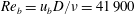 $Re_{b}=u_{b}D/\unicode[STIX]{x1D708}=41\,900$
in the LES and
$Re_{b}=u_{b}D/\unicode[STIX]{x1D708}=41\,900$
in the LES and
 $Re_{b}=u_{b}D/\unicode[STIX]{x1D708}=38\,300$
in the experiment. We use the bulk velocity of the symmetry plane for normalization in the remainder of this paper, as this allows a better comparison with results from the literature for the quantities in the symmetry plane.
$Re_{b}=u_{b}D/\unicode[STIX]{x1D708}=38\,300$
in the experiment. We use the bulk velocity of the symmetry plane for normalization in the remainder of this paper, as this allows a better comparison with results from the literature for the quantities in the symmetry plane.

Figure 1. The configuration of the flow around a wall-mounted cylinder at
 $Re_{D}=39\,000$
.
$Re_{D}=39\,000$
.
The parameters of the configuration have been chosen to be comparable to the experiments of Dargahi (Reference Dargahi1989) and preliminary studies of our research group (Pfleger Reference Pfleger2011). The results of Dargahi (Reference Dargahi1989) have frequently been used for validating numerical results (Roulund et al. Reference Roulund, Sumer, Fredsoe and Michelsen2005; Escauriaza & Sotiropoulos Reference Escauriaza and Sotiropoulos2011). The configuration of the experiment of Apsilidis et al. (Reference Apsilidis, Diplas, Dancey and Bouratsis2015) differs from ours in the ratio of the cylinder diameter to the boundary layer thickness and in the ratio of the water depth to the channel width. However, it was performed at a similar Reynolds number. Furthermore, Devenport & Simpson (Reference Devenport and Simpson1990) investigated a wing–body junction flow at a larger Reynolds number and a smaller boundary layer thickness-to-diameter ratio than ours. Nevertheless, many flow features are shared among the cited comparable studies.
3 Experimental configuration
We conducted particle image velocimetry (PIV) experiments in the hydromechanics laboratory of the Technische Universität München. First, the experimental set-up is described. Subsequently, the measuring technique and the post-processing parameters are briefly introduced.
3.1 Experimental domain
The water channel is sketched in figure 2. A cylinder with a diameter of
 $D=0.1$
m is placed in the symmetry plane of a
$D=0.1$
m is placed in the symmetry plane of a
 $11.7D$
wide flume. The latter is fed by a high-level water tank. The flow rate is measured by a magneto-inductive flow meter. A flow straightener damps the flow disturbances introduced by the inlet and a floating body reduces surface waves at the beginning of the channel. The undisturbed section of the flume in which the approaching turbulent open-channel flow develops naturally is approximately
$11.7D$
wide flume. The latter is fed by a high-level water tank. The flow rate is measured by a magneto-inductive flow meter. A flow straightener damps the flow disturbances introduced by the inlet and a floating body reduces surface waves at the beginning of the channel. The undisturbed section of the flume in which the approaching turbulent open-channel flow develops naturally is approximately
 $200D$
long. A sluice placed at the outlet of the flume controls the flow depth to
$200D$
long. A sluice placed at the outlet of the flume controls the flow depth to
 $1.5D$
before the water recirculates to the inlet periodically. The temperature of the working fluid water was found to be essentially constant at
$1.5D$
before the water recirculates to the inlet periodically. The temperature of the working fluid water was found to be essentially constant at
 $18.4\,^{\circ }\text{C}$
, which gives a kinematic viscosity of
$18.4\,^{\circ }\text{C}$
, which gives a kinematic viscosity of
 $1.05\times 10^{-6}~\text{m}^{2}~\text{s}^{-1}$
.
$1.05\times 10^{-6}~\text{m}^{2}~\text{s}^{-1}$
.

Figure 2. Experimental set-up, taken from Pfleger (Reference Pfleger2011).
Since the cylinder disturbs the flow, small-scale surface waves appear and change the angle of refraction locally. Therefore, we used a slat of acrylic glass to damp those impacts to enable the laser light to enter the water body perpendicularly at its surface. The slat was designed to be just as large as necessary to keep the influence on the flow structure as small as possible. It had a length of
 $L=1.5D$
in the streamwise direction, a width of
$L=1.5D$
in the streamwise direction, a width of
 $W=0.5D$
in the spanwise direction and was submerged by
$W=0.5D$
in the spanwise direction and was submerged by
 $0.01D$
–
$0.01D$
–
 $0.05D$
. Approximately 4 % of the flume width was covered by the slat. In order to study its influence, the approaching flow with and without the slat was measured. In addition, numerical simulations of the flow around the cylinder with and without such a slat at lower Reynolds numbers were executed. The comparison of both numerical simulation and measurement of the approaching flow indicated that the deviations in the regions of interest near the bottom wall were small.
$0.05D$
. Approximately 4 % of the flume width was covered by the slat. In order to study its influence, the approaching flow with and without the slat was measured. In addition, numerical simulations of the flow around the cylinder with and without such a slat at lower Reynolds numbers were executed. The comparison of both numerical simulation and measurement of the approaching flow indicated that the deviations in the regions of interest near the bottom wall were small.
3.2 Measuring technique
We used two-dimensional two-component PIV to measure instantaneous velocity vectors in an observation window located in the symmetry plane upstream of the cylinder. A
 $2~\text{mm}=0.02D$
thick light sheet was generated by a 532 nm Nd : YAG laser and entered the flow from the top through the slat. The images were recorded with a CCD camera at a resolution of
$2~\text{mm}=0.02D$
thick light sheet was generated by a 532 nm Nd : YAG laser and entered the flow from the top through the slat. The images were recorded with a CCD camera at a resolution of
 $2048\times 2048~\text{px}$
. We applied two different magnifications for the inflow and the flow in front of the cylinder respectively. For the inflow, we covered the whole flow depth, which resulted in a resolution of
$2048\times 2048~\text{px}$
. We applied two different magnifications for the inflow and the flow in front of the cylinder respectively. For the inflow, we covered the whole flow depth, which resulted in a resolution of
 $87~\unicode[STIX]{x03BC}\text{m}~\text{px}^{-1}$
. For the measurements in front of the cylinder, we zoomed in using an
$87~\unicode[STIX]{x03BC}\text{m}~\text{px}^{-1}$
. For the measurements in front of the cylinder, we zoomed in using an
 $f$
-number and a focal length of 2.8 and 105 mm respectively. Thereby, we achieved a magnification factor of 0.155, i.e.
$f$
-number and a focal length of 2.8 and 105 mm respectively. Thereby, we achieved a magnification factor of 0.155, i.e.
 $47.6~\unicode[STIX]{x03BC}\text{m}~\text{px}^{-1}$
or
$47.6~\unicode[STIX]{x03BC}\text{m}~\text{px}^{-1}$
or
 $2101~\text{px}/D$
.
$2101~\text{px}/D$
.
The seeding particles were hollow glass spheres with a diameter of
 $d_{P}=10~\unicode[STIX]{x03BC}\text{m}$
and a density of
$d_{P}=10~\unicode[STIX]{x03BC}\text{m}$
and a density of
 $\unicode[STIX]{x1D70C}_{P}=1100~\text{kg}~\text{m}^{-3}$
. The corresponding relaxation time was thus
$\unicode[STIX]{x1D70C}_{P}=1100~\text{kg}~\text{m}^{-3}$
. The corresponding relaxation time was thus
 $\unicode[STIX]{x1D70F}_{P}=d_{P}^{2}\unicode[STIX]{x1D70C}_{P}/(18\unicode[STIX]{x1D708}\unicode[STIX]{x1D70C})=6.11\times 10^{-6}~\text{s}$
(Raffel et al.
Reference Raffel, Willert, Wereley and Kompenhans2007). With this relaxation time, we could evaluate different Stokes numbers. The Stokes number based on the outer scaling was
$\unicode[STIX]{x1D70F}_{P}=d_{P}^{2}\unicode[STIX]{x1D70C}_{P}/(18\unicode[STIX]{x1D708}\unicode[STIX]{x1D70C})=6.11\times 10^{-6}~\text{s}$
(Raffel et al.
Reference Raffel, Willert, Wereley and Kompenhans2007). With this relaxation time, we could evaluate different Stokes numbers. The Stokes number based on the outer scaling was
 $St_{b}=\unicode[STIX]{x1D70F}_{P}u_{b}/D=2.38\times 10^{-5}$
. Applying the Kolmogorov time scale
$St_{b}=\unicode[STIX]{x1D70F}_{P}u_{b}/D=2.38\times 10^{-5}$
. Applying the Kolmogorov time scale
 $\unicode[STIX]{x1D70F}_{K}=\sqrt{\unicode[STIX]{x1D708}/\unicode[STIX]{x1D716}_{macro}}$
(Pope Reference Pope2011), the corresponding Stokes number was
$\unicode[STIX]{x1D70F}_{K}=\sqrt{\unicode[STIX]{x1D708}/\unicode[STIX]{x1D716}_{macro}}$
(Pope Reference Pope2011), the corresponding Stokes number was
 $St_{K}=\unicode[STIX]{x1D70F}_{P}/\unicode[STIX]{x1D70F}_{K}=4.7145\times 10^{-3}$
. The macroscale estimation of the dissipation,
$St_{K}=\unicode[STIX]{x1D70F}_{P}/\unicode[STIX]{x1D70F}_{K}=4.7145\times 10^{-3}$
. The macroscale estimation of the dissipation,
 $\unicode[STIX]{x1D716}_{macro}=u_{b}^{3}/D$
(Pope Reference Pope2011), is a conservative estimation, as the discussion of the dissipation in § 6.4 will show. Since the estimated Stokes numbers are considerably smaller than one, the particles can be considered to attain velocity equilibrium with the fluid (Raffel et al.
Reference Raffel, Willert, Wereley and Kompenhans2007). The seeding was given continuously to the flow at the flow straightener at the beginning of the flume (figure 2).
$\unicode[STIX]{x1D716}_{macro}=u_{b}^{3}/D$
(Pope Reference Pope2011), is a conservative estimation, as the discussion of the dissipation in § 6.4 will show. Since the estimated Stokes numbers are considerably smaller than one, the particles can be considered to attain velocity equilibrium with the fluid (Raffel et al.
Reference Raffel, Willert, Wereley and Kompenhans2007). The seeding was given continuously to the flow at the flow straightener at the beginning of the flume (figure 2).
We recorded a total of 27 000 image pairs with a sampling rate of 7.25 Hz and a time delay of
 $700~\unicode[STIX]{x03BC}\text{s}$
. This sampling rate would be too low to trace the evolution of individual flow structures in time or to compute spectra. For our purpose, it was sufficient as we considered time-averaged quantities only. Due to computer capacity, we subdivided the experiment into 18 batches of 1500 image pairs. This allowed us to clean the glass bottom of the flume repeatedly between each run to keep surface reflections at a constant low level. Thus, we recorded the flow statistics within a dimensionless time
$700~\unicode[STIX]{x03BC}\text{s}$
. This sampling rate would be too low to trace the evolution of individual flow structures in time or to compute spectra. For our purpose, it was sufficient as we considered time-averaged quantities only. Due to computer capacity, we subdivided the experiment into 18 batches of 1500 image pairs. This allowed us to clean the glass bottom of the flume repeatedly between each run to keep surface reflections at a constant low level. Thus, we recorded the flow statistics within a dimensionless time
 $Tu_{b}/D\approx 800$
in each batch and
$Tu_{b}/D\approx 800$
in each batch and
 $Tu_{b}/D\approx 15\,000$
in total.
$Tu_{b}/D\approx 15\,000$
in total.
To analyse the flow field, we applied a two-dimensional standard PIV vector evaluation with
 $16\times 16~\text{px}$
interrogation windows at a 50 % overlap. The vectors marked as invalid were replaced by their corresponding
$16\times 16~\text{px}$
interrogation windows at a 50 % overlap. The vectors marked as invalid were replaced by their corresponding
 $32\times 32$
interrogation window counterparts. Thus, the spatial resolution was
$32\times 32$
interrogation window counterparts. Thus, the spatial resolution was
 $0.0038D$
, which corresponds to 263 data points per cylinder diameter.
$0.0038D$
, which corresponds to 263 data points per cylinder diameter.
In order to validate our PIV results, we checked various evaluation algorithms. An interrogation window size of
 $32\times 32$
px was too coarse to resolve fine structures in the flow statistics. A standard evaluation with an interrogation window size of
$32\times 32$
px was too coarse to resolve fine structures in the flow statistics. A standard evaluation with an interrogation window size of
 $16\times 16$
px yielded a large number of invalid vectors. We explain these invalid vectors by out-of-plane losses due to large spanwise velocity fluctuations perpendicular to the light sheet. Unfortunately, the out-of-plane losses produced some artefacts in the flow fields. The artefacts disappeared when a deformable window algorithm was used. However, this algorithm marked an even larger number of samples as invalid. Therefore, we decided to use a standard
$16\times 16$
px yielded a large number of invalid vectors. We explain these invalid vectors by out-of-plane losses due to large spanwise velocity fluctuations perpendicular to the light sheet. Unfortunately, the out-of-plane losses produced some artefacts in the flow fields. The artefacts disappeared when a deformable window algorithm was used. However, this algorithm marked an even larger number of samples as invalid. Therefore, we decided to use a standard
 $16\times 16$
interrogation window evaluation and to replace the vectors marked as invalid by their counterparts from a
$16\times 16$
interrogation window evaluation and to replace the vectors marked as invalid by their counterparts from a
 $32\times 32$
interrogation window evaluation at the same spatial positions. The results obtained with this technique were very similar to the ones obtained by the
$32\times 32$
interrogation window evaluation at the same spatial positions. The results obtained with this technique were very similar to the ones obtained by the
 $16\times 16$
evaluation with window deformation, although some details were lost. We feel this to be a good compromise between resolution and reliability. In figure 3, the number of valid samples in the region of interest in front of the cylinder is plotted. In wide regions, more than 24 000 samples were achieved. The reduced number of samples near the corner between the cylinder and the wall (figure 3) corresponds to the region of the corner vortex in which there are both large spanwise fluctuations and large spatial velocity gradients.
$16\times 16$
evaluation with window deformation, although some details were lost. We feel this to be a good compromise between resolution and reliability. In figure 3, the number of valid samples in the region of interest in front of the cylinder is plotted. In wide regions, more than 24 000 samples were achieved. The reduced number of samples near the corner between the cylinder and the wall (figure 3) corresponds to the region of the corner vortex in which there are both large spanwise fluctuations and large spatial velocity gradients.

Figure 3. The number of valid samples obtained in the PIV experiment.
In addition to the standard interrogation window algorithm, we applied a single-pixel evaluation (Westerweel, Geelhoed & Lindken Reference Westerweel, Geelhoed and Lindken2004; Kähler, Scholz & Ortmanns Reference Kähler, Scholz and Ortmanns2006; Strobl, Jenssen & Manhart Reference Strobl, Jenssen and Manhart2016) to evaluate the time-averaged flow field. This gave a resolution of 2083 data points per diameter. Although these fields were quite noisy, they were useful for assessing the time-averaged wall shear stress and for revealing further details of the flow field.
To document the undisturbed approach flow, the cylinder was removed. The corresponding measurements were conducted at the same streamwise position in the symmetry plane of the channel as the ones with the cylinder. To capture the whole flow depth, they were conducted with a larger field of view. The evaluation was made with interrogation windows of
 $32\times 32~\text{px}$
, which corresponds to 72 data points per cylinder diameter. As this resolution was insufficient for an estimation of the wall gradient, the method of Clauser (Reference Clauser1954) was applied to estimate the undisturbed wall shear stress of the approach flow. This is justifiable since the approach flow is considered to be a fully developed open-channel flow. It should be noted that the wall shear stress in front of the cylinder was evaluated by computing the velocity gradient.
$32\times 32~\text{px}$
, which corresponds to 72 data points per cylinder diameter. As this resolution was insufficient for an estimation of the wall gradient, the method of Clauser (Reference Clauser1954) was applied to estimate the undisturbed wall shear stress of the approach flow. This is justifiable since the approach flow is considered to be a fully developed open-channel flow. It should be noted that the wall shear stress in front of the cylinder was evaluated by computing the velocity gradient.
4 Computational configuration
We complemented our PIV measurements by a highly resolved LES of the same flow configuration, identical to the one described in the study of Schanderl & Manhart (Reference Schanderl and Manhart2016), in which the reliability of the presented simulation has been discussed in detail. In this section, we describe the numerical method and set-up before we discuss the influence of the modelled subgrid-scale stresses on the results.
4.1 Numerical method
For the highly resolved LES, we applied our in-house code MGLET, which is a finite volume code and parametrizes the subgrid-scale stresses by the wall-adapting local eddy-viscosity (WALE) model (Nicoud & Ducros Reference Nicoud and Ducros1999). Since the subgrid-scale viscosity in this model decreases naturally towards the wall with
 $\unicode[STIX]{x1D708}_{t}\propto y^{3}$
, no damping function had to be used. Central differences and a third-order Runge–Kutta procedure provide spatial approximation and time integration respectively. Since the grid is Cartesian, a conservative second-order immersed boundary method (Peller et al.
Reference Peller, Duc, Tremblay and Manhart2006; Peller Reference Peller2010) is applied to constitute the curved surface of the cylinder. The variables are arranged in a staggered way. Zonally embedded grids (Manhart Reference Manhart2004), each reducing the grid spacing by a factor of two, refine the grid in the region of interest around the cylinder.
$\unicode[STIX]{x1D708}_{t}\propto y^{3}$
, no damping function had to be used. Central differences and a third-order Runge–Kutta procedure provide spatial approximation and time integration respectively. Since the grid is Cartesian, a conservative second-order immersed boundary method (Peller et al.
Reference Peller, Duc, Tremblay and Manhart2006; Peller Reference Peller2010) is applied to constitute the curved surface of the cylinder. The variables are arranged in a staggered way. Zonally embedded grids (Manhart Reference Manhart2004), each reducing the grid spacing by a factor of two, refine the grid in the region of interest around the cylinder.
To model the flow configuration in figure 1, the cylinder and the bottom and sidewalls of the channel are represented as no-slip conditions. The free surface is modelled by a slip condition. Since this slip condition at the top boundary prevents all kinds of surface deformation, the Froude number can be assumed to be infinitesimally small.
We assume that we have a wall-resolved LES, which means that we assess the local instantaneous wall shear stress by the linear gradient between the first off-wall grid cell centre and the wall. This assumption is justified if the wall-nearest cell centres are within the viscous sublayer, which is fulfilled in most of the flow domain, except in the precursor simulation; see below.
After the flow has reached a statistically steady state, a dimensionless time of
 $Tu_{b}/D\approx 700$
was simulated to gather statistics. This took approximately 2 million cpu hours on the high-performance computer SUPERMUC of the Bavarian Academy of Sciences.
$Tu_{b}/D\approx 700$
was simulated to gather statistics. This took approximately 2 million cpu hours on the high-performance computer SUPERMUC of the Bavarian Academy of Sciences.
4.2 Grid resolution
The computational domain consists of two major parts (figure 4): a precursor grid with periodic boundary conditions in the streamwise direction (
 $x$
-direction) simulating the fully developed open-channel flow and the base grid in which the cylinder is placed. The base grid is one-way coupled to the precursor grid, such that instantaneous velocity cross-sections are taken from the precursor and set as the inflow condition at the base grid. The cylinder is placed at
$x$
-direction) simulating the fully developed open-channel flow and the base grid in which the cylinder is placed. The base grid is one-way coupled to the precursor grid, such that instantaneous velocity cross-sections are taken from the precursor and set as the inflow condition at the base grid. The cylinder is placed at
 $(x,y)=(0,0)$
, which corresponds to the centre of the base grid.
$(x,y)=(0,0)$
, which corresponds to the centre of the base grid.
The region of interest around the cylinder is refined by locally embedded grids. In total, three levels of grid refinement had to be applied. The precursor and base grid correspond to the refinement level zero and the finest grid to refinement level three. The position of each local grid is indicated by grey colour in figure 4. Since each refinement level reduces the grid spacing by a factor of two, the grid spacing of the finest level is eight times smaller than that in the precursor and the base grid. The finest grid uses 250 grid cells per cylinder diameter in the horizontal directions and 1000 grid cells per diameter in the vertical direction (
 $z$
-direction), normal to the bottom wall. This corresponds to
$z$
-direction), normal to the bottom wall. This corresponds to
 $\unicode[STIX]{x0394}x^{+}=\unicode[STIX]{x0394}y^{+}=7.4$
and
$\unicode[STIX]{x0394}x^{+}=\unicode[STIX]{x0394}y^{+}=7.4$
and
 $\unicode[STIX]{x0394}z^{+}=1.9$
in wall units based on the undisturbed wall shear stress
$\unicode[STIX]{x0394}z^{+}=1.9$
in wall units based on the undisturbed wall shear stress
 $\unicode[STIX]{x1D70F}_{0}$
of the flow in the precursor simulation.
$\unicode[STIX]{x1D70F}_{0}$
of the flow in the precursor simulation.
The wall-nearest grid point, which is in the cell centre of the wall-nearest grid cell, is at
 $z^{+}=7.5$
in the precursor simulation. In the finest grid around the cylinder, this is at
$z^{+}=7.5$
in the precursor simulation. In the finest grid around the cylinder, this is at
 $z^{+}=0.95$
if it is based on the wall shear stress of the oncoming flow. If the local wall shear stress is taken, the maximum inner wall distance of the first grid point in the symmetry plane lies at
$z^{+}=0.95$
if it is based on the wall shear stress of the oncoming flow. If the local wall shear stress is taken, the maximum inner wall distance of the first grid point in the symmetry plane lies at
 $z^{+}\approx 1.6$
.
$z^{+}\approx 1.6$
.
As the discussion of the dissipation rate in § 6.4 indicates, the finest grid spacing corresponds to approximately 1.5 Kolmogorov length scales in the vertical and approximately 6 Kolmogorov length scales in the horizontal direction. A grid study (Schanderl & Manhart Reference Schanderl and Manhart2016) shows that the three refinement levels applied are sufficient to reach a converged solution of the flow. The convergence of the first-order moments of the flow field is exemplarily discussed in § 5.3, where the wall shear stress distributions of three single simulations with one, two and three levels of grid refinement are presented. All numerical data relating to the region around the cylinder presented in this paper are taken from the simulation with three levels of grid refinement. However, as no locally embedded grids are applied in the inflow section, data characterizing this incoming flow are taken from the grid corresponding to refinement level zero.
The grid is equidistant in the horizontal directions and stretched by a factor of less than 1.01 in the vertical direction. It should be noted that as this stretching factor is applied to the base grid, only every eighth cell of the finest local grid is stretched. In total, the simulation uses
 $400\times 10^{6}$
grid cells.
$400\times 10^{6}$
grid cells.
Application of time steps of
 $\unicode[STIX]{x0394}Tu_{b}/D=5.34\times 10^{-4}$
results in a Courant–Friedrichs–Lewy number of
$\unicode[STIX]{x0394}Tu_{b}/D=5.34\times 10^{-4}$
results in a Courant–Friedrichs–Lewy number of
 $0.55<CFL_{max}<0.82$
on the finest locally embedded grid in the region around the cylinder.
$0.55<CFL_{max}<0.82$
on the finest locally embedded grid in the region around the cylinder.

Figure 4. Side view of the computational domain. The zonally embedded grids are marked in grey (Schanderl & Manhart Reference Schanderl and Manhart2016).
4.3 Influence of the subgrid-scale model
The grid spacing is fine enough to ensure that the influence of the subgrid-scale model is small (Schanderl & Manhart Reference Schanderl and Manhart2016). Compared with the molecular viscosity
 $\unicode[STIX]{x1D708}$
, the time-averaged modelled viscosity does not exceed a value of
$\unicode[STIX]{x1D708}$
, the time-averaged modelled viscosity does not exceed a value of
 $\langle \unicode[STIX]{x1D708}_{t}\rangle =0.39\unicode[STIX]{x1D708}$
in the symmetry plane in front of the cylinder. Schanderl & Manhart (Reference Schanderl and Manhart2016) furthermore demonstrated that the time-averaged molecular shear stress
$\langle \unicode[STIX]{x1D708}_{t}\rangle =0.39\unicode[STIX]{x1D708}$
in the symmetry plane in front of the cylinder. Schanderl & Manhart (Reference Schanderl and Manhart2016) furthermore demonstrated that the time-averaged molecular shear stress
 $\unicode[STIX]{x1D708}\unicode[STIX]{x2202}\langle u\rangle /\unicode[STIX]{x2202}z$
and the resolved turbulent shear stress
$\unicode[STIX]{x1D708}\unicode[STIX]{x2202}\langle u\rangle /\unicode[STIX]{x2202}z$
and the resolved turbulent shear stress
 $-\unicode[STIX]{x1D70C}\langle u^{\prime }w^{\prime }\rangle$
exceed the modelled shear stress
$-\unicode[STIX]{x1D70C}\langle u^{\prime }w^{\prime }\rangle$
exceed the modelled shear stress
 $\langle \unicode[STIX]{x1D708}_{t}\unicode[STIX]{x2202}u/\unicode[STIX]{x2202}z\rangle$
by two orders of magnitude in the region of the horseshoe vortex system. Here,
$\langle \unicode[STIX]{x1D708}_{t}\unicode[STIX]{x2202}u/\unicode[STIX]{x2202}z\rangle$
by two orders of magnitude in the region of the horseshoe vortex system. Here,
 $u^{\prime }$
,
$u^{\prime }$
,
 $v^{\prime }$
and
$v^{\prime }$
and
 $w^{\prime }$
are the fluctuations of the corresponding velocities in the streamwise, spanwise and vertical directions
$w^{\prime }$
are the fluctuations of the corresponding velocities in the streamwise, spanwise and vertical directions
 $u$
,
$u$
,
 $v$
and
$v$
and
 $w$
respectively.
$w$
respectively.
Since the presented study focuses on the turbulent kinetic energy balance, we took care that the resolved turbulent kinetic energy
 $k$
,
$k$
,
 $$\begin{eqnarray}k={\textstyle \frac{1}{2}}(\langle u^{\prime 2}\rangle +\langle v^{\prime 2}\rangle +\langle w^{\prime 2}\rangle ),\end{eqnarray}$$
was large compared with the modelled turbulent kinetic energy
 $k_{SGS}$
, which is estimated by (Lilly Reference Lilly1967; Werner Reference Werner1991)
$k_{SGS}$
, which is estimated by (Lilly Reference Lilly1967; Werner Reference Werner1991)
 $$\begin{eqnarray}k_{SGS}=\left(\frac{\unicode[STIX]{x1D708}_{t}}{0.094\unicode[STIX]{x1D6E5}}\right)^{2}.\end{eqnarray}$$
Here,
 $\unicode[STIX]{x1D6E5}$
is the filter width, which is equivalent to the grid spacing.
$\unicode[STIX]{x1D6E5}$
is the filter width, which is equivalent to the grid spacing.
In figure 5, the ratio of the modelled to the resolved turbulent kinetic energy
 $k_{SGS}/k$
is evaluated in the symmetry plane in front of the cylinder in an area covered by the horseshoe vortex system. In the region around the horseshoe vortex centre, the modelled turbulent kinetic energy peaks at
$k_{SGS}/k$
is evaluated in the symmetry plane in front of the cylinder in an area covered by the horseshoe vortex system. In the region around the horseshoe vortex centre, the modelled turbulent kinetic energy peaks at
 $k_{SGS}\approx 0.035k$
.
$k_{SGS}\approx 0.035k$
.
At the junction of the bottom wall and the cylinder, values of
 $k_{SGS}/k\approx 0.15$
can be observed. Here, the subgrid stress model visibly contributes to the energy balance. The peak at this position implies that the grid is too coarse to fully resolve the turbulent kinetic energy of the small corner vortex (see § 5). This is visible in the residual of the turbulent kinetic energy budget discussed in § 6.6. However, for an LES, this magnitude of
$k_{SGS}/k\approx 0.15$
can be observed. Here, the subgrid stress model visibly contributes to the energy balance. The peak at this position implies that the grid is too coarse to fully resolve the turbulent kinetic energy of the small corner vortex (see § 5). This is visible in the residual of the turbulent kinetic energy budget discussed in § 6.6. However, for an LES, this magnitude of
 $k_{SGS}/k$
can be considered as small. Furthermore, the peak is locally restricted, while in large regions,
$k_{SGS}/k$
can be considered as small. Furthermore, the peak is locally restricted, while in large regions,
 $k_{SGS}/k$
is significantly smaller.
$k_{SGS}/k$
is significantly smaller.
Considering the small contribution of the subgrid stresses, we assume that the observations concerning the turbulent kinetic energy budget discussed in § 6 are representative for this flow, despite the fact that the presented data apart from the dissipation do not include subgrid contributions. As pointed out in § 6.4, the modelled dissipation is approximately
 $1/10$
to
$1/10$
to
 $1/3$
in the region covered by the horseshoe vortex. For the evaluation of the dissipation, therefore, the sum of both the modelled and the resolved contribution will be considered, as defined in (6.7).
$1/3$
in the region covered by the horseshoe vortex. For the evaluation of the dissipation, therefore, the sum of both the modelled and the resolved contribution will be considered, as defined in (6.7).

Figure 5. Ratio of modelled to resolved turbulent kinetic energy
 $k_{SGS}/k$
in the symmetry plane in front of the cylinder.
$k_{SGS}/k$
in the symmetry plane in front of the cylinder.
5 Flow topology
Since the inflow condition was shown to have a strong influence on the flow around the cylinder (Schanderl & Manhart Reference Schanderl and Manhart2016), we took care to have similar incoming flow profiles in the experiment and the simulation. The following section documents the incoming flow profiles as well as the flow pattern and the wall shear stress distribution for both the experiment and the simulation. Since we could measure only two-dimensional velocity distributions, we concentrate on comparing in-plane quantities and processes in the symmetry plane in front of the cylinder. Any results out of that plane were achieved by LES alone. The discussion of the flow topology is the basis for a deeper investigation of the turbulence structure presented in § 6.
5.1 Inflow condition
We first document the mean streamwise velocity and the Reynolds stresses of the undisturbed flow in the symmetry plane (figure 6). Figure 6(a) indicates that the time-averaged velocity profiles of the undisturbed incoming flow follow the logarithmic law of the wall in the experiment as well as in the simulation. The data are made dimensionless by the friction velocity
 $u_{\unicode[STIX]{x1D70F}}=\sqrt{\unicode[STIX]{x1D70F}_{0}/\unicode[STIX]{x1D70C}}$
(Pope Reference Pope2011). Here,
$u_{\unicode[STIX]{x1D70F}}=\sqrt{\unicode[STIX]{x1D70F}_{0}/\unicode[STIX]{x1D70C}}$
(Pope Reference Pope2011). Here,
 $\unicode[STIX]{x1D70F}_{0}$
is the wall shear stress in the symmetry plane of the undisturbed flow. It was computed by the velocity gradient at the wall in the LES and iteratively by the method of Clauser (Reference Clauser1954) in the experiment.
$\unicode[STIX]{x1D70F}_{0}$
is the wall shear stress in the symmetry plane of the undisturbed flow. It was computed by the velocity gradient at the wall in the LES and iteratively by the method of Clauser (Reference Clauser1954) in the experiment.
The wake region of the LES is more pronounced than the one in the experiment. There are two possible reasons for this. The first possible explanation for the difference between LES and experiment could be the limited length of the inflow section in the water channel (
 ${\approx}140$
water depths), which might be too short for a fully developed secondary flow structure. According to Demuren & Rodi (Reference Demuren and Rodi1984), more than approximately 60 hydraulic diameters are needed for fully developed secondary flow, while in our experiment the inflow length corresponds to only 42 hydraulic diameters. In the spanwise distribution of the streamwise velocity
${\approx}140$
water depths), which might be too short for a fully developed secondary flow structure. According to Demuren & Rodi (Reference Demuren and Rodi1984), more than approximately 60 hydraulic diameters are needed for fully developed secondary flow, while in our experiment the inflow length corresponds to only 42 hydraulic diameters. In the spanwise distribution of the streamwise velocity
 $\langle u\rangle$
, these secondary flow structures cause a pronounced maximum in the symmetry plane (Schanderl & Manhart Reference Schanderl and Manhart2016). This leads to different ratios between the bulk velocity in the symmetry plane
$\langle u\rangle$
, these secondary flow structures cause a pronounced maximum in the symmetry plane (Schanderl & Manhart Reference Schanderl and Manhart2016). This leads to different ratios between the bulk velocity in the symmetry plane
 $u_{b}$
and the bulk velocity averaged over the whole cross-section
$u_{b}$
and the bulk velocity averaged over the whole cross-section
 $u_{CS}$
, which has consequences for the normalization of statistical quantities. Table 1 documents the ratios
$u_{CS}$
, which has consequences for the normalization of statistical quantities. Table 1 documents the ratios
 $u_{CS}/u_{b}$
and
$u_{CS}/u_{b}$
and
 $c_{f0}=\unicode[STIX]{x1D70F}_{0}/(0.5\unicode[STIX]{x1D70C}u_{b}^{2})$
from the experiment and simulation. This difference will have an impact on the interpretation of dimensionless variables, as it makes a difference whether centreline or global quantities are used for normalization.
$c_{f0}=\unicode[STIX]{x1D70F}_{0}/(0.5\unicode[STIX]{x1D70C}u_{b}^{2})$
from the experiment and simulation. This difference will have an impact on the interpretation of dimensionless variables, as it makes a difference whether centreline or global quantities are used for normalization.
Table 1. The ratio of the velocity averaged over the whole cross-section
 $u_{CS}$
to the bulk velocity in the symmetry plane
$u_{CS}$
to the bulk velocity in the symmetry plane
 $u_{b}$
, and friction coefficients in the undisturbed symmetry plane flow profile for the experiment and simulation.
$u_{b}$
, and friction coefficients in the undisturbed symmetry plane flow profile for the experiment and simulation.

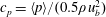
A second explanation for the different mean velocity profiles in experiment and simulation could be the wave damper we use in the experiment to damp surface waves. This is placed directly downstream of the flow straightener at the inflow into the water channel. This dampener slows down the flow at the surface and could lead to smaller surface velocities downstream, thus suppressing a pronounced wake profile. The first flow quantity on which the incoming flow profile will act is the downflow in front of the cylinder as it is induced by the velocity gradient in the incoming profile. We see that there are differences in the downflow in front of the cylinder (figure 8) which might also have an influence on the vortex system.
A comparison of the Reynolds normal stresses
 $\langle u^{\prime 2}\rangle$
and
$\langle u^{\prime 2}\rangle$
and
 $\langle w^{\prime 2}\rangle$
(figures 6
b and 6
c respectively) and the Reynolds shear stresses
$\langle w^{\prime 2}\rangle$
(figures 6
b and 6
c respectively) and the Reynolds shear stresses
 $\langle u^{\prime }w^{\prime }\rangle$
(figure 6
d) indicates accordance of the experimental and numerical inflow turbulence structures. The presented data also match the experimental data of Bruns, Dengel & Fernholz (Reference Bruns, Dengel and Fernholz1992) taken from Fernholz & Finley (Reference Fernholz and Finley1996) with similar Reynolds numbers based on the momentum thickness. Thus, we assume that the flow field of the approach flow is representative of a fully developed turbulent open-channel flow at the investigated Reynolds number. The overprediction of the vertical fluctuations
$\langle u^{\prime }w^{\prime }\rangle$
(figure 6
d) indicates accordance of the experimental and numerical inflow turbulence structures. The presented data also match the experimental data of Bruns, Dengel & Fernholz (Reference Bruns, Dengel and Fernholz1992) taken from Fernholz & Finley (Reference Fernholz and Finley1996) with similar Reynolds numbers based on the momentum thickness. Thus, we assume that the flow field of the approach flow is representative of a fully developed turbulent open-channel flow at the investigated Reynolds number. The overprediction of the vertical fluctuations
 $\langle w^{\prime 2}\rangle$
by the PIV in the near-wall region is a result of the coarse measurement resolution that was used when investigating the undisturbed flow.
$\langle w^{\prime 2}\rangle$
by the PIV in the near-wall region is a result of the coarse measurement resolution that was used when investigating the undisturbed flow.
In figure 6, we also include profiles measured under the slat that was placed at the water surface in front of the cylinder to provide optical access through the water surface. These measurements were made without the cylinder. The profiles have been averaged in time and space over a length of
 $1.25D$
in the middle of the slat. We observe that the influence of the slat is generally strong near the water surface but remains negligible below
$1.25D$
in the middle of the slat. We observe that the influence of the slat is generally strong near the water surface but remains negligible below
 $z^{+}<1000$
, which is approximately
$z^{+}<1000$
, which is approximately
 $z<D/3$
. Near the surface, the profiles measured with the slat seem to be smoother and less affected by artefacts than the ones measured without the slat. This can be explained by the smaller disturbance of the light sheet in the case with the slat.
$z<D/3$
. Near the surface, the profiles measured with the slat seem to be smoother and less affected by artefacts than the ones measured without the slat. This can be explained by the smaller disturbance of the light sheet in the case with the slat.

Figure 6. Time-averaged velocity profiles
 $\langle u\rangle /u_{\unicode[STIX]{x1D70F}}$
(a), streamwise Reynolds stress
$\langle u\rangle /u_{\unicode[STIX]{x1D70F}}$
(a), streamwise Reynolds stress
 $\langle u^{\prime 2}\rangle /u_{\unicode[STIX]{x1D70F}}^{2}$
(b), wall-normal Reynolds stress
$\langle u^{\prime 2}\rangle /u_{\unicode[STIX]{x1D70F}}^{2}$
(b), wall-normal Reynolds stress
 $\langle w^{\prime 2}\rangle /u_{\unicode[STIX]{x1D70F}}^{2}$
(c) and Reynolds shear stress
$\langle w^{\prime 2}\rangle /u_{\unicode[STIX]{x1D70F}}^{2}$
(c) and Reynolds shear stress
 $\langle u^{\prime }w^{\prime }\rangle /u_{\unicode[STIX]{x1D70F}}^{2}$
(d) in the precursor grid for PIV and LES. For reasons of visibility, only every third data point is plotted for
$\langle u^{\prime }w^{\prime }\rangle /u_{\unicode[STIX]{x1D70F}}^{2}$
(d) in the precursor grid for PIV and LES. For reasons of visibility, only every third data point is plotted for
 $z^{+}>150$
. The experimental data of Bruns et al. (Reference Bruns, Dengel and Fernholz1992) have been digitized from Fernholz & Finley (Reference Fernholz and Finley1996).
$z^{+}>150$
. The experimental data of Bruns et al. (Reference Bruns, Dengel and Fernholz1992) have been digitized from Fernholz & Finley (Reference Fernholz and Finley1996).
Throughout this paper, all values denoted as undisturbed or being from the incoming flow (for example
 $u_{b}$
,
$u_{b}$
,
 $\unicode[STIX]{x1D70F}_{0}$
or those presented in figure 6) are taken from the symmetry plane of the flume.
$\unicode[STIX]{x1D70F}_{0}$
or those presented in figure 6) are taken from the symmetry plane of the flume.

Figure 7. Streamlines of the time-averaged flow field in the symmetry plane in front of the cylinder for (a) PIV and (b) LES.
5.2 Horseshoe vortex system
Figure 7 presents the measured and simulated time-averaged streamlines in the symmetry plane in front of the cylinder. For both data sets, the seeding points defining the streamlines are uniformly distributed on a line between
 $(x,z)=(-1.2D,0)$
and
$(x,z)=(-1.2D,0)$
and
 $(x,z)=(-0.5D,0.2D)$
. From these seeding points, streamlines are integrated forwards as well as backwards in time. The approach flow profile leads to a vertical pressure gradient in front of the cylinder, which drives the downflow along the cylinder front. The main part of the downflow is turned upstream on reaching the bottom plate and flows upstream under the core of the main vortex V1. One part of this fluid is entrained into the main vortex; the other part forms a jet along the bottom wall directed against the main flow direction. The division between entrained fluid and fluid forming the jet is the stagnation point S1. The upstream-directed wall jet under S1 enters the upstream recirculation zone which ends at the critical point S2. We do not observe a second vortex V2 upstream of V1, in contrast to Apsilidis et al. (Reference Apsilidis, Diplas, Dancey and Bouratsis2015). The critical point S2 is not a separation as the fluid is not moving away from the wall at this point. The vertical velocity component in the vicinity of this point is negative. Instead, it renders itself as a sink in the 2D symmetry plane, which would be a stagnation point in 3D. This finding is different from the commonly used term ‘separation’ for this critical point and from the topology sketches of Baker (Reference Baker1979) for laminar flows. A discussion on the flow topology can be found in Simpson (Reference Simpson2001). We cannot explain the different topology compared with that documented by Apsilidis et al. (Reference Apsilidis, Diplas, Dancey and Bouratsis2015), but suggest that the state of the turbulent boundary layer approaching the obstacle might be a key factor determining whether the point of first flow reversal in front of an obstacle will be a point of separation or a stagnation point.
$(x,z)=(-0.5D,0.2D)$
. From these seeding points, streamlines are integrated forwards as well as backwards in time. The approach flow profile leads to a vertical pressure gradient in front of the cylinder, which drives the downflow along the cylinder front. The main part of the downflow is turned upstream on reaching the bottom plate and flows upstream under the core of the main vortex V1. One part of this fluid is entrained into the main vortex; the other part forms a jet along the bottom wall directed against the main flow direction. The division between entrained fluid and fluid forming the jet is the stagnation point S1. The upstream-directed wall jet under S1 enters the upstream recirculation zone which ends at the critical point S2. We do not observe a second vortex V2 upstream of V1, in contrast to Apsilidis et al. (Reference Apsilidis, Diplas, Dancey and Bouratsis2015). The critical point S2 is not a separation as the fluid is not moving away from the wall at this point. The vertical velocity component in the vicinity of this point is negative. Instead, it renders itself as a sink in the 2D symmetry plane, which would be a stagnation point in 3D. This finding is different from the commonly used term ‘separation’ for this critical point and from the topology sketches of Baker (Reference Baker1979) for laminar flows. A discussion on the flow topology can be found in Simpson (Reference Simpson2001). We cannot explain the different topology compared with that documented by Apsilidis et al. (Reference Apsilidis, Diplas, Dancey and Bouratsis2015), but suggest that the state of the turbulent boundary layer approaching the obstacle might be a key factor determining whether the point of first flow reversal in front of an obstacle will be a point of separation or a stagnation point.
The downwash at the cylinder front establishes a thin boundary layer at the flow-facing wall of the cylinder, which results in a pressure gradient between stagnation point S3 and the cylinder–wall junction. Thus, a small part of the fluid pushed downwards in front of the cylinder is deflected towards the cylinder on reaching the bottom plate, forming the corner vortex V3. The stagnation point S3 separates the fluid pointing in the upstream direction from that flowing towards the cylinder. The corner vortex V3 is trapped between stagnation point S3 and the cylinder–wall junction. The PIV flow field (figure 7 a) illustrates the similarity between V1, S1 and V3, S4 respectively. One could speculate that at higher Reynolds numbers, or with a better spatial resolution, a cascade of more and more smaller vortices appear in the corner between the cylinder and the wall, which would be cut due to viscous effects. In fact, such an additional corner vortex is visible in the streamline plots of Ryu et al. (Reference Ryu, Emory, Iaccarino, Campos and Duraisamy2016), who simulated the wing–plate junction flow case of Devenport & Simpson (Reference Devenport and Simpson1990), which has a higher Reynolds number than the one of our case. Our single-pixel results for the time-averaged wall shear stress (§ 5.3, figure 11) show another small zone of negative wall shear stress just in front of the cylinder, which suggests a small clockwise-rotating vortex in front of the cylinder. This would be in line with the streamline plot of Ryu et al. (Reference Ryu, Emory, Iaccarino, Campos and Duraisamy2016).
Between the stagnation points S3 and S2, the flow is pointing upstream along the wall, forming a wall jet, as discussed above. The upstream-directed flow is subject to a distinct pattern of acceleration along the streamlines. The rate of change of the distance between two adjacent streamlines is a measure for the velocity acceleration. As streamlines move together in figure 7, the flow accelerates, and vice versa. In particular, upstream of the stagnation point S3 in the range
 $-0.73D<x<-0.53D$
, we can observe strong acceleration of the near-wall flow. After passing under the vortex V1, the spacing of the streamlines widens slightly, indicating deceleration. Finally, the fluid reaccelerates towards S2 or to being transported out of the plane in the spanwise direction. The consequences of this acceleration pattern on the budget of turbulent kinetic energy will be discussed in § 6.
$-0.73D<x<-0.53D$
, we can observe strong acceleration of the near-wall flow. After passing under the vortex V1, the spacing of the streamlines widens slightly, indicating deceleration. Finally, the fluid reaccelerates towards S2 or to being transported out of the plane in the spanwise direction. The consequences of this acceleration pattern on the budget of turbulent kinetic energy will be discussed in § 6.
The exact locations of the critical points mentioned above are listed in table 2. Comparison of the locations evaluated by PIV and LES shows satisfying accordance. However, the comparison of the streamlines in figure 7 points out a slight difference. In the LES, more fluid is entrained by the main vortex V1, resulting in the vortex being optically larger (figure 7
b). The streamline approaching S1 from upstream originates from
 $z/D=0.05$
in both cases. The streamline approaching S1 from downstream emanates from
$z/D=0.05$
in both cases. The streamline approaching S1 from downstream emanates from
 $z/D\approx 0.11$
in the experiment and from
$z/D\approx 0.11$
in the experiment and from
 $z/D\approx 0.16$
in the LES. This is the streamline separating the fluid under the main vortex V1 into fluid going upstream along the wall and fluid being entrained into the vortex.
$z/D\approx 0.16$
in the LES. This is the streamline separating the fluid under the main vortex V1 into fluid going upstream along the wall and fluid being entrained into the vortex.
Table 2. The positions of the critical points. If no
 $z_{Si}$
is given, the corresponding stagnation point is located at the bottom plate.
$z_{Si}$
is given, the corresponding stagnation point is located at the bottom plate.
Figure 8 compares the streamwise profiles of the time-averaged vertical velocity component
 $\langle w\rangle$
from LES and PIV on a horizontal line at
$\langle w\rangle$
from LES and PIV on a horizontal line at
 $z_{V1}=0.06D$
, which is through the centre of the main vortex V1. Negative values imply downflow, and vice versa. The experimental data in single-pixel resolution (dots) were smoothed by applying a moving spatial filter over 16 px (solid line).
$z_{V1}=0.06D$
, which is through the centre of the main vortex V1. Negative values imply downflow, and vice versa. The experimental data in single-pixel resolution (dots) were smoothed by applying a moving spatial filter over 16 px (solid line).
Vortex V1 can be identified in figure 8, as the upward-directed flow upstream and the downflow downstream from
 $x_{V1}$
indicate a clockwise rotation. The zero crossings between
$x_{V1}$
indicate a clockwise rotation. The zero crossings between
 $x/D=-0.8$
and
$x/D=-0.8$
and
 $x/D=-0.7$
indicate the location of the vortex centre. The downflow between the vortex centre and the cylinder shows two local minima separated by a local maximum which is at approximately
$x/D=-0.7$
indicate the location of the vortex centre. The downflow between the vortex centre and the cylinder shows two local minima separated by a local maximum which is at approximately
 $x\approx -0.6D$
.
$x\approx -0.6D$
.
There is a qualitative match between the measured and simulated profiles. However, the vortex centre is more upstream in the experiment, which leads to a larger extent of the downflow region. In addition, the magnitude of the downflow is larger in the experiment. We observe that the single-pixel evaluation gives results qualitatively closer to the LES than the standard PIV. The standard PIV does not show the second local minimum at approximately
 $x/D=-0.65$
and gives visibly larger vertical velocities in the zone upstream of the vortex core than single-pixel PIV. There might be some small-scale events contributing to the time-averaged flow field which cannot be resolved by the relatively large interrogation windows of the standard PIV.
$x/D=-0.65$
and gives visibly larger vertical velocities in the zone upstream of the vortex core than single-pixel PIV. There might be some small-scale events contributing to the time-averaged flow field which cannot be resolved by the relatively large interrogation windows of the standard PIV.

Figure 8. Profiles of the wall-normal velocity component
 $\langle w\rangle$
in the symmetry plane in front of the cylinder at a wall distance of
$\langle w\rangle$
in the symmetry plane in front of the cylinder at a wall distance of
 $z_{V1}=0.06D$
.
$z_{V1}=0.06D$
.

Figure 9. Streamlines of the time-averaged flow field (a) and the pressure distribution
 $c_{p}=\langle p\rangle /(0.5\unicode[STIX]{x1D70C}u_{b}^{2})$
(b) along the bottom plate around the cylinder taken from the LES.
$c_{p}=\langle p\rangle /(0.5\unicode[STIX]{x1D70C}u_{b}^{2})$
(b) along the bottom plate around the cylinder taken from the LES.
Figure 9(a) shows a top view of the simulated streamlines along the bottom plate, i.e. taking the stream- and spanwise velocities at
 $z=0.001D$
. The streamlines are integrated back in time from points distributed equidistantly on a spanwise line at
$z=0.001D$
. The streamlines are integrated back in time from points distributed equidistantly on a spanwise line at
 $x=0.8D$
. This results in a relatively loose package of streamlines in the cylinder front. The regions dominated by the different vortices are visible here. The thin blank ring around the cylinder marks the corner vortex V3 in which fluid moves from the stagnation line towards the cylinder. The stagnation line collects streamlines which are integrated back in time from the points defined by the probe and go through the stagnation point S3 in the symmetry plane. Upstream of S3, the fluid moves in the upstream direction in a nearly straight manner, i.e. the streamlines close to the symmetry plane between S3 and
$x=0.8D$
. This results in a relatively loose package of streamlines in the cylinder front. The regions dominated by the different vortices are visible here. The thin blank ring around the cylinder marks the corner vortex V3 in which fluid moves from the stagnation line towards the cylinder. The stagnation line collects streamlines which are integrated back in time from the points defined by the probe and go through the stagnation point S3 in the symmetry plane. Upstream of S3, the fluid moves in the upstream direction in a nearly straight manner, i.e. the streamlines close to the symmetry plane between S3 and
 $x/D\approx -0.75$
are nearly parallel. This indicates that almost all of the fluid close to the symmetry plane remains there and the transport in the spanwise direction is small underneath V1. The transport in the spanwise direction starts in the deceleration region of the wall jet at
$x/D\approx -0.75$
are nearly parallel. This indicates that almost all of the fluid close to the symmetry plane remains there and the transport in the spanwise direction is small underneath V1. The transport in the spanwise direction starts in the deceleration region of the wall jet at
 $x\approx -0.8D$
, where the streamlines bear strong curvature, implying that major parts of the fluid leave the symmetry plane.
$x\approx -0.8D$
, where the streamlines bear strong curvature, implying that major parts of the fluid leave the symmetry plane.
The streamlines along the bottom plate are linked to the pressure distribution on the bottom plate, shown as pressure coefficient
 $c_{p}=\langle p\rangle /(0.5\unicode[STIX]{x1D70C}u_{b}^{2})$
in figure 9(b). Large pressure is indicated by dark colour and small pressure is indicated by light colour. The largest pressure is observed in front of the cylinder where the downflow hits the bottom plate between the main vortex and the cylinder. The near-wall streamlines in this area are pointing upstream in the direction of the steepest pressure gradient. At
$c_{p}=\langle p\rangle /(0.5\unicode[STIX]{x1D70C}u_{b}^{2})$
in figure 9(b). Large pressure is indicated by dark colour and small pressure is indicated by light colour. The largest pressure is observed in front of the cylinder where the downflow hits the bottom plate between the main vortex and the cylinder. The near-wall streamlines in this area are pointing upstream in the direction of the steepest pressure gradient. At
 $x\approx -0.8D$
, the pressure gradient is of similar magnitude in both the upstream and spanwise directions, causing the fluid to be transported outwards from the symmetry plane. At the same location, the streamlines in figure 9(a) bear the largest curvature and deviate from the symmetry plane. The stagnation line from point S3 would be visible in radial pressure profiles as local maxima.
$x\approx -0.8D$
, the pressure gradient is of similar magnitude in both the upstream and spanwise directions, causing the fluid to be transported outwards from the symmetry plane. At the same location, the streamlines in figure 9(a) bear the largest curvature and deviate from the symmetry plane. The stagnation line from point S3 would be visible in radial pressure profiles as local maxima.

Figure 10. Top views of the instantaneous three-dimensional vortex structure visualized by
 $Qu_{b}^{2}/D^{2}=1000$
taken from the LES. In each panel, two realizations at arbitrary times have been plotted on top of each other.
$Qu_{b}^{2}/D^{2}=1000$
taken from the LES. In each panel, two realizations at arbitrary times have been plotted on top of each other.
Further insight into the three-dimensional behaviour of the vortex system can be gained from the instantaneous distributions of the second invariant of the velocity gradient tensor (figure 10). This so-called
 $Q$
-criterion is widely used to visualize vortex structures. The isosurfaces
$Q$
-criterion is widely used to visualize vortex structures. The isosurfaces
 $Qu_{b}^{2}/D^{2}=1000$
are rendered in a volume between
$Qu_{b}^{2}/D^{2}=1000$
are rendered in a volume between
 $z=0$
and
$z=0$
and
 $z=0.2D$
. The value was chosen to enable the identification of vortical structures. In each panel, we overlay two arbitrary time instants to demonstrate the spatial variability of the horseshoe vortex. The isosurface of
$z=0.2D$
. The value was chosen to enable the identification of vortical structures. In each panel, we overlay two arbitrary time instants to demonstrate the spatial variability of the horseshoe vortex. The isosurface of
 $Q$
at one instant is rendered in black and the other one in grey. In figure 10(a), the wakes behind the cylinder are approximately symmetric. In figure 10(b), the two instants are chosen to be during vortex shedding, i.e. the wakes are asymmetric and the vortices are shedding from opposite sides of the cylinder at the two instants.
$Q$
at one instant is rendered in black and the other one in grey. In figure 10(a), the wakes behind the cylinder are approximately symmetric. In figure 10(b), the two instants are chosen to be during vortex shedding, i.e. the wakes are asymmetric and the vortices are shedding from opposite sides of the cylinder at the two instants.
At all four instants, the main vortex V1 is visible in front (on the left) of the cylinder. It bends around the cylinder like a horseshoe. The four instants demonstrate that the horseshoe vortex can undergo parallel displacements in the streamwise direction, as visible in figure 10(a), and a tilting around a vertical axis, as visible in figure 10(b). The displacement between the two instants in figure 10(a) is relatively large. The streamwise positions of the cores in the symmetry plane are
 $x/D\approx -0.83$
and
$x/D\approx -0.83$
and
 $x/D\approx -0.7$
respectively. In figure 10(b), both vortices are at the same streamwise position in the symmetry plane at
$x/D\approx -0.7$
respectively. In figure 10(b), both vortices are at the same streamwise position in the symmetry plane at
 $x/D\approx -0.73$
, which is the position of the time-averaged vortex V1. Small secondary vortices are visible at all instants, wrapping around the horseshoe vortex. It seems that they are lifted up upstream of the horseshoe vortex, which is in the region in which the upstream jet under the vortex decelerates. A deceleration of the streamwise velocity component and simultaneous stretching in the vertical direction would give rise to vertical vorticity, which is manifested here in the secondary vortices which mainly occur upstream of the horseshoe vortex. Downstream of the horseshoe vortex, between the vortex and the cylinder, the instantaneous vortical structures render a calm region at all times in the sense that no intense vortices are visible.
$x/D\approx -0.73$
, which is the position of the time-averaged vortex V1. Small secondary vortices are visible at all instants, wrapping around the horseshoe vortex. It seems that they are lifted up upstream of the horseshoe vortex, which is in the region in which the upstream jet under the vortex decelerates. A deceleration of the streamwise velocity component and simultaneous stretching in the vertical direction would give rise to vertical vorticity, which is manifested here in the secondary vortices which mainly occur upstream of the horseshoe vortex. Downstream of the horseshoe vortex, between the vortex and the cylinder, the instantaneous vortical structures render a calm region at all times in the sense that no intense vortices are visible.
The instants rendered in figure 10 do not represent a time sequence. However, one observation can be made on the coherence of the horseshoe vortex. If the vortex is at the position closest to the cylinder, the vortex is a coherent tube over a long distance along its core. If the vortex is at the position farthest away from the cylinder, the vortex cannot really be identified as a coherent single vortex. It is more or less a disordered arrangement of small-scaled vortices arranged along a curve in space that resembles a horseshoe vortex. This stage might be what results from a destabilization of the vortex by secondary vortices wrapped around the main vortex.
The vortex structures rendered in figure 10 are quite different from the instantaneous vortical structures documented by Escauriaza & Sotiropoulos (Reference Escauriaza and Sotiropoulos2011) for detached eddy simulations, but consistent with the structures described by Apsilidis et al. (Reference Apsilidis, Khosronejad, Sotiropoulos, Dancey and Diplas2012) for LES.
5.3 Wall shear stress distribution
The flow described above exerts a specific pattern of wall shear stress on the bottom plate. Figure 11 shows the friction coefficient
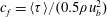 $c_{f}=\langle \unicode[STIX]{x1D70F}\rangle /(0.5\unicode[STIX]{x1D70C}u_{b}^{2})$
in the symmetry plane upstream of the cylinder. The friction factor is negative in the large back-flow zone between the two stagnation points S2 and S3 (figure 7) and positive in the forward flow between the stagnation point S3 (
$c_{f}=\langle \unicode[STIX]{x1D70F}\rangle /(0.5\unicode[STIX]{x1D70C}u_{b}^{2})$
in the symmetry plane upstream of the cylinder. The friction factor is negative in the large back-flow zone between the two stagnation points S2 and S3 (figure 7) and positive in the forward flow between the stagnation point S3 (
 $x/D\approx -0.53$
) and the cylinder wall.
$x/D\approx -0.53$
) and the cylinder wall.

Figure 11. The distribution of the friction coefficient
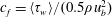 $c_{f}=\langle \unicode[STIX]{x1D70F}_{w}\rangle /(0.5\unicode[STIX]{x1D70C}u_{b}^{2})$
over
$c_{f}=\langle \unicode[STIX]{x1D70F}_{w}\rangle /(0.5\unicode[STIX]{x1D70C}u_{b}^{2})$
over
 $x/D$
in the symmetry plane in front of the cylinder.
$x/D$
in the symmetry plane in front of the cylinder.
The footprints of the two vortices discussed above, V1 and V3, are visible in the distributions of
 $c_{f}$
. The anticlockwise-rotating vortex V3 causes the strong positive wall shear stress peak at
$c_{f}$
. The anticlockwise-rotating vortex V3 causes the strong positive wall shear stress peak at
 $-0.53D<x<-0.5D$
. The stagnation point S3 is located where the wall shear stress is zero at
$-0.53D<x<-0.5D$
. The stagnation point S3 is located where the wall shear stress is zero at
 $x\approx -0.53D$
. Upstream of S3, the acceleration zone of the described wall jet leads to the broad region of negative wall shear stress at
$x\approx -0.53D$
. Upstream of S3, the acceleration zone of the described wall jet leads to the broad region of negative wall shear stress at
 $-0.8D<x<-0.53D$
. It should be noted that the maximum magnitudes of the wall shear stress are not found under the vortex core of the horseshoe vortex V1 but in the zone in which the flow is accelerated between stagnation point S3 and the location under the vortex core V1. Under the stagnation point S1, there is a local maximum of the wall shear stress, which means that the magnitude of the wall shear stress has a local minimum as the flow is pointing upstream. We do not observe a local recirculation embedded in this upstream flow as other authors have reported (e.g. Escauriaza & Sotiropoulos Reference Escauriaza and Sotiropoulos2011). The upstream jet forming under the main horseshoe vortex V1 reaches up to the stagnation point S2 at
$-0.8D<x<-0.53D$
. It should be noted that the maximum magnitudes of the wall shear stress are not found under the vortex core of the horseshoe vortex V1 but in the zone in which the flow is accelerated between stagnation point S3 and the location under the vortex core V1. Under the stagnation point S1, there is a local maximum of the wall shear stress, which means that the magnitude of the wall shear stress has a local minimum as the flow is pointing upstream. We do not observe a local recirculation embedded in this upstream flow as other authors have reported (e.g. Escauriaza & Sotiropoulos Reference Escauriaza and Sotiropoulos2011). The upstream jet forming under the main horseshoe vortex V1 reaches up to the stagnation point S2 at
 $x\approx -1.1D$
. This observation can be made for both experiment and simulation, and is consistent with findings by Devenport & Simpson (Reference Devenport and Simpson1990).
$x\approx -1.1D$
. This observation can be made for both experiment and simulation, and is consistent with findings by Devenport & Simpson (Reference Devenport and Simpson1990).
As illustrated in figure 9, major parts of the fluid are leaving the symmetry plane and accelerating in the spanwise direction in the zone
 $-1.1D<x<-0.8D$
, which is approximately between the stagnation point S2 and the main vortex core. This could explain why the wall shear stress between V1 and S2 is much smaller than that underneath vortex V1. The local maximum of the amplitude at
$-1.1D<x<-0.8D$
, which is approximately between the stagnation point S2 and the main vortex core. This could explain why the wall shear stress between V1 and S2 is much smaller than that underneath vortex V1. The local maximum of the amplitude at
 $x\approx -0.9D$
could be explained by the fluid pointing towards the wall upstream of S1.
$x\approx -0.9D$
could be explained by the fluid pointing towards the wall upstream of S1.
The numerical results are documented for three simulations with different grid resolutions. The simulation denoted as level 1 holds one locally embedded grid only, and the wall distance of the wall-parallel velocity is
 $0.002D$
. Since simulation level 2 has two locally embedded grids, the grid spacing around the cylinder is reduced by a factor of two compared with simulation level 1, which leads to a wall distance of the first velocity of
$0.002D$
. Since simulation level 2 has two locally embedded grids, the grid spacing around the cylinder is reduced by a factor of two compared with simulation level 1, which leads to a wall distance of the first velocity of
 $0.001D$
. In simulation level 3, the grid spacing is further reduced by a factor of two and the wall distance is
$0.001D$
. In simulation level 3, the grid spacing is further reduced by a factor of two and the wall distance is
 $5\times 10^{-4}D$
. Here, the grid is eight times finer than in the precursor and the base grid. The differences between the wall shear stress taken from the simulation with the coarse grid (level 1) and from the one with the medium grid (level 2) are significant. The coarse grid underestimates the amplitude of
$5\times 10^{-4}D$
. Here, the grid is eight times finer than in the precursor and the base grid. The differences between the wall shear stress taken from the simulation with the coarse grid (level 1) and from the one with the medium grid (level 2) are significant. The coarse grid underestimates the amplitude of
 $c_{f}$
under the wall jet. Furthermore, it is not able to capture the double peak in the region of large wall shear stress. Obviously, it is also too coarse to resolve vortex V3, as
$c_{f}$
under the wall jet. Furthermore, it is not able to capture the double peak in the region of large wall shear stress. Obviously, it is also too coarse to resolve vortex V3, as
 $c_{f}$
shows no positive peak right in front of the cylinder. In contrast, the differences between the simulations with the medium grid (level 2) and the fine grid (level 3) are rather small. Both exhibit approximately the same amplitude and capture the double peak distribution under the wall jet between
$c_{f}$
shows no positive peak right in front of the cylinder. In contrast, the differences between the simulations with the medium grid (level 2) and the fine grid (level 3) are rather small. Both exhibit approximately the same amplitude and capture the double peak distribution under the wall jet between
 $-0.7D<x<-0.55D$
. We thus consider the flow to be satisfyingly converged over grid refinement. The grid dependence of the presented LES is discussed in more detail by Schanderl & Manhart (Reference Schanderl and Manhart2016). All numerical data relating to the region around the cylinder presented in this paper are taken from the simulation with the fine grid (level 3). It should be noted that the data characterizing the inflow (§ 5.1) stem from level zero, since no local grid refinement is applied in the precursor grid.
$-0.7D<x<-0.55D$
. We thus consider the flow to be satisfyingly converged over grid refinement. The grid dependence of the presented LES is discussed in more detail by Schanderl & Manhart (Reference Schanderl and Manhart2016). All numerical data relating to the region around the cylinder presented in this paper are taken from the simulation with the fine grid (level 3). It should be noted that the data characterizing the inflow (§ 5.1) stem from level zero, since no local grid refinement is applied in the precursor grid.
The experimental data are documented for both a standard interrogation window and a single-pixel evaluation. The standard method results have a wall distance of at least
 $0.0019D$
, which is half of the interrogation window size. The results obtained are in line with the LES results at a comparable grid spacing, level 1. The dual-peak nature of the strong wall shear stress is not reproduced by these results. The wall distance of the first valid single-pixel vectors is limited by half of the diameter of a particle image (Kähler, Scharnowski & Cierpka Reference Kähler, Scharnowski and Cierpka2012), which is 3.4 px. With a pixel size of
$0.0019D$
, which is half of the interrogation window size. The results obtained are in line with the LES results at a comparable grid spacing, level 1. The dual-peak nature of the strong wall shear stress is not reproduced by these results. The wall distance of the first valid single-pixel vectors is limited by half of the diameter of a particle image (Kähler, Scharnowski & Cierpka Reference Kähler, Scharnowski and Cierpka2012), which is 3.4 px. With a pixel size of
 $48~\unicode[STIX]{x03BC}\text{m}$
, this gives a wall distance of approximately
$48~\unicode[STIX]{x03BC}\text{m}$
, this gives a wall distance of approximately
 $8\times 10^{-4}D$
, which is between the wall distances of the finest and second finest LES. Since the single-pixel method is more sensitive to statistics and measurement issues, the corresponding wall shear stress distribution shows significant scatter. However, neglecting these oscillations, the single-pixel data support both the amplitude and the shape of the LES results.
$8\times 10^{-4}D$
, which is between the wall distances of the finest and second finest LES. Since the single-pixel method is more sensitive to statistics and measurement issues, the corresponding wall shear stress distribution shows significant scatter. However, neglecting these oscillations, the single-pixel data support both the amplitude and the shape of the LES results.
While the overall behaviour of the wall shear stress agrees well between LES (level 3) and standard
 $16\times 16$
px PIV, a detailed look reveals subtle differences. The LES predicts two local wall shear stress minima in the main recirculation zone and a plateau between them. The standard PIV, however, shows only the minimum at
$16\times 16$
px PIV, a detailed look reveals subtle differences. The LES predicts two local wall shear stress minima in the main recirculation zone and a plateau between them. The standard PIV, however, shows only the minimum at
 $x/D\approx -0.7$
and no plateau. The measured distribution of the wall shear stress between
$x/D\approx -0.7$
and no plateau. The measured distribution of the wall shear stress between
 $x/D=-0.7$
and
$x/D=-0.7$
and
 $x/D=-0.53$
resembles the one documented by Roulund et al. (Reference Roulund, Sumer, Fredsoe and Michelsen2005) for a similar configuration at
$x/D=-0.53$
resembles the one documented by Roulund et al. (Reference Roulund, Sumer, Fredsoe and Michelsen2005) for a similar configuration at
 $Re_{D}=170\,000$
. However, application of the single-pixel method to the experimental data reveals a similar plateau to that in the LES (level 3).
$Re_{D}=170\,000$
. However, application of the single-pixel method to the experimental data reveals a similar plateau to that in the LES (level 3).
Under V3 (
 $x/D>-0.53$
), the amplitude of
$x/D>-0.53$
), the amplitude of
 $c_{f}$
is largest in the single-pixel data, while the wall shear stress from the standard PIV is smallest. The amplitude increases with the data resolution here. This suggests that both LES and standard PIV are too coarse to resolve vortex V3 sufficiently. Furthermore, the single-pixel PIV shows negative values directly at the cylinder. This aspect is in favour of the possibility of an additional vortex rotating in the clockwise direction, as discussed in § 5.2.
$c_{f}$
is largest in the single-pixel data, while the wall shear stress from the standard PIV is smallest. The amplitude increases with the data resolution here. This suggests that both LES and standard PIV are too coarse to resolve vortex V3 sufficiently. Furthermore, the single-pixel PIV shows negative values directly at the cylinder. This aspect is in favour of the possibility of an additional vortex rotating in the clockwise direction, as discussed in § 5.2.
6 Turbulence structure
The horseshoe vortex system is subject to strong fluctuations, as documented by several authors, e.g. Devenport & Simpson (Reference Devenport and Simpson1990), Escauriaza & Sotiropoulos (Reference Escauriaza and Sotiropoulos2011) and Apsilidis et al. (Reference Apsilidis, Diplas, Dancey and Bouratsis2015). Furthermore, it has been demonstrated that the near-wall momentum balance under the horseshoe vortex and especially in the large-magnitude shear stress region under the downflow is dominated by the convective terms. Reynolds stresses play a minor role here (Schanderl & Manhart Reference Schanderl and Manhart2015). To gain further insight into the dynamics of the vortex system, we investigate the turbulence structure in this section. We restrict ourselves to an analysis in a statistical sense, including the turbulent kinetic energy, Reynolds stresses, and their production, dissipation and diffusion.
6.1 Turbulent kinetic energy

Figure 12. The turbulent kinetic energy in the symmetry plane in front of the cylinder: the in-plane turbulent kinetic energy
 $k_{ip}/u_{b}^{2}$
measured by PIV (a) and simulated by LES (b); the full turbulent kinetic energy
$k_{ip}/u_{b}^{2}$
measured by PIV (a) and simulated by LES (b); the full turbulent kinetic energy
 $k/u_{b}^{2}$
simulated by LES (c).
$k/u_{b}^{2}$
simulated by LES (c).

Figure 13. Reynolds stresses in the symmetry plane in front of the cylinder obtained from LES:
 $\langle u^{\prime 2}\rangle /u_{b}^{2}$
(a),
$\langle u^{\prime 2}\rangle /u_{b}^{2}$
(a),
 $\langle w^{\prime 2}\rangle /u_{b}^{2}$
(b) and
$\langle w^{\prime 2}\rangle /u_{b}^{2}$
(b) and
 $\langle u^{\prime }w^{\prime }\rangle /u_{b}^{2}$
(c).
$\langle u^{\prime }w^{\prime }\rangle /u_{b}^{2}$
(c).
All previously published works report an enhanced level of turbulent kinetic energy (4.1) near the core of the main horseshoe vortex V1. At moderate Reynolds numbers, such as the one considered here, the main observation is that the distribution of the turbulent kinetic energy follows a characteristic c-shape. There is a main peak around the vortex core V1 and a leg-like structure between the main peak and the bottom wall.
This structure can also be seen in our results (figure 12). The in-plane turbulent kinetic energy
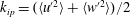 $k_{ip}=(\langle u^{\prime 2}\rangle +\langle w^{\prime 2}\rangle )/2$
(figure 12
b) is a fairly good representation of the full turbulent kinetic energy (figure 12
c). However, the peak value in the horseshoe vortex core of the full turbulent kinetic energy is approximately 20 % larger than the one of the in-plane turbulent kinetic energy. In contrast to the LES results (figure 12
b,c), the position of the corner vortex V3 is visible in the PIV results (figure 12
a). Overall, the measured peak values of the turbulent kinetic energy are approximately 20 %–30 % larger than the simulated ones and similar to the ones reported for
$k_{ip}=(\langle u^{\prime 2}\rangle +\langle w^{\prime 2}\rangle )/2$
(figure 12
b) is a fairly good representation of the full turbulent kinetic energy (figure 12
c). However, the peak value in the horseshoe vortex core of the full turbulent kinetic energy is approximately 20 % larger than the one of the in-plane turbulent kinetic energy. In contrast to the LES results (figure 12
b,c), the position of the corner vortex V3 is visible in the PIV results (figure 12
a). Overall, the measured peak values of the turbulent kinetic energy are approximately 20 %–30 % larger than the simulated ones and similar to the ones reported for
 $Re_{D}=47\,000$
by Apsilidis et al. (Reference Apsilidis, Diplas, Dancey and Bouratsis2015).
$Re_{D}=47\,000$
by Apsilidis et al. (Reference Apsilidis, Diplas, Dancey and Bouratsis2015).
For a detailed view, we investigate the individual Reynolds stresses. We restrict ourselves to presenting the LES results only, as there are minor differences between the measured and simulated distributions. The Reynolds normal stresses in the streamwise direction
 $\langle u^{\prime 2}\rangle$
contribute mainly to the leg of the turbulent kinetic energy distribution (figure 13
a). This leg is located in the near-wall jet underneath the main vortex core. Following the streamlines from the downflow between the vortex V1 and the cylinder (compare figure 7), the streamwise turbulence intensity grows considerably when the local acceleration, as indicated by converging streamlines, diminishes (at
$\langle u^{\prime 2}\rangle$
contribute mainly to the leg of the turbulent kinetic energy distribution (figure 13
a). This leg is located in the near-wall jet underneath the main vortex core. Following the streamlines from the downflow between the vortex V1 and the cylinder (compare figure 7), the streamwise turbulence intensity grows considerably when the local acceleration, as indicated by converging streamlines, diminishes (at
 $x\approx -0.75D$
). The measured level of
$x\approx -0.75D$
). The measured level of
 $\langle u^{\prime 2}\rangle$
is in general slightly larger than the numerical one.
$\langle u^{\prime 2}\rangle$
is in general slightly larger than the numerical one.
The vertical Reynolds normal stress
 $\langle w^{\prime 2}\rangle$
(figure 13
b) peaks approximately around the centre of V1, which is consistent with horizontal variations of the main vortex core. Both LES and PIV have similar amplitudes. In addition to the peak around the horseshoe vortex, we can observe enhanced vertical Reynolds stresses in a band along the front of the cylinder in both LES and PIV.
$\langle w^{\prime 2}\rangle$
(figure 13
b) peaks approximately around the centre of V1, which is consistent with horizontal variations of the main vortex core. Both LES and PIV have similar amplitudes. In addition to the peak around the horseshoe vortex, we can observe enhanced vertical Reynolds stresses in a band along the front of the cylinder in both LES and PIV.
Finally, the Reynolds shear stress
 $\langle u^{\prime }w^{\prime }\rangle$
is presented in figure 13(c). There is a large patch with negative shear stress in the left half of vortex V1 slightly downstream of the stagnation point S1, and a patch of positive shear stress downstream of the main vortex.
$\langle u^{\prime }w^{\prime }\rangle$
is presented in figure 13(c). There is a large patch with negative shear stress in the left half of vortex V1 slightly downstream of the stagnation point S1, and a patch of positive shear stress downstream of the main vortex.

Figure 14. Isosurfaces of the turbulent kinetic energy in the cylinder front taken from the LES;
 $k/u_{b}^{2}=0.035$
is marked in red and
$k/u_{b}^{2}=0.035$
is marked in red and
 $k/u_{b}^{2}=0.07$
is marked in blue. The former is only shown up to the symmetry plane.
$k/u_{b}^{2}=0.07$
is marked in blue. The former is only shown up to the symmetry plane.
Figure 14 illustrates three-dimensional isosurfaces of
 $k/u_{b}^{2}=0.035$
(red) and
$k/u_{b}^{2}=0.035$
(red) and
 $k/u_{b}^{2}=0.07$
(blue) in the cylinder front. The isosurface of
$k/u_{b}^{2}=0.07$
(blue) in the cylinder front. The isosurface of
 $k/u_{b}^{2}=0.035$
encloses the region covered by the main vortex V1, while values of
$k/u_{b}^{2}=0.035$
encloses the region covered by the main vortex V1, while values of
 $k/u_{b}^{2}>0.07$
are limited to its core. When V1 is bent around the cylinder and the fluid accelerates, the cross-sectional area enclosed by the isosurfaces shrinks. Furthermore, it is noticeable that in the region between V1 and the cylinder, the turbulent kinetic energy is relatively small. This is the zone where the downflow in front of the cylinder takes place. In the following sections, we further discuss this issue by taking a deeper look at the balance equation of the turbulent kinetic energy.
$k/u_{b}^{2}>0.07$
are limited to its core. When V1 is bent around the cylinder and the fluid accelerates, the cross-sectional area enclosed by the isosurfaces shrinks. Furthermore, it is noticeable that in the region between V1 and the cylinder, the turbulent kinetic energy is relatively small. This is the zone where the downflow in front of the cylinder takes place. In the following sections, we further discuss this issue by taking a deeper look at the balance equation of the turbulent kinetic energy.
6.2 Turbulent kinetic energy balance
In the remainder of this paper, we will investigate the complete budget of the turbulent kinetic energy
 $k$
(4.1) in front of the wall-mounted cylinder. According to, e.g., Pope (Reference Pope2011), the budget contains convection by the time-averaged flow
$k$
(4.1) in front of the wall-mounted cylinder. According to, e.g., Pope (Reference Pope2011), the budget contains convection by the time-averaged flow
 $C$
, turbulent convection
$C$
, turbulent convection
 $T_{conv}$
, pressure transport
$T_{conv}$
, pressure transport
 $T_{pres}$
, viscous diffusion
$T_{pres}$
, viscous diffusion
 $T_{visc}$
, production
$T_{visc}$
, production
 $P$
and dissipation
$P$
and dissipation
 $\unicode[STIX]{x1D716}$
,
$\unicode[STIX]{x1D716}$
,
 $$\begin{eqnarray}0=C+T_{conv}+T_{pres}+T_{visc}+P-\unicode[STIX]{x1D716}.\end{eqnarray}$$
In a statistically steady flow, the convective term
 $C$
reads as
$C$
reads as
 $$\begin{eqnarray}C=-\langle u_{i}\rangle \frac{\unicode[STIX]{x2202}k}{\unicode[STIX]{x2202}x_{i}}.\end{eqnarray}$$
Besides the mean convection
 $C$
, three mechanisms are responsible for redistributing
$C$
, three mechanisms are responsible for redistributing
 $k$
in space: turbulent convection
$k$
in space: turbulent convection
 $T_{conv}$
, pressure transport
$T_{conv}$
, pressure transport
 $T_{pres}$
and viscous diffusion
$T_{pres}$
and viscous diffusion
 $T_{visc}$
,
$T_{visc}$
,
 $$\begin{eqnarray}\displaystyle & \displaystyle T_{conv}=-\frac{1}{2}\frac{\unicode[STIX]{x2202}}{\unicode[STIX]{x2202}x_{i}}\langle u_{i}^{\prime }u_{j}^{\prime }u_{j}^{\prime }\rangle , & \displaystyle\end{eqnarray}$$
 $$\begin{eqnarray}\displaystyle & \displaystyle T_{pres}=-\frac{1}{\unicode[STIX]{x1D70C}}\frac{\unicode[STIX]{x2202}}{\unicode[STIX]{x2202}x_{i}}\langle u_{i}^{\prime }p^{\prime }\rangle , & \displaystyle\end{eqnarray}$$
 $$\begin{eqnarray}\displaystyle & \displaystyle T_{visc}=2\unicode[STIX]{x1D708}\frac{\unicode[STIX]{x2202}}{\unicode[STIX]{x2202}x_{i}}\langle u_{j}^{\prime }\unicode[STIX]{x1D634}_{ij}^{\prime }\rangle . & \displaystyle\end{eqnarray}$$
The three individual redistribution terms
 $(T_{conv}+T_{pres}+T_{visc})$
can be taken together as the turbulent transport (Pope Reference Pope2011). The production term is denoted as
$(T_{conv}+T_{pres}+T_{visc})$
can be taken together as the turbulent transport (Pope Reference Pope2011). The production term is denoted as
 $P$
,
$P$
,
 $$\begin{eqnarray}P=-\langle u_{i}^{\prime }u_{j}^{\prime }\rangle \frac{\unicode[STIX]{x2202}\langle u_{i}\rangle }{\unicode[STIX]{x2202}x_{j}}.\end{eqnarray}$$
It should be recalled that the values defined above do not include subgrid contributions, and we do not attempt to estimate them because the modelled turbulent kinetic energy
 $k_{SGS}$
is small compared with the resolved one
$k_{SGS}$
is small compared with the resolved one
 $k$
(figure 5). On the contrary, the dissipation
$k$
(figure 5). On the contrary, the dissipation
 $\unicode[STIX]{x1D716}$
as defined in (6.7) is the sum of the modelled and resolved dissipation,
$\unicode[STIX]{x1D716}$
as defined in (6.7) is the sum of the modelled and resolved dissipation,
 $$\begin{eqnarray}\unicode[STIX]{x1D716}=\unicode[STIX]{x1D716}_{SGS}+\unicode[STIX]{x1D716}_{res}.\end{eqnarray}$$
Here,
 $\unicode[STIX]{x1D716}_{SGS}$
represents the modelled dissipation,
$\unicode[STIX]{x1D716}_{SGS}$
represents the modelled dissipation,
 $$\begin{eqnarray}\unicode[STIX]{x1D716}_{SGS}=2\langle \unicode[STIX]{x1D708}_{t}\unicode[STIX]{x1D634}_{ij}\unicode[STIX]{x1D634}_{ij}\rangle ,\end{eqnarray}$$
while
 $\unicode[STIX]{x1D716}_{res}$
is the resolved one,
$\unicode[STIX]{x1D716}_{res}$
is the resolved one,
 $$\begin{eqnarray}\unicode[STIX]{x1D716}_{res}=2\unicode[STIX]{x1D708}\langle \unicode[STIX]{x1D634}_{ij}\unicode[STIX]{x1D634}_{ij}\rangle .\end{eqnarray}$$
In both (6.8) and (6.9),
 $\unicode[STIX]{x1D634}_{ij}$
is the fluctuation of the strain rate tensor. Central differences were applied to calculate the spatial derivatives needed to evaluate the terms defined above. The evaluation of the terms from the LES was carried out within the LES code. These routines were carefully validated during the implementation with the help of turbulent channel flow data. The post-processing of the PIV results was implemented in a Matlab code and validated against the LES evaluation and against an independently developed post-processing tool. Thus, we are confident that the computed budget terms are free from bias or programming errors.
$\unicode[STIX]{x1D634}_{ij}$
is the fluctuation of the strain rate tensor. Central differences were applied to calculate the spatial derivatives needed to evaluate the terms defined above. The evaluation of the terms from the LES was carried out within the LES code. These routines were carefully validated during the implementation with the help of turbulent channel flow data. The post-processing of the PIV results was implemented in a Matlab code and validated against the LES evaluation and against an independently developed post-processing tool. Thus, we are confident that the computed budget terms are free from bias or programming errors.
In the following, we discuss how the single terms of the budget are linked to the distinct flow topology in the cylinder front and its rich dynamics. This will provide deeper insight into the physics of the horseshoe vortex system.
6.3 Production of turbulent kinetic energy
The individual production terms of the turbulent kinetic energy (6.6) have been studied by several authors. Devenport & Simpson (Reference Devenport and Simpson1990) identified significant production by normal and shear stress terms around the mean location of the horseshoe vortex and normal stress production due to the deceleration of the jet under the horseshoe vortex. The acceleration of the jet upstream of the stagnation point S3 gives a negative production by the streamwise normal stress term.

Figure 15. The production of turbulent kinetic energy in the symmetry plane in front of the cylinder: in-plane production from PIV (a) and total production from LES (b). The isoline marks
 $PD/u_{b}^{3}=0$
.
$PD/u_{b}^{3}=0$
.
The distribution of the production of turbulent kinetic energy is compared between LES and PIV in figure 15. In this figure, the sum of the in-plane production terms is plotted from PIV (figure 15
a) and the sum of all terms is plotted from LES (figure 15
b). The difference between full and in-plane turbulent kinetic energy production is small and stems from the only off-plane production term in the symmetry plane,
 $P_{22}=-\langle v^{\prime 2}\rangle \unicode[STIX]{x2202}\langle v\rangle /\unicode[STIX]{x2202}y$
. It is consistently negative due to the stretching of the flow in the spanwise direction at a magnitude of approximately 20 % of the other terms. Apart from the difference from the off-plane terms, the measured values are larger, peaking at
$P_{22}=-\langle v^{\prime 2}\rangle \unicode[STIX]{x2202}\langle v\rangle /\unicode[STIX]{x2202}y$
. It is consistently negative due to the stretching of the flow in the spanwise direction at a magnitude of approximately 20 % of the other terms. Apart from the difference from the off-plane terms, the measured values are larger, peaking at
 $0.5u_{b}^{3}/D$
between V1 and S1, while the simulated peak values – including the off-plane term – remain at approximately
$0.5u_{b}^{3}/D$
between V1 and S1, while the simulated peak values – including the off-plane term – remain at approximately
 $0.3u_{b}^{3}/D$
in this region.
$0.3u_{b}^{3}/D$
in this region.
There is large production of turbulent kinetic energy around the horseshoe vortex V1, especially in the region between the centre of V1 and the stagnation point S1. In both LES and PIV, a local near-wall peak of production can be found under the horseshoe vortex, and a region of negative production close to the wall between V1 and the cylinder.

Figure 16. Normal and shear stress production of turbulent kinetic energy in the symmetry plane in front of the cylinder from LES:
 $P_{11}D/u_{b}^{3}$
(a),
$P_{11}D/u_{b}^{3}$
(a),
 $P_{33}D/u_{b}^{3}$
(b),
$P_{33}D/u_{b}^{3}$
(b),
 $(P_{11}+P_{22}+P_{33})D/u_{b}^{3}$
(c) and
$(P_{11}+P_{22}+P_{33})D/u_{b}^{3}$
(c) and
 $P_{13}D/u_{b}^{3}$
(d). The isoline marks
$P_{13}D/u_{b}^{3}$
(d). The isoline marks
 $PD/u_{b}^{3}=0$
.
$PD/u_{b}^{3}=0$
.
The distributions of the normal stress production terms from LES are presented in figure 16. The acceleration and deceleration in the upstream-directed jet under the main vortex act on the streamwise stress term
 $P_{11}=-\langle u^{\prime 2}\rangle \unicode[STIX]{x2202}\langle u\rangle /\unicode[STIX]{x2202}x$
. It is found to be negative at
$P_{11}=-\langle u^{\prime 2}\rangle \unicode[STIX]{x2202}\langle u\rangle /\unicode[STIX]{x2202}x$
. It is found to be negative at
 $-0.70D<x<-0.53D$
, where the fluid accelerates; figure 16(a). As soon as the jet decelerates at
$-0.70D<x<-0.53D$
, where the fluid accelerates; figure 16(a). As soon as the jet decelerates at
 $x\approx -0.7D$
,
$x\approx -0.7D$
,
 $P_{11}$
attains significant positive values. Even though the peak of
$P_{11}$
attains significant positive values. Even though the peak of
 $P_{11}$
is right above the bottom plate, the patch of positive
$P_{11}$
is right above the bottom plate, the patch of positive
 $P_{11}$
seems to lift from the wall, reaching to stagnation point S1. When the fluid moves further upstream towards stagnation point S2, the jet accelerates again and
$P_{11}$
seems to lift from the wall, reaching to stagnation point S1. When the fluid moves further upstream towards stagnation point S2, the jet accelerates again and
 $P_{11}$
turns negative, as indicated by the isoline around
$P_{11}$
turns negative, as indicated by the isoline around
 $-0.9D<x<-0.85D$
.
$-0.9D<x<-0.85D$
.
In figure 16(b), we can observe large positive production rates
 $P_{33}=-\langle w^{\prime 2}\rangle \unicode[STIX]{x2202}\langle w\rangle /\unicode[STIX]{x2202}z$
slightly downstream of the horseshoe vortex, around
$P_{33}=-\langle w^{\prime 2}\rangle \unicode[STIX]{x2202}\langle w\rangle /\unicode[STIX]{x2202}z$
slightly downstream of the horseshoe vortex, around
 $x/D\approx -0.7$
, along the front face of the cylinder and above the stagnation point S3. In the region of the stagnation point S1, the production
$x/D\approx -0.7$
, along the front face of the cylinder and above the stagnation point S3. In the region of the stagnation point S1, the production
 $P_{33}$
becomes negative. Along the bottom plate,
$P_{33}$
becomes negative. Along the bottom plate,
 $P_{33}$
is small.
$P_{33}$
is small.
In figure 16(c), the net production by the normal stress terms
 $P_{11}+P_{22}+P_{33}$
is shown. This sum indicates the anisotropic contributions of the Reynolds stresses (compare Pope Reference Pope2011, p. 126). The redistribution of turbulent kinetic energy between individual components due to curved streamlines is removed. We can observe that large parts of the negative and positive production in
$P_{11}+P_{22}+P_{33}$
is shown. This sum indicates the anisotropic contributions of the Reynolds stresses (compare Pope Reference Pope2011, p. 126). The redistribution of turbulent kinetic energy between individual components due to curved streamlines is removed. We can observe that large parts of the negative and positive production in
 $\langle u^{\prime 2}\rangle$
and
$\langle u^{\prime 2}\rangle$
and
 $\langle w^{\prime 2}\rangle$
around the main vortex V1 can be associated with a redistribution between those stresses when a fluid particle is rotated when following the curved streamlines. From this distribution, it becomes evident that normal stress terms dominate the production of turbulent kinetic energy at the wall (due to streamwise fluctuations). Furthermore, they have a visible contribution in the downstream part of the main vortex V1 due to wall-normal fluctuations.
$\langle w^{\prime 2}\rangle$
around the main vortex V1 can be associated with a redistribution between those stresses when a fluid particle is rotated when following the curved streamlines. From this distribution, it becomes evident that normal stress terms dominate the production of turbulent kinetic energy at the wall (due to streamwise fluctuations). Furthermore, they have a visible contribution in the downstream part of the main vortex V1 due to wall-normal fluctuations.
The shear stress production
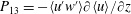 $P_{13}=-\langle u^{\prime }w^{\prime }\rangle \unicode[STIX]{x2202}\langle u\rangle /\unicode[STIX]{x2202}z$
is large in the region between the stagnation point S1 and the core of vortex V1 (figure 16
d). In this region, the streamlines in figure 7 bear large curvature and there is a large shear rate in the streamwise velocity component. The location of its maximum corresponds approximately to the peak position of
$P_{13}=-\langle u^{\prime }w^{\prime }\rangle \unicode[STIX]{x2202}\langle u\rangle /\unicode[STIX]{x2202}z$
is large in the region between the stagnation point S1 and the core of vortex V1 (figure 16
d). In this region, the streamlines in figure 7 bear large curvature and there is a large shear rate in the streamwise velocity component. The location of its maximum corresponds approximately to the peak position of
 $-\langle u^{\prime }w^{\prime }\rangle$
(figure 13). This patch of positive shear production is a main contributor to the total production of turbulent kinetic energy, which becomes evident when comparing with figure 15.
$-\langle u^{\prime }w^{\prime }\rangle$
(figure 13). This patch of positive shear production is a main contributor to the total production of turbulent kinetic energy, which becomes evident when comparing with figure 15.
Negative shear production can be found in three regions. The first region lies close to the wall between the streamwise positions of S1 and V1. This peak can be explained by the wall-normal gradient of
 $\langle u\rangle$
in the wall jet. Above the velocity maximum in the jet, the gradient is negative
$\langle u\rangle$
in the wall jet. Above the velocity maximum in the jet, the gradient is negative
 $\unicode[STIX]{x2202}\langle u\rangle /\unicode[STIX]{x2202}z<0$
. Below the maximum, it is positive. As
$\unicode[STIX]{x2202}\langle u\rangle /\unicode[STIX]{x2202}z<0$
. Below the maximum, it is positive. As
 $\langle u^{\prime }w^{\prime }\rangle$
is negative in the whole region, the production changes sign and becomes negative in the lower part of the jet. The fact that the Reynolds shear stress does not change sign when the velocity gradient changes sign indicates that large-scale fluctuations penetrate this jet and reach the wall.
$\langle u^{\prime }w^{\prime }\rangle$
is negative in the whole region, the production changes sign and becomes negative in the lower part of the jet. The fact that the Reynolds shear stress does not change sign when the velocity gradient changes sign indicates that large-scale fluctuations penetrate this jet and reach the wall.
The second location in which negative shear production can be found is in the upper right part of the main vortex V1 (
 $x/D\approx -0.7$
), in which free-stream fluid is entrained into the vortex. The streamlines are pointing downwards and in the direction of the cylinder. Like in the other regions of the horseshoe vortex, the streamwise velocity has a positive vertical gradient
$x/D\approx -0.7$
), in which free-stream fluid is entrained into the vortex. The streamlines are pointing downwards and in the direction of the cylinder. Like in the other regions of the horseshoe vortex, the streamwise velocity has a positive vertical gradient
 $\unicode[STIX]{x2202}\langle u\rangle /\unicode[STIX]{x2202}z>0$
. We find positive
$\unicode[STIX]{x2202}\langle u\rangle /\unicode[STIX]{x2202}z>0$
. We find positive
 $\langle u^{\prime }w^{\prime }\rangle$
in this region (figure 13). Together, this gives a negative shear production of turbulent kinetic energy at a significant level. The third location with negative
$\langle u^{\prime }w^{\prime }\rangle$
in this region (figure 13). Together, this gives a negative shear production of turbulent kinetic energy at a significant level. The third location with negative
 $P_{13}$
is a large area in front of the cylinder for
$P_{13}$
is a large area in front of the cylinder for
 $x/D\gtrsim -0.6$
. The magnitude is small but noticeable. Around vortex V3, however, we can see significant positive values of shear production. We do not show
$x/D\gtrsim -0.6$
. The magnitude is small but noticeable. Around vortex V3, however, we can see significant positive values of shear production. We do not show
 $P_{31}$
as its amplitude is approximately one order of magnitude smaller than that of the other terms.
$P_{31}$
as its amplitude is approximately one order of magnitude smaller than that of the other terms.

Figure 17. Isosurfaces of the total production of turbulent kinetic energy
 $P$
around the cylinder:
$P$
around the cylinder:
 $PD/u_{b}^{3}=-0.02$
(blue),
$PD/u_{b}^{3}=-0.02$
(blue),
 $PD/u_{b}^{3}=0.1$
(red) and
$PD/u_{b}^{3}=0.1$
(red) and
 $PD/u_{b}^{3}=0.25$
(green) are evaluated from the LES. The isosurface for
$PD/u_{b}^{3}=0.25$
(green) are evaluated from the LES. The isosurface for
 $PD/u_{b}^{3}=0.1$
is only shown up to the symmetry plane.
$PD/u_{b}^{3}=0.1$
is only shown up to the symmetry plane.
To gain insight into the three-dimensional distribution of production in front of the cylinder, isosurfaces of
 $P$
are evaluated in figure 17. The isovalues have been chosen to be representative for specific regions of production, as explained in the following. The red isosurface marks values of
$P$
are evaluated in figure 17. The isovalues have been chosen to be representative for specific regions of production, as explained in the following. The red isosurface marks values of
 $PD/u_{b}^{3}=0.1$
and surrounds the regions in which medium production takes place. Its cross-section has the distinct c-shape typical for the distribution of
$PD/u_{b}^{3}=0.1$
and surrounds the regions in which medium production takes place. Its cross-section has the distinct c-shape typical for the distribution of
 $k$
. The isosurface
$k$
. The isosurface
 $PD/u_{b}^{3}=0.25$
visualizes the two regions of largest production, which are not connected – one is approximately in the position of the vortex core of V1 and the other one is where the leg of the c-shape meets the bottom plate. It should be noted that the green isosurface in the vortex core ends at an angle of approximately
$PD/u_{b}^{3}=0.25$
visualizes the two regions of largest production, which are not connected – one is approximately in the position of the vortex core of V1 and the other one is where the leg of the c-shape meets the bottom plate. It should be noted that the green isosurface in the vortex core ends at an angle of approximately
 $45^{\circ }$
to the symmetry plane, while the green region at the bottom plate wraps around the cylinder to an angle of approximately
$45^{\circ }$
to the symmetry plane, while the green region at the bottom plate wraps around the cylinder to an angle of approximately
 $90^{\circ }$
.
$90^{\circ }$
.
In front of the cylinder at the bottom plate, there is a large region of turbulent kinetic energy destruction, i.e. negative production; see the blue isosurface
 $PD/u_{b}^{3}=-0.02$
in figure 17. This is the region in which the upstream-directed jet along the bottom plate accelerates, leading to negative normal stress production. This negative normal stress production can be found all around the cylinder until approximately
$PD/u_{b}^{3}=-0.02$
in figure 17. This is the region in which the upstream-directed jet along the bottom plate accelerates, leading to negative normal stress production. This negative normal stress production can be found all around the cylinder until approximately
 $90^{\circ }$
. It can explain the low level of turbulent kinetic energy between the cylinder and V1 which extends half way round the cylinder (compare figures 12 and 14).
$90^{\circ }$
. It can explain the low level of turbulent kinetic energy between the cylinder and V1 which extends half way round the cylinder (compare figures 12 and 14).
It should be mentioned that the disturbances of the isosurfaces in the lateral front of the cylinder are artefacts stemming from the numerical scheme. It should be noted that second-order central approximations favour wiggles in strong curvature regions when the cell Reynolds number exceeds a value of 2.0. This is the case here, and we do not intend to damp these wiggles as they indicate an insufficient grid resolution (Gresho & Lee Reference Gresho and Lee1981) and have only marginal effects on the flow dynamics in the symmetry plane which is the focus of the present investigation.
6.4 Dissipation
In this section, we discuss the dissipation
 $\unicode[STIX]{x1D716}$
of turbulent kinetic energy (6.7). The distribution and level of dissipation are of relevance to turbulence modelling in the Reynolds-averaged context. In a flow with local equilibrium, the dissipation would be equal to the production of turbulent kinetic energy. Since local equilibrium cannot be expected in the considered flow, we cannot expect the spatial distribution of the dissipation of turbulent kinetic energy to match the distribution of its production.
$\unicode[STIX]{x1D716}$
of turbulent kinetic energy (6.7). The distribution and level of dissipation are of relevance to turbulence modelling in the Reynolds-averaged context. In a flow with local equilibrium, the dissipation would be equal to the production of turbulent kinetic energy. Since local equilibrium cannot be expected in the considered flow, we cannot expect the spatial distribution of the dissipation of turbulent kinetic energy to match the distribution of its production.
The dissipation rates in the symmetry plane in the cylinder front as obtained from PIV and LES are presented in figure 18. Large values of
 $\unicode[STIX]{x1D716}$
can be observed around the core of vortex V1. A second peak is placed right beneath in the leg of the c-shape of the turbulent kinetic energy distribution, where the jet decelerates. A third peak is located in the region of the corner vortex V3. The LES data in figure 18(b) show significant levels of dissipation along the bottom plate, where the jet is causing large shear stresses. This stripe of large
$\unicode[STIX]{x1D716}$
can be observed around the core of vortex V1. A second peak is placed right beneath in the leg of the c-shape of the turbulent kinetic energy distribution, where the jet decelerates. A third peak is located in the region of the corner vortex V3. The LES data in figure 18(b) show significant levels of dissipation along the bottom plate, where the jet is causing large shear stresses. This stripe of large
 $\unicode[STIX]{x1D716}$
is not visible in the PIV data since the standard PIV algorithm, which has been applied to compute the dissipation terms, does not resolve the wall in a sufficient way.
$\unicode[STIX]{x1D716}$
is not visible in the PIV data since the standard PIV algorithm, which has been applied to compute the dissipation terms, does not resolve the wall in a sufficient way.

Figure 18. The total dissipation of turbulent kinetic energy
 $\unicode[STIX]{x1D716}D/u_{b}^{3}$
taken from PIV (a) and LES (b), and the modelled dissipation
$\unicode[STIX]{x1D716}D/u_{b}^{3}$
taken from PIV (a) and LES (b), and the modelled dissipation
 $\unicode[STIX]{x1D716}_{SGS}D/u_{b}^{3}$
taken from LES (c) in the symmetry plane in front of the cylinder. The different amplitudes of the colour bars should be noted.
$\unicode[STIX]{x1D716}_{SGS}D/u_{b}^{3}$
taken from LES (c) in the symmetry plane in front of the cylinder. The different amplitudes of the colour bars should be noted.
The spatial distribution of the dissipation does in fact largely resemble the distribution of the turbulent kinetic energy in figure 12. The peaks of both the turbulent kinetic energy and its dissipation are shifted in space with respect to the ones of the production (figure 15). In the measured distribution, the peak of
 $\unicode[STIX]{x1D716}$
is downstream of the vortex core V1. The streamlines reaching this location stem from the approach flow, which indicates that the dissipative scales reaching the location of the dissipation peak cannot be transported to this location by the time-averaged flow field. We speculate that the bimodal oscillations of the horseshoe vortex give rise to turbulent transport of small-scale structures from the locations of large turbulent kinetic energy production to the locations where they are dissipated. This process would lead to large magnitudes of the turbulent transport terms
$\unicode[STIX]{x1D716}$
is downstream of the vortex core V1. The streamlines reaching this location stem from the approach flow, which indicates that the dissipative scales reaching the location of the dissipation peak cannot be transported to this location by the time-averaged flow field. We speculate that the bimodal oscillations of the horseshoe vortex give rise to turbulent transport of small-scale structures from the locations of large turbulent kinetic energy production to the locations where they are dissipated. This process would lead to large magnitudes of the turbulent transport terms
 $T_{conv}$
and
$T_{conv}$
and
 $T_{pres}$
. We discuss this hypothesis in the following sections.
$T_{pres}$
. We discuss this hypothesis in the following sections.
The dissipation rate from PIV shown in figure 18(a) is computed from in-plane velocity gradients only, while the one from LES is computed from the full tensor including subgrid contributions (6.7). Nevertheless, the measured dissipation rate is larger by a factor of approximately 1.7. This factor is in compliance with the larger levels of turbulent kinetic energy and its production in the experiment. However, it needs to be taken with caution as in the experimental values only the in-plane gradients of the in-plane velocity components have been taken into account. The full dissipation would have larger values. It is known that an estimation of the dissipation rate from PIV data suffers from two sources of error. If the interrogation windows are considerably larger than the Kolmogorov scale, the dissipation will be underestimated. If the interrogation window is in the range of or smaller than the Kolmogorov scale, it can be overestimated by measurement noise (Tanaka & Eaton Reference Tanaka and Eaton2007). It should be noted that we did not apply any correction to our PIV results to account for the noise or insufficient resolution as we did not know the value and distribution of the Kolmogorov scale in advance.
It is natural to assume that the LES is not able to resolve the small dissipative structures of the flow. However, we have to stress that the dissipation taken from the LES includes the modelled dissipation
 $\unicode[STIX]{x1D716}_{SGS}$
. The latter is documented in figure 18(c). In the region of V1,
$\unicode[STIX]{x1D716}_{SGS}$
. The latter is documented in figure 18(c). In the region of V1,
 $\unicode[STIX]{x1D716}_{SGS}$
is approximately one third of the total dissipation. This is a perceptible contribution. However, the amplitude of
$\unicode[STIX]{x1D716}_{SGS}$
is approximately one third of the total dissipation. This is a perceptible contribution. However, the amplitude of
 $\unicode[STIX]{x1D716}_{SGS}$
is too small to assign the difference in amplitudes of PIV and LES to possible shortcomings of the subgrid stress model. We keep the discussion on the level of the dissipation rate for later when the whole budget is discussed.
$\unicode[STIX]{x1D716}_{SGS}$
is too small to assign the difference in amplitudes of PIV and LES to possible shortcomings of the subgrid stress model. We keep the discussion on the level of the dissipation rate for later when the whole budget is discussed.
To further study the characteristics of the turbulence structure, the pseudo dissipation
 $\unicode[STIX]{x1D716}_{p}=\unicode[STIX]{x1D708}\langle (\unicode[STIX]{x2202}u_{i}^{\prime }/\unicode[STIX]{x2202}x_{j})^{2}\rangle$
(Schlichting & Gersten Reference Schlichting and Gersten2006) was investigated. A comparison of the pseudo dissipation
$\unicode[STIX]{x1D716}_{p}=\unicode[STIX]{x1D708}\langle (\unicode[STIX]{x2202}u_{i}^{\prime }/\unicode[STIX]{x2202}x_{j})^{2}\rangle$
(Schlichting & Gersten Reference Schlichting and Gersten2006) was investigated. A comparison of the pseudo dissipation
 $\unicode[STIX]{x1D716}_{p}$
with the dissipation
$\unicode[STIX]{x1D716}_{p}$
with the dissipation
 $\unicode[STIX]{x1D716}$
, both taken from the LES, shows only marginal differences. Therefore, a detailed discussion of the complete
$\unicode[STIX]{x1D716}$
, both taken from the LES, shows only marginal differences. Therefore, a detailed discussion of the complete
 $\unicode[STIX]{x1D716}_{p}$
is omitted here. Nevertheless, the structure of
$\unicode[STIX]{x1D716}_{p}$
is omitted here. Nevertheless, the structure of
 $\unicode[STIX]{x1D716}_{p}$
allows us to decompose the pseudo dissipation into dissipation by the streamwise fluctuations
$\unicode[STIX]{x1D716}_{p}$
allows us to decompose the pseudo dissipation into dissipation by the streamwise fluctuations
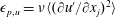 $\unicode[STIX]{x1D716}_{p,u}=\unicode[STIX]{x1D708}\langle (\unicode[STIX]{x2202}u^{\prime }/\unicode[STIX]{x2202}x_{j})^{2}\rangle$
, the spanwise fluctuations
$\unicode[STIX]{x1D716}_{p,u}=\unicode[STIX]{x1D708}\langle (\unicode[STIX]{x2202}u^{\prime }/\unicode[STIX]{x2202}x_{j})^{2}\rangle$
, the spanwise fluctuations
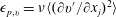 $\unicode[STIX]{x1D716}_{p,v}=\unicode[STIX]{x1D708}\langle (\unicode[STIX]{x2202}v^{\prime }/\unicode[STIX]{x2202}x_{j})^{2}\rangle$
and the vertical fluctuations
$\unicode[STIX]{x1D716}_{p,v}=\unicode[STIX]{x1D708}\langle (\unicode[STIX]{x2202}v^{\prime }/\unicode[STIX]{x2202}x_{j})^{2}\rangle$
and the vertical fluctuations
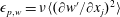 $\unicode[STIX]{x1D716}_{p,w}=\unicode[STIX]{x1D708}\langle (\unicode[STIX]{x2202}w^{\prime }/\unicode[STIX]{x2202}x_{j})^{2}\rangle$
. The resulting distributions are shown in figure 19.
$\unicode[STIX]{x1D716}_{p,w}=\unicode[STIX]{x1D708}\langle (\unicode[STIX]{x2202}w^{\prime }/\unicode[STIX]{x2202}x_{j})^{2}\rangle$
. The resulting distributions are shown in figure 19.

Figure 19. Components of the pseudo dissipation in the symmetry plane in front of the cylinder:
 $\unicode[STIX]{x1D716}_{p,u}D/u_{b}^{3}$
in the streamwise (a),
$\unicode[STIX]{x1D716}_{p,u}D/u_{b}^{3}$
in the streamwise (a),
 $\unicode[STIX]{x1D716}_{p,v}D/u_{b}^{3}$
in the spanwise (b) and
$\unicode[STIX]{x1D716}_{p,v}D/u_{b}^{3}$
in the spanwise (b) and
 $\unicode[STIX]{x1D716}_{p,w}D/u_{b}^{3}$
in the vertical direction (c), taken from the LES.
$\unicode[STIX]{x1D716}_{p,w}D/u_{b}^{3}$
in the vertical direction (c), taken from the LES.
In the region of the main vortex V1, the single components of
 $\unicode[STIX]{x1D716}_{p}$
look almost the same. This is true for the distributions as well as the amplitudes and suggests that the small-scale turbulence is isotropic here. Along the bottom wall,
$\unicode[STIX]{x1D716}_{p}$
look almost the same. This is true for the distributions as well as the amplitudes and suggests that the small-scale turbulence is isotropic here. Along the bottom wall,
 $\unicode[STIX]{x1D716}_{p,u}$
is the dominant contributor to the pseudo dissipation. This is especially true for the deceleration zone of the wall jet, where
$\unicode[STIX]{x1D716}_{p,u}$
is the dominant contributor to the pseudo dissipation. This is especially true for the deceleration zone of the wall jet, where
 $\unicode[STIX]{x1D716}_{p,u}$
reaches its maximum of up to
$\unicode[STIX]{x1D716}_{p,u}$
reaches its maximum of up to
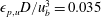 $\unicode[STIX]{x1D716}_{p,u}D/u_{b}^{3}=0.035$
. Further splitting of
$\unicode[STIX]{x1D716}_{p,u}D/u_{b}^{3}=0.035$
. Further splitting of
 $\unicode[STIX]{x1D716}_{p,u}$
reveals
$\unicode[STIX]{x1D716}_{p,u}$
reveals
 $\langle (\unicode[STIX]{x2202}u^{\prime }/\unicode[STIX]{x2202}z)^{2}\rangle$
to be the main contributor here, while the other two contributions
$\langle (\unicode[STIX]{x2202}u^{\prime }/\unicode[STIX]{x2202}z)^{2}\rangle$
to be the main contributor here, while the other two contributions
 $\langle (\unicode[STIX]{x2202}u^{\prime }/\unicode[STIX]{x2202}x)^{2}\rangle$
and
$\langle (\unicode[STIX]{x2202}u^{\prime }/\unicode[STIX]{x2202}x)^{2}\rangle$
and
 $\langle (\unicode[STIX]{x2202}u^{\prime }/\unicode[STIX]{x2202}y)^{2}\rangle$
are almost zero. This indicates that a vertical flapping of the wall jet is the main source of turbulent dissipation (and fluctuations) in this region.
$\langle (\unicode[STIX]{x2202}u^{\prime }/\unicode[STIX]{x2202}y)^{2}\rangle$
are almost zero. This indicates that a vertical flapping of the wall jet is the main source of turbulent dissipation (and fluctuations) in this region.
Along the flow-facing edge of the cylinder,
 $\unicode[STIX]{x1D716}_{p,w}$
dominates the pseudo dissipation. There is a thin layer of large
$\unicode[STIX]{x1D716}_{p,w}$
dominates the pseudo dissipation. There is a thin layer of large
 $\unicode[STIX]{x1D716}_{p,w}$
along the cylinder front, stretching into the region covered by V3. Nevertheless, for
$\unicode[STIX]{x1D716}_{p,w}$
along the cylinder front, stretching into the region covered by V3. Nevertheless, for
 $z<0.07D$
,
$z<0.07D$
,
 $\unicode[STIX]{x1D716}_{p,u}$
and
$\unicode[STIX]{x1D716}_{p,u}$
and
 $\unicode[STIX]{x1D716}_{p,v}$
also give significant contributions.
$\unicode[STIX]{x1D716}_{p,v}$
also give significant contributions.
The maximum levels of dissipation reached in the horseshoe vortex are considerably lower than what a macroscale estimation
 $\unicode[STIX]{x1D716}_{macro}=u_{b}^{3}/D$
(Pope Reference Pope2011) gives. Estimation of the Kolmogorov length scale
$\unicode[STIX]{x1D716}_{macro}=u_{b}^{3}/D$
(Pope Reference Pope2011) gives. Estimation of the Kolmogorov length scale
 $\unicode[STIX]{x1D702}_{K}=(\unicode[STIX]{x1D708}^{3}/\unicode[STIX]{x1D716})^{1/4}$
(Pope Reference Pope2011) in the core of the horseshoe vortex based on
$\unicode[STIX]{x1D702}_{K}=(\unicode[STIX]{x1D708}^{3}/\unicode[STIX]{x1D716})^{1/4}$
(Pope Reference Pope2011) in the core of the horseshoe vortex based on
 $\unicode[STIX]{x1D716}_{macro}$
gives
$\unicode[STIX]{x1D716}_{macro}$
gives
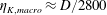 $\unicode[STIX]{x1D702}_{K,macro}\approx D/2800$
. Insertion of the PIV measurement
$\unicode[STIX]{x1D702}_{K,macro}\approx D/2800$
. Insertion of the PIV measurement
 $\unicode[STIX]{x1D716}_{PIV}$
gives
$\unicode[STIX]{x1D716}_{PIV}$
gives
 $\unicode[STIX]{x1D702}_{K,PIV}\approx D/1600$
, and the dissipation taken from the LES results in a Kolmogorov length scale of
$\unicode[STIX]{x1D702}_{K,PIV}\approx D/1600$
, and the dissipation taken from the LES results in a Kolmogorov length scale of
 $\unicode[STIX]{x1D702}_{K,LES}\approx D/1500$
. Using the estimation of Pope (Reference Pope2011) for the required grid resolution in a direct numerical simulation (DNS),
$\unicode[STIX]{x1D702}_{K,LES}\approx D/1500$
. Using the estimation of Pope (Reference Pope2011) for the required grid resolution in a direct numerical simulation (DNS),
 $\unicode[STIX]{x0394}x_{i}\lesssim 2\unicode[STIX]{x1D702}_{K}$
, we can conclude that our wall-normal grid resolution would be sufficient for a DNS. On the other hand, our horizontal resolutions are marginally too coarse, which is consistent with a noticeable fraction of modelled dissipation.
$\unicode[STIX]{x0394}x_{i}\lesssim 2\unicode[STIX]{x1D702}_{K}$
, we can conclude that our wall-normal grid resolution would be sufficient for a DNS. On the other hand, our horizontal resolutions are marginally too coarse, which is consistent with a noticeable fraction of modelled dissipation.
6.5 Turbulent transport of turbulent kinetic energy
In non-equilibrium flow situations such as the considered one, the turbulent kinetic energy needs to be redistributed in space by the convection by the mean velocity field
 $C$
(6.2) and the turbulent transport terms, namely the turbulent convection
$C$
(6.2) and the turbulent transport terms, namely the turbulent convection
 $T_{conv}$
, the pressure transport
$T_{conv}$
, the pressure transport
 $T_{pres}$
and the viscous diffusion
$T_{pres}$
and the viscous diffusion
 $T_{visc}$
(6.3)–(6.5). This subsection concentrates on the turbulent transport mechanisms. The convection by the mean mainly documents whether the turbulent kinetic energy was increasing (negative convection) or decreasing (positive convection) along a streamline. We omit a discussion of its spatial distribution, just pointing out that the main increase of turbulent kinetic energy along a streamline occurs in the deceleration region of the jet under the horseshoe vortex where the streamwise fluctuations are produced. The viscous diffusion term has a significantly smaller amplitude than the other redistribution terms. We therefore omit its discussion as well.
$T_{visc}$
(6.3)–(6.5). This subsection concentrates on the turbulent transport mechanisms. The convection by the mean mainly documents whether the turbulent kinetic energy was increasing (negative convection) or decreasing (positive convection) along a streamline. We omit a discussion of its spatial distribution, just pointing out that the main increase of turbulent kinetic energy along a streamline occurs in the deceleration region of the jet under the horseshoe vortex where the streamwise fluctuations are produced. The viscous diffusion term has a significantly smaller amplitude than the other redistribution terms. We therefore omit its discussion as well.

Figure 20. Turbulent convection
 $T_{conv}D/u_{b}^{3}$
(a) and pressure transport
$T_{conv}D/u_{b}^{3}$
(a) and pressure transport
 $T_{pres}D/u_{b}^{3}$
(b) taken from the LES.
$T_{pres}D/u_{b}^{3}$
(b) taken from the LES.
Figure 20 illustrates the turbulent transport terms from LES. There is no noticeable difference between the full and in-plane turbulent convection in the LES results, which indicates out-of-plane turbulent convection to be insignificant in the symmetry plane in front of the cylinder. The distribution of the turbulent convection
 $T_{conv}$
(figure 20
a) is similar to the production term illustrated in figure 15. In regions in which large production of turbulent kinetic energy takes place, we see large negative turbulent convection. There are regions, e.g. close to the wall at
$T_{conv}$
(figure 20
a) is similar to the production term illustrated in figure 15. In regions in which large production of turbulent kinetic energy takes place, we see large negative turbulent convection. There are regions, e.g. close to the wall at
 $x/D=-0.75$
, in which the production rate is nearly balanced by turbulent convection. In these areas, the turbulence is characterized by violent eruptions, which might quickly sweep the turbulent fluctuations to another place. This interpretation is in line with what Apsilidis et al. (Reference Apsilidis, Diplas, Dancey and Bouratsis2015) describe when discussing instantaneous flow fields.
$x/D=-0.75$
, in which the production rate is nearly balanced by turbulent convection. In these areas, the turbulence is characterized by violent eruptions, which might quickly sweep the turbulent fluctuations to another place. This interpretation is in line with what Apsilidis et al. (Reference Apsilidis, Diplas, Dancey and Bouratsis2015) describe when discussing instantaneous flow fields.
The distribution of
 $\langle p^{\prime 2}\rangle$
(not shown) implies that the core of the main vortex V1 bounces between
$\langle p^{\prime 2}\rangle$
(not shown) implies that the core of the main vortex V1 bounces between
 $x=-0.78D$
and
$x=-0.78D$
and
 $x=-0.66D$
due to its bimodality, leading to large pressure fluctuations at these positions. These fluctuations result in the two peaks of large negative
$x=-0.66D$
due to its bimodality, leading to large pressure fluctuations at these positions. These fluctuations result in the two peaks of large negative
 $T_{pres}$
in figure 20(b), which are located approximately at the upstream and downstream ends of the mentioned range. In addition, there is a peak of positive pressure transport right underneath V1 at
$T_{pres}$
in figure 20(b), which are located approximately at the upstream and downstream ends of the mentioned range. In addition, there is a peak of positive pressure transport right underneath V1 at
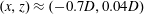 $(x,z)\approx (-0.7D,0.04D)$
. This spot has a branch reaching to the bottom plate.
$(x,z)\approx (-0.7D,0.04D)$
. This spot has a branch reaching to the bottom plate.
In some regions, the pressure transport has the opposite sign to the turbulent convection and a similar magnitude,
 $T_{pres}\approx -T_{conv}$
. This implies that for a large part of the time,
$T_{pres}\approx -T_{conv}$
. This implies that for a large part of the time,
 $p^{\prime }\approx -0.5\unicode[STIX]{x1D70C}u_{i}^{\prime }u_{i}^{\prime }$
(compare (6.3) and (6.4)). This can be observed at approximately
$p^{\prime }\approx -0.5\unicode[STIX]{x1D70C}u_{i}^{\prime }u_{i}^{\prime }$
(compare (6.3) and (6.4)). This can be observed at approximately
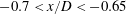 $-0.7<x/D<-0.65$
, slightly below and above V1. In these regions, the two terms
$-0.7<x/D<-0.65$
, slightly below and above V1. In these regions, the two terms
 $T_{conv}$
and
$T_{conv}$
and
 $T_{pres}$
seem to cancel each other. We can explain such behaviour by horizontal oscillations of the horseshoe vortex V1. If this vortex is shifted downstream, e.g. from its mean position at
$T_{pres}$
seem to cancel each other. We can explain such behaviour by horizontal oscillations of the horseshoe vortex V1. If this vortex is shifted downstream, e.g. from its mean position at
 $x/D=-0.73$
to approximately
$x/D=-0.73$
to approximately
 $x/D=-0.68$
, the vortex core is in a position in which the time-averaged flow has a large negative wall-normal component. The instantaneous vertical velocity in the vortex core is zero, which gives rise to a positive wall-normal fluctuation
$x/D=-0.68$
, the vortex core is in a position in which the time-averaged flow has a large negative wall-normal component. The instantaneous vertical velocity in the vortex core is zero, which gives rise to a positive wall-normal fluctuation
 $w^{\prime }>0$
. As
$w^{\prime }>0$
. As
 $u_{j}^{\prime }u_{j}^{\prime }$
is positive as well, the triple correlation
$u_{j}^{\prime }u_{j}^{\prime }$
is positive as well, the triple correlation
 $\langle u_{i}^{\prime }u_{j}^{\prime }u_{j}^{\prime }\rangle$
will obtain a strong positive contribution. As the convective term is the negative gradient of the triple correlation, this situation will give rise to a large negative contribution to
$\langle u_{i}^{\prime }u_{j}^{\prime }u_{j}^{\prime }\rangle$
will obtain a strong positive contribution. As the convective term is the negative gradient of the triple correlation, this situation will give rise to a large negative contribution to
 $T_{conv}$
under the vortex core and a large positive contribution above the vortex core. It can be assumed that
$T_{conv}$
under the vortex core and a large positive contribution above the vortex core. It can be assumed that
 $p^{\prime }<0$
in the vortex core, giving rise to a
$p^{\prime }<0$
in the vortex core, giving rise to a
 $T_{pres}$
that has the opposite sign to
$T_{pres}$
that has the opposite sign to
 $T_{conv}$
.
$T_{conv}$
.
6.6 Balance of turbulent kinetic energy
To further assess the interplay of the previously discussed mechanisms, we discuss the complete balance of turbulent kinetic energy (6.1) along two horizontal lines through the vortex system.

Figure 21. The budget of the turbulent kinetic energy in the cylinder front from LES at a wall distance of
 $z/D=0.012$
(a) and
$z/D=0.012$
(a) and
 $z/D=0.065$
(b). For reasons of visibility, only every second data point is plotted. The vertical lines indicate the position of V1. All values are normalized by
$z/D=0.065$
(b). For reasons of visibility, only every second data point is plotted. The vertical lines indicate the position of V1. All values are normalized by
 $D/u_{b}^{3}$
.
$D/u_{b}^{3}$
.
Figure 21(a) shows profiles of each term of (6.1) along a horizontal line with a wall distance of
 $z/D=0.012$
, which is inside the near-wall jet. The distribution along the horizontal line can be divided into four parts. Starting from the cylinder, we first identify the vortex V3, giving rise to large production magnitudes balanced locally in parts by dissipation. Turbulent convection and convection by the mean velocity field also play a role in this region as well as pressure transport.
$z/D=0.012$
, which is inside the near-wall jet. The distribution along the horizontal line can be divided into four parts. Starting from the cylinder, we first identify the vortex V3, giving rise to large production magnitudes balanced locally in parts by dissipation. Turbulent convection and convection by the mean velocity field also play a role in this region as well as pressure transport.
The zone between V3 and the deceleration of the jet (
 $-0.55<x/D<-0.68$
) is characterized by nearly zero or even negative production rates. However, we see that the convection by the mean is negative, which means that the turbulent kinetic energy increases along the streamlines. The budget is closed here only if the pressure transport term is included in the balance. This is the only positive term that transports turbulent kinetic energy into the calm zone in front of the cylinder where the downflow turns upstream and accelerates. This pressure transport is balanced by negative production around
$-0.55<x/D<-0.68$
) is characterized by nearly zero or even negative production rates. However, we see that the convection by the mean is negative, which means that the turbulent kinetic energy increases along the streamlines. The budget is closed here only if the pressure transport term is included in the balance. This is the only positive term that transports turbulent kinetic energy into the calm zone in front of the cylinder where the downflow turns upstream and accelerates. This pressure transport is balanced by negative production around
 $x/D=0.58$
and by mean convection and dissipation further upstream.
$x/D=0.58$
and by mean convection and dissipation further upstream.
When the jet decelerates under the horseshoe vortex, a large amount of production takes place, which has been shown to occur predominantly in the streamwise component. The large negative amplitude of the mean convection term at
 $x/D\approx 0.72$
indicates that the turbulent kinetic energy rises strongly along the streamlines. This is because the dissipation remains much smaller than the production and the other transport terms remain small or are even positive, such as the pressure transport. Around the peak value of the production term, the mean convection crosses zero, which indicates that this is also the peak of the turbulent kinetic energy. Upstream of this point, the turbulent convection is negative and has larger magnitudes than the production, which leads to a decrease of turbulent kinetic energy along a streamline, as indicated by positive mean convection.
$x/D\approx 0.72$
indicates that the turbulent kinetic energy rises strongly along the streamlines. This is because the dissipation remains much smaller than the production and the other transport terms remain small or are even positive, such as the pressure transport. Around the peak value of the production term, the mean convection crosses zero, which indicates that this is also the peak of the turbulent kinetic energy. Upstream of this point, the turbulent convection is negative and has larger magnitudes than the production, which leads to a decrease of turbulent kinetic energy along a streamline, as indicated by positive mean convection.
Horizontal profiles of all budget terms at a larger wall distance,
 $z/D=0.065$
, are shown in figure 21(b). This is the wall distance of the vortex core V1. As in the near-wall profiles, there are four regions in which the behaviour of the budget terms differs. On moving upstream from the cylinder, there is the near-cylinder downflow in which locally turbulent kinetic energy is produced. Unfortunately, this layer is not well resolved by the LES and the values do not seem realistic, which is underlined by a large residual of the budget in the wall-nearest point.
$z/D=0.065$
, are shown in figure 21(b). This is the wall distance of the vortex core V1. As in the near-wall profiles, there are four regions in which the behaviour of the budget terms differs. On moving upstream from the cylinder, there is the near-cylinder downflow in which locally turbulent kinetic energy is produced. Unfortunately, this layer is not well resolved by the LES and the values do not seem realistic, which is underlined by a large residual of the budget in the wall-nearest point.
Moving upstream from the cylinder in the region
 $x/D>-0.65$
, we see small values of all budget terms. This is the downflow region. However, at
$x/D>-0.65$
, we see small values of all budget terms. This is the downflow region. However, at
 $x/D<-0.65$
, there is a sudden rise in the levels of turbulent convection and pressure transport. This is the zone in which the turbulent convection approximately balances the pressure transport. We conjecture that this behaviour could be explained by a periodical horizontal displacement of the horseshoe vortex V1 to locations around
$x/D<-0.65$
, there is a sudden rise in the levels of turbulent convection and pressure transport. This is the zone in which the turbulent convection approximately balances the pressure transport. We conjecture that this behaviour could be explained by a periodical horizontal displacement of the horseshoe vortex V1 to locations around
 $x/D=-0.68$
.
$x/D=-0.68$
.
The production of turbulent kinetic energy has a broad peak slightly upstream of V1. The production is mainly balanced by dissipation and turbulent convection in this zone (
 $x/D\approx -0.8$
). Turbulent convection seems to bring turbulent kinetic energy upstream and downstream from the production peak. Upstream of the production peak, the turbulent convection is positive and adds to the production, while both together seem to be balanced by the mean convection and small but noticeable dissipation.
$x/D\approx -0.8$
). Turbulent convection seems to bring turbulent kinetic energy upstream and downstream from the production peak. Upstream of the production peak, the turbulent convection is positive and adds to the production, while both together seem to be balanced by the mean convection and small but noticeable dissipation.
The budget evaluated by the LES including all terms of (6.1) sums up to zero in a satisfying way (figure 22). In the large grey regions in figure 22, the amplitude of the budget residual
 $R$
is
$R$
is
 $|R|=|C+T_{conv}+T_{pres}+T_{visc}+P-\unicode[STIX]{x1D716}|<0.01u_{b}^{3}/D$
. Regions coloured by slightly lighter or slightly darker grey indicate
$|R|=|C+T_{conv}+T_{pres}+T_{visc}+P-\unicode[STIX]{x1D716}|<0.01u_{b}^{3}/D$
. Regions coloured by slightly lighter or slightly darker grey indicate
 $|R|D/u_{b}^{3}<0.03$
, which remains below 10 % of the production term. Small spots close to the cylinder front and along the bottom plate show values of
$|R|D/u_{b}^{3}<0.03$
, which remains below 10 % of the production term. Small spots close to the cylinder front and along the bottom plate show values of
 $|R|D/u_{b}^{3}<0.3$
. We suspect that the reason for these large errors along the cylinder front is the grid resolution in the horizontal direction, which is four times larger than the vertical one. Thus, the boundary layer along the cylinder cannot be considered to be wall-resolved, resulting in inaccuracies in this limited region. Furthermore, subgrid contributors are not included in the evaluation of the discussed terms except for the dissipation. As figure 5 implies, the contribution of the subgrid stresses is considerable in narrow regions around vortex V3. This further explains the large residual here.
$|R|D/u_{b}^{3}<0.3$
. We suspect that the reason for these large errors along the cylinder front is the grid resolution in the horizontal direction, which is four times larger than the vertical one. Thus, the boundary layer along the cylinder cannot be considered to be wall-resolved, resulting in inaccuracies in this limited region. Furthermore, subgrid contributors are not included in the evaluation of the discussed terms except for the dissipation. As figure 5 implies, the contribution of the subgrid stresses is considerable in narrow regions around vortex V3. This further explains the large residual here.

Figure 22. The budget residual
 $RD/u_{b}^{3}$
in the cylinder front taken from the LES.
$RD/u_{b}^{3}$
in the cylinder front taken from the LES.
Large errors along the bottom plate in the first line appear where the amplitude of the turbulent convection
 $T_{conv}$
is large. The triple correlations necessary to evaluate
$T_{conv}$
is large. The triple correlations necessary to evaluate
 $T_{conv}$
are sensitive to statistical errors and need a large number of samples to converge. Thus, statistics that are not fully converged might be a reason for this large error amplitude here as well. The fact that the residual has positive and negative values is an indication that the level of dissipation predicted by the LES is realistic. As the out-of-plane terms and the pressure transport are missing in the PIV data, we did not make any attempt to compute the total balance for the PIV data.
$T_{conv}$
are sensitive to statistical errors and need a large number of samples to converge. Thus, statistics that are not fully converged might be a reason for this large error amplitude here as well. The fact that the residual has positive and negative values is an indication that the level of dissipation predicted by the LES is realistic. As the out-of-plane terms and the pressure transport are missing in the PIV data, we did not make any attempt to compute the total balance for the PIV data.
7 Conclusions
The flow field and turbulence structure in front of a wall-mounted circular cylinder were investigated by a combined numerical and experimental study. Special care was devoted to the accordance of the inflow, which consisted of a fully developed turbulent open-channel flow. In the experiment, we applied PIV to measure two-dimensional flow fields in the symmetry plane in front of the cylinder. In the LES, the grid resolution around the cylinder was such that the subgrid stresses played a minor role. We observed a good accordance between the experimental and numerical flow statistics, which gives a high level of fidelity in the generated database. This allowed us to compute all terms of the budget of the turbulent kinetic energy and to link our observations to topological features of the time-averaged and instantaneous flow fields around the horseshoe vortex system. The overall error amplitude of the budget of the turbulent kinetic energy was small for the LES results, which demonstrates the reliability of the conclusions based on the presented data.
We observed two vortices in the time-averaged flow field in the symmetry plane in front of the cylinder, namely the main horseshoe vortex and a corner vortex. Our single-pixel evaluation even suggested a very small vortex between the corner vortex and the cylinder/wall junction. The flow pattern at the bottom plate was compatible with the one reported by Devenport & Simpson (Reference Devenport and Simpson1990). The vortex topology in the symmetry plane as reported by Apsilidis et al. (Reference Apsilidis, Diplas, Dancey and Bouratsis2015) is slightly different from ours. The first point of flow reversal upstream of the cylinder is a separation point in their measurements while it is a stagnation point in our results, which appears as a sink in the symmetry plane. This observation was made in both experiment and simulation, and represents a discrepancy with the commonly used term ‘separation point’ for this point of flow reversal. At the current state of investigation, the reason of this discrepancy is unknown. From our point of view, the most probable explanation is the different state of the incoming boundary layer, which might have an influence on the way in which the flow reverses in front of the cylinder.
The main horseshoe vortex can undergo large variations in position, which can be linked to bimodal velocity distributions in certain areas around the horseshoe vortex, as observed by Devenport & Simpson (Reference Devenport and Simpson1990). The spatial oscillations of the horseshoe vortex are mainly in the horizontal direction, as already observed by Apsilidis et al. (Reference Apsilidis, Diplas, Dancey and Bouratsis2015). This can also be inferred from the fact that the oscillations of the horseshoe vortex mainly induce fluctuations in the vertical velocity component around the vortex core.
The vortex system in the time-averaged flow bears a distinct pattern of flow acceleration and deceleration. Under the main horseshoe vortex, an upstream-directed jet forms due to the deflection of fluid at the bottom plate. The acceleration/deceleration pattern of fluid inside this jet acts on the production of turbulent kinetic energy. The negative production term in the accelerated zone explains the occurrence of a calm region between the horseshoe vortex and the cylinder. This is the region in which the largest wall shear stresses can be observed.
In the deceleration zone of the upstream-directed jet below the horseshoe vortex, the normal stress production of the streamwise component is the main contribution to turbulent kinetic energy production. This production causes the leg of the c-shaped distribution of the turbulent kinetic energy. Besides the bimodal oscillations of the vortex core, the production in the deceleration zone under the horseshoe vortex constitutes the second main production mechanism for turbulent kinetic energy in the horseshoe vortex region.
The spatial distribution of the dissipation of turbulent kinetic energy is similar to that of the turbulent kinetic energy, with two regions of large values, one around the core of the horseshoe vortex and one at the wall below the horseshoe vortex. In the region around the vortex core, the dissipation is nearly isotropic, which indicates an isotropic state of the small scales in this region. The intense dissipation near the wall is anisotropic and is dominated by fluctuations of the vertical gradient of the streamwise velocity component. This indicates a flapping of the wall shear layer at locations between the horseshoe vortex V1 and the stagnation point S1. The dissipation reaches values below 10 % of its macroscale estimation and approximately 15 %–20 % of the production of turbulent kinetic energy. This disequilibrium is settled by turbulent transport, pressure transport and convection by the mean flow field.
Turbulent transport and pressure transport play a prominent role in the balance of turbulent kinetic energy, which can hardly been modelled without taking these processes into account. The pressure transport is the main source of turbulent kinetic energy in the calm near-wall region between the horseshoe vortex and the cylinder. It initiates the increase of turbulent kinetic energy in the decelerated region of the upstream-directed wall jet under the horseshoe vortex and can be regarded as an important agent determining the level of turbulent kinetic energy and its production there. Downstream of the horseshoe vortex, the pressure transport balances the turbulent transport of turbulent kinetic energy. This implies that the instantaneous pressure fluctuations could be expressed as the negative of the instantaneous kinetic energy of the fluctuations. We explain this by downstream excursions of the horseshoe vortex.
The wall shear stress in front of the cylinder is one of the most important flow quantities for applications. Prediction of the development of scour holes around bridge piers requires knowledge of the wall shear stress (e.g. Roulund et al. Reference Roulund, Sumer, Fredsoe and Michelsen2005). We found in both experiment and simulation that the wall shear stress reaches three times the value of the undisturbed flow in the symmetry plane in front of the cylinder, which is larger than previously published results (Melville & Raudkivi Reference Melville and Raudkivi1977; Dargahi Reference Dargahi1989). Estimation of these large stresses from either measurements or simulations requires a very fine resolution in the wall-normal direction. There have been attempts to model the wall shear stress from velocity or turbulent shear stress measurements at larger wall distances (e.g. Graf & Istiarto Reference Graf and Istiarto2002; Dey & Raikar Reference Dey and Raikar2007; Unger & Hager Reference Unger and Hager2007; Kumar & Kothyari Reference Kumar and Kothyari2011; Pfleger Reference Pfleger2011), relying on classical boundary layer relations such as the law of the wall. However, it has been shown that different approaches lead to large scatter in estimated wall shear stresses (Graf & Istiarto Reference Graf and Istiarto2002). Our results demonstrate that there is little hope of modelling the wall shear stress in front of the cylinder by classical wall functions or turbulent shear stresses, as the dynamics of the wall layer at the maximum wall shear stress is not governed by classical boundary layer dynamics, and Reynolds shear stresses do not have a relation to the wall stress. From the low level of turbulent kinetic energy in the region of the maximum wall shear stress, we conjecture that it is more related to the downflow in front of the cylinder.
Acknowledgements
The authors gratefully acknowledge the financial support of the DFG under grant no. MA2062/11. Computing time was granted by the Leibniz Computing Centre (LRZ) of the Bavarian Academy of Sciences. We would also like to mention helpful discussions with Professor C. Kähler in the framework of PIV.


