


Introduction
The Tarim River basin, located in the mid-latitude and extremely arid region of the northern hemisphere, has experienced the most prominent warming during the past few decades (Chen et al., Reference Chen2009; Li et al., Reference Li2017b). Characterized by scarce water resources and a fragile ecological system, this region is strongly affected by climate change (Chen, Reference Chen2015), which has intensified agricultural water consumption and exacerbated the already-serious water crisis.
During recent decades, with global warming and rapid increase in the use of irrigation water, ecological water has been seriously squeezed out, causing large areas of desert vegetation to die (Chen et al., Reference Chen2016). To alleviate deterioration of the ecological environment and promote socio-economic development in the Tarim River Basin, the State Council of the People's Republic of China formally approved the ‘Comprehensive management report of the Tarim River Basin’ in June 2001 (Chen et al., Reference Chen2017). The government invested 10.7 billion Renminbi (RMB) to strengthen management of the river basin, focusing on water saving in the irrigation area, including reconstruction of plain reservoirs, groundwater exploitation and utilization, ecological reconstruction and construction of mountain reservoirs (Chen et al., Reference Chen2017). However, land reclamation increased rapidly with more and more high water-consuming crops (e.g. cotton, fruit trees, etc.) being grown during recent decades. The cultivated land was only 13 093 km2 in 1949, increasing to 35 428 km2 in 2000 and 42 292 km2 in 2010 (Chen, Reference Chen2015). According to the Xinjiang Statistical Yearbooks 1989–2016 (Statistical Bureau of Xinjiang Uygur Autonomous Region, 1989–2016), the proportion of cotton acreage has also increased from 0.16 in 1988 to 0.44 in 2015. With the rapid growth in population and agricultural land, water shortage has become a major limiting factor for the socioeconomic development in the Tarim River Basin (Shen et al., Reference Shen2013).
Recently, many previous studies have investigated variations of reference evapotranspiration (ET 0) and crop water requirement (ETc) and their responses to climate change (Rodríguez Díaz et al., Reference Rodríguez Díaz2007; Mo et al., Reference Mo2009; Liang et al., Reference Liang, Li and Liu2011; Shen et al., Reference Shen2013; Tabari and Talaee, Reference Tabari and Talaee2014; Fan et al., Reference Fan2016). It is normally recognized that higher than normal temperatures were the cause of increased evaporation, as air warming will enhance the atmospheric water vapour deficit and the slope of vapour saturation to temperature (Li et al., Reference Li2014, Reference Li2017b). Yet, there is evidence that the direct impact of temperature on increased ETc may be a misinterpretation. As is argued by Acharjee et al. (Reference Acharjee2017), a warming climate does not always result in higher agricultural water use, as the combined effects of wind speed, humidity and sunshine hours are closely related (Sherwood and Fu Reference Sherwood and Fu2014; Li et al., Reference Li2017b). Gao et al. (Reference Gao2006) and Fan et al. (Reference Fan2016) found that the declining tendencies of sunshine duration (n) and/or wind speed (uz) were major causes for the negative trend of ET 0 in most areas of China. Similar results were also obtained in studies suggesting that variations of uz and net radiation could be the major factors influencing variation in ET 0 (Yin et al., Reference Yin2008; Fan et al., Reference Fan2016; Li et al., Reference Li2017a).
However, few studies have investigated regional agricultural water demand (AWD) variation in the arid regions and contributing factors. Döll (Reference Döll2002) estimated that two-thirds of the global area equipped for irrigation in 1995 would possibly suffer from increased water requirements; Shen et al. (Reference Shen2013) indicated that the rapid increase in cotton cultivation area resulted in a swift increase in irrigation water requirement in north-western China. As agricultural water consumption accounts for 95% of total water use in the Tarim River Basin, AWD changes will exert a significant impact on water demand. Quantifying the contribution of each factor (related to both climate change and human activity) to AWD is of great significance to help improve water management toward sustainable water use.
In the current study, the Penman–Monteith equation (Allen et al., Reference Allen1998) and crop coefficient approach together with the weighted average method were applied to estimate ETc and AWD in the Tarim River Basin. To understand the main factors contributing to changes in AWD, traditional contribution method and numerical experiments were designed. Questions addressed include the following: (1) How did the ETc and AWD change in the Tarim River basin during 1960–2015? (2) What were the main factors influencing AWD evolution? (3) What is the role of planting structure (i.e. proportion of crop acreage) in AWD variation? Understanding these issues will provide information to the policymakers in terms of adaption of water scarcity intensified by climate change.
Methodology
Study area and data
The Tarim River Basin, with a drainage area of 1 020 000 km2, is surrounded by the Tienshan Mountains in the north and the Kunlun Mountains in the south with large areas of alpine, inland basin and widespread desert. This region has a continental climate, with little rainfall throughout the year and strong evaporative potential. The average annual precipitation is estimated to be 200 mm in the alpine area but only 20 mm in the sandy desert. Annual precipitation is generally <50 mm in the oasis areas, where most agricultural activities exist (Fig. 1). However, potential evaporation in this arid region can be as large as 3200 mm/year, 8–10 times the annual rainfall (Shen and Chen, Reference Shen and Chen2010; Chen et al., Reference Chen, Ye and Shen2011), making this area one of the most arid regions in the world (Shen and Chen, Reference Shen and Chen2010; Shen et al., Reference Shen2013). The arable land is mainly distributed in oases embedded at the edge of the deserts, relying on surface water and groundwater for irrigation.
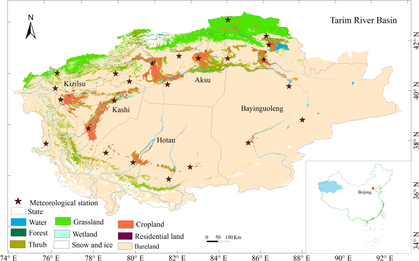
Fig. 1. The location and landuse map of the Tarim River Basin together with the meteorological stations.
Daily meteorological data were derived from the China Meteorological Administration (CMA, http://data.cma.cn/). This dataset was compiled through preliminary automated quality control and has been widely used in climate change related studies (Liu et al., Reference Liu2004; Zhai et al., Reference Zhai2005). Taking into account data availability and reliability, meteorological variables including the maximum, mean and minimum temperature (abbreviated hereafter as T max, T a and T min), wind speed (uz), sunshine duration (n), and maximum and minimum relative humidity (RH max and RH min) from 1960 to 2015 at 24 stations were used to calculate ET 0 and AWD (Table 1). Most stations are located in the oasis area of the Tarim River Basin (Fig. 1).
Table 1. Information of the meteorological stations in the Tarim River Basin and the average annual reference evapotranspiration (ET 0)

Calculation of reference evapotranspiration, crop water requirement and agricultural water demand
Figure 2 shows the calculation for the basin-scale AWD influenced by climate change and human activity. The Penman–Monteith approach, recommended by the UN Food and Agriculture Organization (FAO), was used to estimate ET 0 as it is widely recognized as being effective and efficient in calculating ET 0 (Allen et al., Reference Allen1998; Shen et al., Reference Shen2013). Reference evapotranspiration was defined and calculated based on the evapotranspiration of well-watered short grass of 0.12 m in height, resistance of 70 s/m and albedo of 0.23 (Allen et al., Reference Allen2005):
 $$ET_0 = \; \displaystyle{{0{\cdot}408\Delta (R_n - G) + \gamma \displaystyle{{900} \over {T_a + 273}}u_2(e_s - e_a)} \over {\Delta + \gamma (1 + 0{\cdot}34u_2)}}$$
where R n (MJ/(m2/day)) is the net daily radiation at the vegetation surface and the calculation of R n is dependent on sunshine hours (n) (measured at a meteoroogical station), as illustrated in McMahon et al. (Reference McMahon2013); G (MJ/(m2/day)) is the soil heat flux, which is generally assumed to be negligible for daily time-steps; u 2 (m/s) is the average daily wind speed at 2 m height observed at each meteorological station; e s (kPa) is saturation vapour pressure expressed as a function of measured T max and T min; e a (kPa) is mean daily actual vapour pressure calculated using measured T max, T min, RH max and RH min; Δ(kPa/°C) is the slope of the saturation vapour pressure curve, which is a function of observed mean daily temperature; and γ (kPa/°C) is the psychrometric constant. The detailed computation methods for these variables are given in McMahon et al. (Reference McMahon2013). The R-package ‘Evapotranspiration’ was applied to calculate ET 0 at each meteorological station on a daily basis (Guo et al., Reference Guo, Westra and Maier2016).

Fig. 2. Calculation procedure for the basin-scale agricultural water demand (AWD). The climate variables include maximum temperature (T max), minimum temperature (T min), wind speed (uz), sunshine hours (n), maximum relative humidity (RH max), minimum relative humidity (RH min). Human activity (planting structure factor) is represented by K cw.
The ETc of each crop at station j was calculated based on the crop coefficient approach (Eqn 2).
 $$ETc_{i,j} = K_{ci} \times ET_{0j}$$
where ETc i,j (mm) and K ci (-) are the crop water requirement and crop coefficient for the ith crop at station j. The controlling area of station j was defined by Thiessen polygon division (Fig. 3a). The K c value reflects the crop's relative water consumption capacity during different growing stages. It includes three parts: basal crop coefficient, the evaporative component of the bare soil fraction and the water stress coefficient (Calera et al., Reference Calera2017), and serves as an aggregation of the physical and physiological differences between a certain crop and the reference crop. In the current study, the five major crops covering the largest planting area, i.e. cotton, wheat, maize, rice and fruit trees, were considered. Other crops, including beet, potato, soybean, vegetable, oilseed rape and peanut, were not separately recorded due to their small planting areas (<0.16). Crop coefficients of cotton, wheat, maize, rice and fruit trees were derived from FAO recommendations (Allen et al., Reference Allen1998) and previous studies (Zhang et al., Reference Zhang, Zhang and Ma2010; Wang et al., Reference Wang2015). The intra-annual variations of K c values are shown in Fig. 3b.

Fig. 3. (a) Thiessen polygon division and the spatial variation of average annual reference evapotranspiration (ET 0) during 1960–2015. The red patches represent the farmland distribution with the light background indicating different states. (b) The intra-annual variations of crop coefficient during different growing stages (K c) of main crops in the Tarim River Basin. (c) Crop water requirement (ETc) of different crops based on ET 0 data at the Kashi meteorological station, which controls the largest irrigation area in the Tarim River Basin. (d) Agricultural water demand (AWD) for each state. (e) Variation of basin-averaged ET 0 and (f) Variation of basin-scale agricultural water demand (AWD) during 1960–2015.
AWD was a weighted average of ETc i,j:
 $$AWD{\rm \;} = \mathop \sum \limits_{i = 1}^N (ETc_{i,j} \times f_i){\rm \;} $$
where f i is the proportion of planting area for crop i and N is number of crop types (N = 5 in this case). Since the planting structure is only available for the five autonomous prefectures or states (i.e. Bayinguoleng, Aksu, Kizilsu, Kashi, Hotan), the area (proportion) of each crop f i at each Thiessen polygon was assumed to be the same as its closest state.
A quantitative indicator, K cw (i.e. weighted crop coefficient), was defined to represent quantitatively the impact of changings planting structures on regional water demand. It increases with the increase in area proportion of high water consuming crops:
 $$K_{cw{\rm \;}} = \mathop \sum \limits_{i = 1}^N (Kc_i \times f_i){\rm \;} $$
Traditional contribution analysis
The widely used contribution analysis (to differentiate it from the following numerical experiments, this method was referred to as ‘traditional analysis’) was applied to quantify the contribution of each meteorological factor and planting structure factor to AWD variation. The contribution index was defined by multiplying the response of AWD to a single factor by its relative change rate (McCuen, Reference McCuen1974; Li et al., Reference Li2017a):
 $${\rm S}_{Vi} = \mathop {\lim} \limits_{\Delta \to 0} \left( {\displaystyle{{\Delta AWD/AWD} \over {\Delta V_i/V_i}}} \right) = \displaystyle{{\delta AWD} \over {\delta V_i}}\displaystyle{{V_i} \over {AWD}}$$
 $${\rm Co}{\rm n}_{Vi,r} = {\rm S}_{Vi} \times \displaystyle{{L \times {Trend}_{Vi}} \over {\left \vert {\overline {Vi}} \right \vert}} \times 100$$
where S Vi is a unitless index meaing the response of AWD (mm) to factor Vi; ConVi,r (%) is the contribution of a driving factor V i to AWD variation; L is the number of years in one period. Trend Vi and  $\left\vert {\overline {V_i}} \right\vert$ are the annual trend and absolute mean value of V i; and ΔAWD and ΔV i are the variations of AWD and V i. If the contribution rate ConVi,r >0, then the factor variation promotes AWD increase, and vice versa. The higher the absolute value of ConVi,r, the greater contribution of factor V i.
Numerical experiment in contribution analysis
To disentangle different responses of AWD to forcing factors, several numerical experiments were designed to examine the AWD variation when the specific factors were free of any trends. To do that, a ‘Detrending’ approach was applied to remove the trends in these forcing factors.
Several numerical experiments were designed: (a) T max case (detrending all variables except T max); (b) T min case (detrending all variables except T min); (c) uz case (detrending all variables except uz); (d) n case (detrending all variables except n); (e) RH max case (detrending all variables except RH max); (f) RH min case (detrending all variables except RH min); (g) K cw case (detrending all the meteorological factors but K cw); (h) base case (detrending all forcing factors). The trends in AWD calculated from these experiments were compared with each other.
The simple and widely used ‘Detrending’ approach could eliminate the linear trend from the original meteorological variable (Zhang et al., Reference Zhang2016; Li et al., Reference Li2017b). Equation (7) illustrates how to remove the trends in variable T max and T min:
 $$T_{{\rm detrend},{\rm yr}} = T_{{\rm observed},{\rm yr}} - \beta ({\rm y}{\rm r}_{{\rm order}} - 1960)$$
where T detrend,yr (°C) and T observed,yr (°C) are the detrended and observed annual values, and β (°C/year) is the annual trend of T max or T min estimated based on least squares. yrorder denotes the year 1960, 1961,…, 2015.
For other meteorological factors and planting factor K cw, the Sen's slope estimator (Sen, Reference Sen1968) was used to determine the magnitude of change over time series. The Sen's slope method is a non-parametric method (Sen, Reference Sen1968) quantifying the linear median (50th percentile) concentration changes with time and is used to determine the magnitude of the trend line:
 $$Q_j = \displaystyle{{X_r - X_k} \over {r - k}},{\rm \; for\;} j = 1, \ldots, N;\,k \lt r \lt M{\rm \;} $$
where X r and X k are the data values at time r and time k, respectively. Normally, N = M(M−1)/2, where M is the length of data series. The Sen's slope β is then estimated as the median value of Q j. The trends in annual series were firstly removed by Eqn (9):
 $$F_{y-{\rm detrend},{\rm yr}} = F_{y-{\rm observed},{\rm yr}} - \beta ({\rm y}{\rm r}_{{\rm order}} - 1960)$$
where F y-detrend,yr is the detrended annual value of Vi in year yr and F y-observed,yr is original (i.e. observed) annual value in the same year. F y-detrend,yr and F y-observed,yr have the same units as the target variable V i. β (mm/yr for AWD, hour/year for n, etc) is the annual trend of Vi estimated using Sen's slope method. Then the annual ratio was applied to the daily timescale to generate a daily time series:
 $$F_{{\rm detrend,}d} = F_{{\rm observed},d} \times \displaystyle{{F_{y-{\rm detrend},{\rm yr}}} \over {F_{y-{\rm observed},{\rm yr}}}}$$
where F detrend,d and F observed,d are the detrended and observed daily values at day d in year yr. As with F y-detrend,yr and F y-observed,yr, F detrend,d and F observed,d have the same units as the target variable V i.
Finally, the detrended and observed variables were combined to generate AWD. To understand the influence level of each forcing factor on AWD, ConVi,e was applied to measure the contributions from different factors to AWD variation:
 $${\rm Co}{\rm n}_{Vi,e} = \displaystyle{{\delta AWD} \over {\delta V_i}}\displaystyle{{\delta V_i} \over t}$$
where ConVi,e (mm/yr) is the contribution of factor V i to AWD variation based on the numerical experiments.
Results
Spatial–temporal variations of reference evapotranspiration and agricultural water demand
Daily ET 0 at 24 stations were calculated and the distribution map of their mean annual values during 1960–2015 is displayed in Fig. 3a. The average ET 0 of these 24 stations was estimated to be 1163 mm, ranging from 796.6 to 1435.5 mm. Areas with large ET 0 were mainly distributed in low altitude regions, while low ET 0 values occurred mainly in high altitude regions (e.g. Bayanbulak51542, Baicheng51633, Turgat51701 and Tashi51804).
Figures 3c and 3d show the crop water requirements (ET c) of different crops at the Kashi station and regional AWD for the five states. Fruit trees had the highest ET c, approaching 1084.5 mm, followed by cotton (987.2 mm) and rice (778.9 mm), while ET c of wheat was the lowest (514.8 mm). Regionally, the AWD was estimated for each state. The highest AWD occurred in Bayinguoleng, and Kizilsu had the lowest AWD/m2. The time series of basin-averaged ET 0 and AWD during 1960–2015 are shown in Fig. 3. A turning point (year 1988) was detected based on Student's t method. The ET 0 demonstrated a decreasing trend during 1960–1988 (decreasing rate = 2.20 mm/yr) and then started to increase from 1989 (increasing rate = 4.62 mm/year). Agricultural water demand had a similar pattern to that of ET 0, with a turning point detected in 1988. It is worth noting that AWD has increased since 1989 at a very high rate of 9.47 mm/year. By 2010–2015, the AWD in the study region reached up to 826.1 mm/year. This represented a 16.4% increase from 683.7 mm/year during 1960–1988 to 795.9 mm/year since the beginning of the 21st century.
The variations of meteorological factors in the Tarim River Basin are shown in Fig. 4. T max and T min showed continuous increasing trends, with annual increases of 0.019 and 0.039 °C/year, respectively. uz and n show similar patterns of variation to ET 0 and AWD, which decreased over the period of 1960–1988 and then increased over 1989–2015. Meanwhile, RH max and RH min demonstrated substantial decreasing trends of 0.145 and 0.179%/year, respectively, since 1989. All the meteorological factors examined showed obvious increasing or decreasing trends, which favoured the increase of ET 0 and AWD during 1989–2015.

Fig. 4. Variations of the meteorological variables and planting structure factor (K cw) in the Tarim River Basin.
The proportions of crop acreages also changed since the 1980s, with an obvious decrease in wheat ratio (proportion of wheat area to agricultural acreage) and increasing ratios of cotton and fruit trees (proportions of cotton area and fruit tree area). As crop area data are not available before 1988, it was assumed that planting area during 1960–1988 was the same as that in 1988, which may not have been the case. The proportions of areas growing low-water-consuming crops (e.g. wheat, maize) exhibited a continuous decreasing trend, while high-water-consuming crops (e.g. cotton, fruit trees) have been increasing since 1988. The proportion of crop area given to fruit trees increased substantially from 8.15% during 1989–2000 to 29% by 2010 and then decreased slightly to 21.1% by 2015. The increases of crops with high water consumption led to increased K cw, especially for Bayinguoleng state (Fig. 4).
Quantifying the contributions of agricultural water demand variation
As the AWD showed an inverse trend during 1989–2015 compared with 1960–1988, the AWD variations during 1960–1988 and 1989–2015 were investigated. For each time period, the contribution of each forcing factor was quantified using both traditional contribution analysis and numerical experiments approach.
Table 2 summarizes the AWD trends in the Tarim River Basin and their attributions. A substantial decrease (−2.76 mm/year) was seen during 1960–1988 while obvious increase (9.47 mm/year) during 1989–2015. For the traditional contribution analysis, uz, RH max and n were detected to be the most important factors causing the decrease of AWD during 1960–1988 with the ConVi,r (i.e.  $S_{Vi} \times L \times {Trend}_{Vi}/\left\vert {\overline {Vi}} \right\vert \times 100$) being −7.82, −2.60 and −1.90%, respectively (Fig. 5). The contributions of uz computed by the traditional method ranged from −16.6 to −2.44%, with a mean value of −7.82% (Table 2).
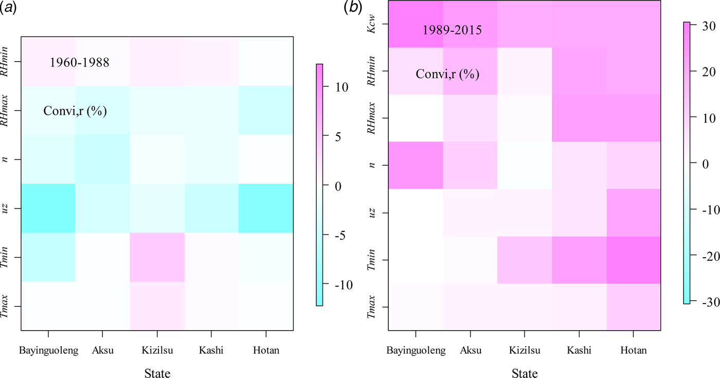
Fig. 5. State-scale contributions of the climate variables and human activities (measured by planting structure factor, K cw) to agricultural water demand (AWD) variations based on the traditional analysis (ConVi,r) for period 1960–1988 (a) and 1989–2015 (b).
Table 2. Contributions of meteorological factors and planting structure factor (represented by K cw) to agricultural water demand (AWD) variations based on traditional attribution analysis (ConVi,r) and numerical experiments (ConVi,e)

For numerical experiment, the trend of AWD (TrendAWD) of the base case (all meteorological factors and K cw were detrended) was 0.23 mm/year during 1960–1988 and 0.54 mm/year during 1989–2015, equivalent to relative changes of 0.9 and 2.0%, respectively. The results confirmed that the new detrended time series can be practically regarded as the base case to be compared against the following numerical experiments (Zhang et al., Reference Zhang2016). For period 1960–1988, T max and T min case resulted in average decrease rates for AWDs of 0.34 and 0.33 mm/year, respectively, comparable with that of the base case and indicating that T max and T min had negligible impact on AWD. The variation of uz alone was expected to lead to a dramatic decrease in AWD, with a decrease of 1.59 mm/year, which was recognized to be the dominant factor causing AWD decrease during 1960–1988. For the RH max and RH min case, RH max and RH min variations were suggested to cause decreases of 2.60 and 0.53 mm/year, respectively, in AWD. ConVi,erepresented the effect of factor V i to AWD variation base on the numerical experiments. ConTmax,e (i.e., (δAWD/δT max)(δT max/δt)) of the five states fell into the range of (–0.06, 0.68), with a mean value of 0.29 mm/year and an absolute mean value of 0.35 mm/year, indicating that T max has a negligible positive effect on AWD (Fig. 6). For the T min case, the  ${\rm Co}{\rm n}_{T_{{\rm min}},e}$ values fell into the range (–1.04–2.81) with a mean value of 0.73 mm/year and an absolute mean value of 1.15 mm/year, which meant that the contribution of T min to AWD was stronger than that of T max. The most important factor influencing AWD variation was also recognized to be uz, with the mean value being −7.01 mm/yr, followed by n and RH max. Meteorological factors, such as T max, T min and RH min had much smaller impacts on AWD compared with uz, n and RH max. The results were consistent with the findings based on the traditional analysis.
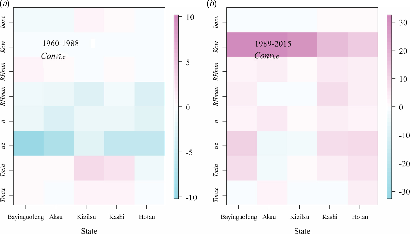
Fig. 6. State-scale contributions of climate variables and human activities (measured by planting structure factor, K cw) to agricultural water demand (AWD) variations based on a series of numerical experiments (ConVi,e) for period 1960–1988 (a) and 1989–2015 (b). Each row indicated one experiment. T max case (detrending all variables except for the maximum temperature); the T min (minimum temperature) case; the uz (wind speed) case; the n (sunshine hours) case; the RH max (maximum relative humidity) case; the RH min (minimum relative humidity) case; the K cw (planting structure factor, K cw, factor) case and the Base case (detrending all forcing factors).
Figure 7a demonstrates basin-scale contributions of meteorological factors and K cw to AWD variations. As K cw was considered to remain unchanged during 1960–1988, this means that the changes of observed AWD were caused merely by climate change. The impacts of climatic factors to AWD variation can be regarded as the differences between the observation (changing trend was −2.8 mm/year) and the base case (changing trend was −0.3 mm/year).

Fig. 7. Agricultural water demand (AWD) variations in the Tarim River Basin under different numerical experiments.
For the second period, 1989–2015, AWD increased dramatically with an average basin-scale increase rate of 9.47 mm/year. From the traditional contribution analysis, the variation of K cw contributed 24.76% of the AWD increment, followed in a descending order by T min, RH max, uz, RH min, n and T max (Table 2). For all states, K cw was the most prominent factor, with ConVi,r ranging from 18.70 mm/year to −12.5 mm/year, but especially for Bayinguoleng (Fig. 4).
For the numerical experiment, if all meteorological factors were detrended, the trend in K cw alone could result in an increase in AWD (Trend AWD) with a rate of 7.10 mm/yr. For T max, T min, uz, n, RH max and RH min, these meteorological factors had much weaker effects on AWD variation with Trend AWD values ranging from 0.62 to 1.45 mm/year (Table 2). The AWD trends caused by each meteorological factor were comparable to those of the base case (0.54 mm/year, detrending all the forcing factors) (Fig. 5).  ${\rm Co}{\rm n}_{T_{{\rm max}},e}$ (i.e. (δAWD/δT max)(δT max/δt) values) of the five states fell into the range of (–0.27,2.80), with the mean value being 0.95 mm/year and mean absolute value being 1.20 mm/year. ConVi,e caused by uz, T min and n were relatively higher, with the mean values being 4.76, 3.14 and 2.71 mm/year, respectively. The ConKcw,e was estimated to be the highest, indicating that the influence of K cw was the highest among all these forces. The increase in crop water requirement was caused mainly by the sharp increase in K cw since 1989. The effects of forcing factors on AWD variation were comparable to each other based on traditional contribution analysis. However, in the numerical experiment, the effect of K cw was identified as the most pronomient (dominant) factor resulting to the AWD increase.
Figure 7b shows different patterns of AWD variation during 1989–2015. The most significant increase was evaluated to be the observation, which was due to the positive impacts of both climate change and evolution of planting structure. The variation of K cw had a dominant effect on AWD, as the increment of AWD under the K cw case was 7.1 mm/year, much higher than that of the climate case (i.e. keeping K cw unchanged and keeping the original variations of meteorological factors) with increasing rate being 1.9 mm/year. The sharp increasing trend of observed AWD has turned to an apparent hiatus during 2008–2015, which was caused by the joint effects of both climate change (climatic variables did not show obvious trends) and human activity (K cw kept stable).
Discussion
Contribution of meteorological factors to agricultural water demand
Understanding AWD change is key to developing irrigation strategies, improving water use efficiency and understanding hydrological, climatic and ecosystem processes. With global warming, actual evapotranspiration (reflecting agricultural water use) over land increased from the early 1980s up to the late 1990s on a global scale (Wild et al., Reference Wild, Grieser and Schär2008; IPCC 2013).
Many previous studies investigated variation of reference evapotranspiration and its response to climate change (Rodríguez Díaz et al., Reference Rodríguez Díaz2007; Mo et al., Reference Mo2009; Shen et al., Reference Shen2013; Fan et al., Reference Fan2016). As argued by previous researches (Mo et al., Reference Mo2009; Li et al., Reference Li2017a), AWD variation was also related to meteorological factors other than the six factors used in the current study, which should also be taken into account to estimate AWD accurately.
In the current study, the variations of AWD was examined over the arid Tarim River Basin. Based on previous studies (Li et al., Reference Li2014; Guo et al., Reference Guo2015) and the current study, it was found that AWD decreased during 1960–1988 and then increased during 1989–2015. The contributions to the variation were analysed further. It was demonstrated that uz was the most prominent meteorological factor contributing to AWD variation during 1960–1988, which was consistent with those studies conducted in the arid north-west of China (Huo et al., Reference Huo2013; Li et al., Reference Li2014), the humid Haihe River Basin (Mo et al., Reference Mo2017), the arid Iran (Mosaedi et al., Reference Mosaedi2017), Spain (Rodríguez Díaz et al., Reference Rodríguez Díaz2007) and north-west Bangladesh (Acharjee et al., Reference Acharjee2017).
Crop types influence AWD dramatically (Zwart and Bastiaanssen, Reference Zwart and Bastiaanssen2004). If crop planting structure was not considered, the basin-scale AWD would still increase during 1989–2015, but with a much smaller slope (1.9 mm/year compared with the observed value of 9.47 mm/year). Evolution in crop structure could greatly promote the increase of AWD, which gives a strong signal that optimizing planting structure would be an effective water-saving strategy. As future climate change will affect the water balance of irrigated agriculture, farmers and irrigation managers could consider adapting to new scenarios by adjusting planting structure (Toureiro et al., Reference Toureiro2017).
However, an obvious disadvantage of the current study was that the climate change induced changes in growing season length and phenological stages of crops were not considered. For example, a combination of beneficial carbon dioxide (CO2) effects on plants, shorter growing periods and regional precipitation increases could lead to a decrease in global irrigation demand by ~17% (Konzmann et al., Reference Konzmann, Gerten and Heinke2013). It has been stated that when temperature increases by 1 °C, it can be expected that the growing season will decrease by 2 days and the water requirement will increase by 1.4 for spring wheat in the arid Heihe River Basin (Han et al., Reference Han2017). For the humid coasts of the Caspian Sea in Iran, crop water requirement of maize is expected to increase by 10.6–15.3% in the future, despite an obvious reduction in the length of the growing season (Karandish et al., Reference Karandish, Kalanaki and Saberali2017).
Potential water risk in the Tarim River Basin
In the Tarim River Basin, runoff is generated in the high mountains, recharged by glacier/snow melt water and precipitation. The oases could hardly survive without irrigation. Even though runoff has increased slightly due to more meltwater and slightly increased precipitation with current warming (Fang et al., Reference Fang2017), the increased area of irrigated land is consuming much more water than before. The water crisis is becoming more and more prominent, especially for some critical water-demanding periods, i.e. April, May and even June in some specific arable lands. This kind of seasonal water shortage reinforces water stress in the study region. As shown in the current study, the large proportion of high-water-consuming crops together with the unprecedented enlargement of crop growing area has resulted in a rapid increase in crop water demand. It has also already caused ecological degradation in the lower reaches of the Tarim River (Shen and Chen, Reference Shen and Chen2010; Shen et al., Reference Shen2013), such as the shrinkage of terminal lakes and the drying up of rivers (Chen et al., Reference Chen, Ye and Shen2011). Even though the Chinese government has put 10.7 billion RMB into implementing water-saving projects and guaranteeing water going downstream, serious problems (e.g. with improved canal water use efficiency, more and more land have been excessively, illegally cultivated) should also be recognized.
In addition, with further warming, glacier runoff will reach a peak in the coming years and the Shiyang River (Zhang et al., Reference Zhang, Gao and Zhang2015) will have less water in summer months (Fang et al., Reference Fang2017). The Tarim River Basin, the most important area for cotton and grain production, supports a population of 11 million people (Deng, Reference Deng2016). Therefore, it is urgent to implement water management such as regulation on water price and adjustment of crop planting structure, as well as water-saving technologies in this hyper-arid region, to cope with the ever more serious water crisis.
Conclusions
Agricultural water consumption, accounting for 95% of total water use in the Tarim River Basin, is the main factor affecting water resource allocation. Based on the Penman–Monteith equation and crop coefficient approach, crop water requirement since 1960 was estimated and the contributions of meteorological factors and planting structure to AWD variation were quantified. The following conclusions can be drawn:
(1) AWD experienced a decreasing trend during 1960–1988 with a rate of −2.76 mm/year; but then increased from 1989 at a very high rate of 9.47 mm/year.
(2) Wind speed and sunshine hours decreased over the period 1960–1988 and then increased from 1989–2015. The proportions of planting area of high water-consuming crops (e.g. cotton, fruit trees) have increased.
(3) The traditional contribution analysis method and the numerical experiment approach generated consistent results. For 1960–1988, the most significant factor inducing AWD variation was wind speed (uz), followed by RH max and sunshine duration (n); other meteorological factors were not as important as these three. For 1989–2015, the dominant factor affecting AWD was K cw (representing the weighted K c values caused by the evolution of planting structure). The application of two different contribution analysis methods could provide robust results and these conclusions will shed light on detecting effective approaches for future water-saving strategies.
Financial support
This work was supported by the CAS ‘Light of West China’ Program (grant no. 2016-QNXZ-B-12), the National Natural Science Foundation of China (grant no. 41701043) and the Strategic Priority Research Program of Chinese Academy of Sciences (grant no. XDA20100300).
Conflicts of interest
None.
Ethical standards
Not applicable.


