


Introduction
In numerous applications, the operating environment of antennas modifies their radiating properties. This is the case, for example, for on-body communicating sensors, embedded antennas interacting with their physical support or keyless access antennas coupled to the ground in the automotive domain, etc. Suitable techniques have to be developed to obtain a reliable knowledge of the far-field characteristics taking the surroundings into account. For example, in our case of study, we are interested in UHF scaled-down models of HF radar antennas, as the dimensions of HF antennas are too large for indoor measurements. The near-field to far-field transformation (NF/FF transformation) is one of the techniques used to characterize antennas. It takes the place of direct far-field measurements when these latter are not practicable. The principle consists in deriving the far-field radiated by an antenna from near-field information.The classical NF/FF transformation relies on wave mode expansions [Reference Yaghjian1,Reference Schmidt, Leibfritz and Eibert2]. But for almost 25 years, another approach, based on the equivalence principle, has also been developed [Reference Sarkar and Taagho3]. This method requires the generation of equivalent sources (electric and/or magnetic dipoles, electric currents) to derive the radiation pattern of the antenna. In the literature, whatever the chosen procedure, most cases are about free-space configurations [Reference Alvarez, Las-Heras and Pino4]. In only few ones, an image theory, involving Fresnel reflection coefficients, is applied to estimate the image equivalent currents due to the ground [Reference Sugimoro and Arai5–Reference Schmidt and Eibert7]. But this approach does not allow taking into account some specific wave modes as the surface or leaky waves, for example. For this reason, a specific NF/FF transformation has been developed. It is based on data extracted from a measurement, in the near-field zone, of the electric field radiated by an antenna, located in the vicinity of an actual ground, which properties are assumed to be known. We choose, for convenience, to perform the measurement at UHF frequencies with a scaled-down model of HF antennas. The objective is to prove, at higher frequency (for which the experimental set-up is easier to carry out), the validity of our approach to estimate the far-field of antennas usually used at lower frequency (HF band) known to support specific wave modes like surface wave. This paper is organized as follows. In section “Near-field to far-field transformation”, a description of the method is given. In section “Experimental set-up”, the experimental set-up, used to validate the approach, is described. In section “Experimental results”, theoretical and experimental results, obtained with UHF antennas, are compared. Finally, a conclusion and perspectives are drawn.
Near-field to far-field transformation
The transformation method is based on source identification, assuming that the antenna under test (AUT) can be replaced by a set of equivalent uncoupled elementary dipoles radiating the same far-field as the AUT. The dipole radiation functions are based on the analytic formulations developed by Norton [Reference Norton8] and extended by Bannister [Reference Bannister9] to the very near-field zone. These formulations of the electromagnetic field radiated by each dipole comprise the sky wave, which is the sum of the direct and reflected waves, as well as the surface wave contribution. Such an approach has already been introduced in [Reference Payet, Darces, Montmagnon, Hélier and Jangal10] and necessitates the sampling of both the electric and magnetic near-fields. Such a process requiring the measurement of the three components of two physical quantities could be very time consuming. Otherwise, magnetic probe are not very widespread and are also expensive. To overcome those difficulties, a simple solution is to estimate the magnetic field from the electric field by a plane wave approximation. This approximation has already been justified in [Reference Djoma, Darces and Hélier11].
Let us consider an AUT located at the plane horizontal interface between the air and the actual ground as shown in Fig. 1(a). The components of the electromagnetic field are measured in the near-field zone on a surface S M surrounding the AUT. For convenience, S M is a cylindrical surface, of radius r SM and height h SM, centered on the AUT (Fig. 1(b)). The number of measurement points on surface S M is N M. Let us consider now a second surface S D, included inside the volume delimited by surface S M. Also, for convenience, surface S D is supposed to be a cylinder of radius r SD and height h SD, centered on the AUT (Fig. 1(b)).
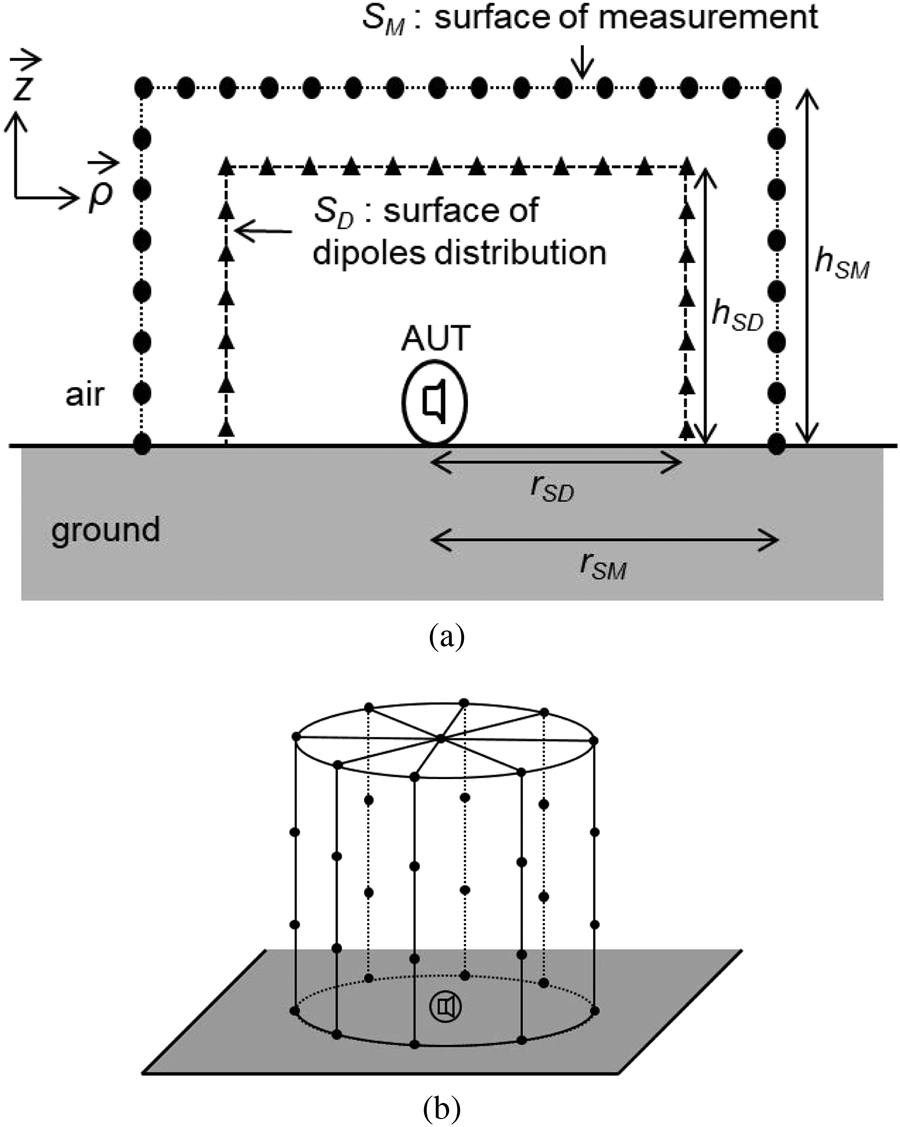
Fig. 1. Geometry associated to the method: (a) general view (b) cylindrical surface enclosing the AUT.
The number of sampling points on surface S D is N D. At each point, three elementary virtual electric dipoles are arranged in order to form an orthogonal basis aligned with the local cylindrical basis vectors. The method states that, at each point of the surface S M, the electromagnetic field is equal to the sum of all the contributions coming from each of the 3N D dipoles distributed over the surface S D. This leads to the following matrix equation:
 $$ \left[\matrix{ {{D_E}} \cr {{D_H}} }\right]\left[ P_{S_D}\right] = \left[\matrix{ E_{{S_M}} \cr H_{{S_M}} }\right] $$
where  $E_{S_M}$ and
  $H_{S_M}$ denote the electric and magnetic vector fields of size 3N M, measured at each point on the surface S M. As mentioned previously, the magnetic field
  $H_{S_M}$ is actually derived from the measurement of the electric field
  $E_{S_M}$considering a plane wave approximation. D E and D M are the electric and magnetic radiation matrices, each of size 3N M × 3N D, of the 3N D electric (horizontal and vertical) dipoles located at each point of the surface S D. P SD is the unknown vector, of size 3N D, gathering the electric moments of the previous dipoles. Equation (1) can be solved by inversion of the radiation matrix
  $\left [\matrix{{c} D_E \cr D_H }\right]$ in order to compute the vector P SD.
At the first step of the transformation, all the elementary dipoles are taken into account as possible contributors to the radiation. To optimize that transformation, it is advisable to select and keep only the dipoles which have a significant contribution to the total field. To achieve that goal, the inversion of the radiation matrix is carried out by applying a singular value decomposition (SVD) associated with a threshold power criterion. The criterion is based on the total power radiated by the AUT, in the near-field zone. It is calculated from the electric field measured on surface S M and the magnetic field estimated from the electric field. This power criterion is compared to the sum of the total power radiated by the current set of elementary electric dipoles through the surface S M. The singular values of the radiation matrix (and the associated dipoles) are removed one by one from the smallest one until the corresponding calculated power matches the power criterion. Once the vector P SD is obtained, the electric far-field can be easily computed.
Experimental set-up
An experimental set-up has been designed in order to characterize antennas, in operating environment, in the UHF band [Reference Bourey, Darces and Hélier12]. The main element of the set-up is the probe system [13] and is shown in Fig. 2. This probe measures the component of the electric field parallel to the axis of its head namely E m in Fig. 2(b). This axis can be modified, thanks to a mechanical device, in order to successively acquire the three orthogonal components of the electric field. The probe head is linked to its base unit by means of an optical fiber cable. The reduced size of the probe head ensures negligible couplings with the AUT and the optical link avoids electromagnetic disturbances. A two-port vector network analyzer is used, as shown in Fig. 3. Its port 1 feeds the AUT and its port 2 is connected to the RF output of the base unit. The corresponding complex transmission coefficient S 21 is firstly corrected in phase in order to compensate for the length of the optical fiber cable. It leads to the corrected transmission coefficient S 21c given by:
 $$ {S_{21c}} = {S_{21}}.{e^{{\rm{i}} { 2\pi f\delta}}} $$
where f is the carrier frequency and δ is the duration of the propagation in the optical fiber.

Fig. 2. Electric field probe: (a) base unit of the probe system, (b) probe head over a brass plate.

Fig. 3. Electric field measurement set-up.
The magnitude of the complex electric field E m is related to the voltage V m at port 2 by means of the antenna factor of the probe AF, depending of the frequency:
 $$ \left\vert {E_m}\right\vert ={AF}.\left\vert {V_m}\right\vert . $$
The power of the signal received at port 2 is given by:
 $$ {\left\vert {S_{21}}\right\vert }^2.{P_{in}}={{\left\vert {V_m}\right\vert }^2 \over Z_2}, $$
where P in is the power supplied to the AUT and Z 2 is the input impedance of port 2. Finally, the complex electric field E m is obtained from the following equation:
 $$ {E_m} = {AF}.\sqrt {{{\left\vert {{S_{21c}}} \right\vert }^2}{P_{in}}{Z_2}}. {e^{{\rm{i}}\,\arg S_{21c}}}. $$
An image of the global set-up is depicted in Fig. 4. To acquire the value of the electric field on the whole surface S M, three motorized linear guides allow the displacement of the probe head in the working volume. The AUT is located on a horizontal plane interface which dielectric properties can be changed (perfect electric conductor, lossy ground, metasurface, etc.). A rotating axis adjusts the azimuthal position of the AUT. The working volume is surrounded by electromagnetic absorbers. For each displacement of the head probe, the transmission coefficient and position data are stored. The standard antialiasing criterion defines the steps Δρ, Δϕ, and Δz between two adjacent points and can be expressed as:
 $$ \Delta \rho \le {\lambda \over 2}\quad \Delta \phi \le {\lambda \over {2{r_{SM}}}} \quad \Delta z \le {\lambda \over 2}. $$
where λ is the free-space wavelength.

Fig. 4. Global set-up.
Experimental results
In order to validate our approach, we have compared our results with those obtained through a full-wave simulation performed with the commercial software FEKO. On the one hand, the measurement of the near electric field are compared with near-field simulations made with FEKO. On the other hand, the far electric field derived with the NF/FF transformation are compared with the direct far-field computed with FEKO. Two types of antennas have been studied. In the first case, the AUT is an array of three monopole antennas located over a large sheet of brass. In the second case, the AUT is a wideband biconical antenna located over a sandy land. In both cases, the operating frequency is 1 GHz.
Three quarter wavelength monopole antennas
The AUT is an array of three monopole antennas as shown in Fig. 5, each antenna separated from the nearby one by a distance λ/2 and located over a large sheet of brass. The measurement surface S M depicted in Fig. 1 is such as r SM = 1.5λ, h SM = 1.5λ, and the number of measurement points is N M = 681. The surface of dipoles distribution S D is such as r SD = λ, h SD = λ, and the number of dipole positions is N D = 482. After the SVD, the number of singular values required to model the AUT is equal to 212 in that case. From a computational point of view, the derivation of the dipole moments required 17 min with a 3.5 GHz Intel Xeon W-2135 Hexa-Core processor and 64 Go memory.

Fig. 5. An array of three quarter wavelength monopole antennas.
We have made a comparison between experimental results and those obtained from a FEKO simulation assuming that the three antennas are fed with the same current. Figure 6 shows the magnitude of the two cylindrical components  $E_\rho $ and E z of the electric field at distance r SM along a vertical line (parallel to the z axis) for different values of the azimuthal angle ϕ. The results are in good agreement, particularly for the vertical component, which is the highest of the two ones.

Fig. 6. Comparison between electric near-field measurements and simulations with FEKO for different azimuthal angles ϕ at 1 GHz and at distance r SM: (a) radial component E ρ, (b) vertical component E z.
Based on those near-field measurements, we have computed the far-field resulting from the NF/FF transformation and compared it with the direct far-field simulated by FEKO at the same distance. Figure 7 shows the magnitude of the spherical θ-component of the electric field, as a function of angle θ, at distance R = 10λ for various angles ϕ. Whatever the azimuthal ϕ and zenith θ angles, the results are in very good agreement. This first example illustrates the fact that the NF/FF transformation is suitable and reliable for the determination of the far-field radiation of directional antennas. The corresponding time consuming for the calculation of the far-field with the NF/FF transformation is about 2.5 min.

Fig. 7. Comparison between electric far-field calculated with the NF/FF transformation and electric far-field computed with FEKO for different azimuthal angles ϕ at 1 GHz and at distance R = 10λ = 3 m.
Wideband biconical antenna
In that second case, the AUT is a wideband biconical antenna as shown in Fig. 8. This antenna is a scaled-down model of a classical HF biconical antenna used for the HF over-the-horizon radar. The antenna is located over a representative ground chosen as a handmade sandy land with the following characteristics obtained by means of the electromagnetic similitude principle: relative permittivity εrr = 12.2 and conductivity σ = 0.25 S/m. This soil is a mixing of common sand, water, and copper sulfate and has been characterized following the procedure described in [Reference Belhadj-Tahar, Meyer and Fourier-Lamer14].

Fig. 8. Biconical antenna: (a) 1/100 scale model of HF biconical antenna. (b) Model of the biconical antenna over a sandy land with a bounded metallic ground plane required for a good matching.
As in the previous case, we have made a comparison between near-field FEKO simulations and measurements. The measurement surface S M is such as r SM = 1.4λ, h SM = 1.5λ, and the number of measurement points is N M = 2017. The cylindrical surface of dipole distribution S D is such as r SD = λ, h SD = λ, and the number of dipole positions is N D = 482. After the SVD, the number of singular values required to model the AUT is here equal to 335. From a computational point of view, the derivation of the dipole moments required 35 min with the same 3.5 GHz Intel Xeon W-2135 Hexa-Core processor and 64 Go memory. Due to the omnidirectional property of such an antenna in azimuth, the electric fields are plotted in only one azimuthal direction.
Figure 9 shows the magnitude of the two cylindrical components  $E_\rho $ and E z of the electric field at distance r SM along a vertical line (parallel to the z axis). Experimental and simulation results are in good agreement, particularly for the component with the highest magnitude, E z.

Fig. 9. Comparison between electric near-field measurements and simulations with FEKO at 1 GHz and at distance r SM: (a) radial component E ρ, (b) vertical component E z.
Again, we have compared the results of the NF/FF transformation with the direct far-field computed by FEKO at the same distance, as the sky wave and the surface wave depend differently on distance. Figure 10 shows the magnitude of the spherical θ-component of the electric field, as a function of angle θ, at two distances R = 3λ and R = 10λ. The results are in good agreement anew. The NF/FF transformation allows the calculation of the spatial distribution of the electric far-field radiated by an antenna in its operating environment. The decrease of the surface wave (visible at angle θ = 90°) with the observation distance can be predicted, in particular. The corresponding time consuming for the calculation of the far-field with the NF/FF transformation is also about 2.5 min.

Fig. 10. Comparison between electric far-field calculated with NF/FF transformation and electric far-field computed with FEKO at 1 GHz and distance: (a) R = 3λ, (b) R = 10λ.
Conclusion
A near-field to far-field transformation suitable to predict the radiation of antennas in their operating environment has been developed, described, and tested. The theoretical content of the transformation has been detailed. That transformation allows to replace the AUT by an equivalent set of virtual dipole sources. A specific UHF experimental set-up has been designed to assess the method. Firstly, the near-field characterization on an array of three monopoles over a metallic ground plane has given rise to the reliable calculation of the far-field radiation in various azimuthal directions. The case of directional antennas can hence be handled by the proposed approach. Secondly, it has been shown that the far-field radiated by a biconical antenna over a sandy ground can be successfully predicted. As a consequence, the case of an antenna in a Sommerfeld half-space problem can also be processed. The transformation as well as the experimental protocol have been validated in the UHF band.
Now, some perspectives are emerging. They take place in the context of the characterization of the antennas employed in over-the-horizon radar systems, operating at lower frequencies, as mentioned in the Introduction. The first idea is about the near-field characterization of full-scale HF antennas in actual operating conditions by means of a drone, as the direct measurement of the far-field of these antennas is very expensive (a helicopter may be required) or unworkable. The second one aims at the estimation of the electric field radiated by a metamaterial structure when specific propagation modes, like surface wave mode, are fostered. Full-scale HF and scaled-down UHF devices will be considered.
Acknowledgments
The authors thank warmly the French MoD (DGA) for its scientific and financial support.
 N. Bourey was born in Versailles, France, in November 1986. He received the M.S. degree in ElectronicsEngineering in 2011 from Pierre et Marie Curie University, France. From 2011 to 2014, he was a Ph.D student at Pierre et Marie Curie University, France. In 2014, he received his Ph.D in Engineering Sciences with Onera – The French Aerospace Lab, Palaiseau, France. In 2016, he was a post-doctoral fellowship at Royal Military College in Kingston, Canada. From 2017 up to now, he is a post-doctoral fellowship at Sorbonne UniversIty in Paris, France. His current research activities include electromagnetic wave propagation and metamaterials.
 M. Darces received her M.S. degree in Electrical Engineering in 1994 and her Ph.D. degree in 1997 from Pierre et Marie Curie University, Paris, France. From 1998 to 2001, she was an assistant professor at Claude Bernard University, Lyon, France. Since 2002, she is an assistant professor at the Laboratoire d'Électronique et Électromagnétisme at Sorbonne University, Paris, France. Her current research concerns electromagnetic wave propagation, HF radar applications, and EMC.
 Y. Chatelon was born in Conflans Sainte Honorine in 1956. After 3 years of medical studies, he decided to learn electronic basis to get a job in the medical field companies during 10 years. After a university-level degree program in Mechanics and Productics, he followed by studies in Aerodynamics, he joined the CNAM (Conservatoire National des Arts et Métiers) in Paris, France, asa technician at the Aerodynamics dpt. He had the opportunity to join Pierre et Marie Curie University in 2010 asa manager of the PIC (Platform for Instrumentation and Characterization) of L2E (Laboratoire d'Électronique et Électromagnétisme) where he is in charge of all experimental sides, whether electronics or mechanical projects.
 M. Hélier was born in Paris in 1958. He received the “diplôme d'ingénieur” degree from the École Supérieure d'Électricité (France) in 1981 and the Ph.D. degree from Paris-Sud University in 1983. As an assistant professor, he was with the ESIEE (Ivory Cost) from 1983 to 1984 and with the École Supérieure d'Électricité from 1985 to 2001. Since 2001, he is a full professor at Pierre and Marie Curie University, known since 2018 as Sorbonne University. He was the head of the Laboratoire d'Électronique et Électromagnétisme (L2E) from its setting up in 2008 to the end of 2011. From 2012 to 2017, he was the director of the Education and Career Guidance Directorate of Pierre and Marie Curie University. Since 2018, he serves as an advisor to the Vice-President of Sorbonne University for Research, Innovation, and Open Science. His current research area focuses on EMC and HF antennas.


