2.1. Facility

All experiments are carried out in the Air Force Research Laboratory (AFRL) Mach-6 Ludwieg tube, an impulse facility capable of producing two steady-flow test periods, each of approximately 100 ms, per experiment (Kimmel et al. Reference Kimmel, Borg, Jewell, Lam, Bowersox, Srinivasan, Fuchs and Mooney2017). For each experiment presented in the current study, the second steady-flow period is used to acquire measurements. In the current investigation, free-stream unit Reynolds numbers are set between $4.90\times 10^{6}$ and $22.71\times 10^{6}\ {\rm m}^{-1}$ for individual runs by adjusting the reservoir pressure between 689 kPa and 3.48 MPa. Flow is initiated using a fast-acting valve, and air is used as the test gas. The nozzle throat is 9.42 cm in diameter with an exit diameter of 76.2 cm that terminates in a test chamber approximately 1.27 m in diameter. Optical access is provided by 30.5 cm diameter windows on both sides of the test section. Additional free-stream conditions for each experiment can be found in table 1, and additional information on the facility can be found in Kimmel et al. (Reference Kimmel, Borg, Jewell, Lam, Bowersox, Srinivasan, Fuchs and Mooney2017).

Table 1. Tunnel free-stream conditions.

2.2. Model

The test article is a $7^{\circ }$ half-angle, slender cone with an interchangeable nose section. With the sharp nose installed, the cone length is 414 mm. Five nose tips of different radii ranging from nominally sharp to 5.08 mm are tested and, for consistency, the surface coordinate $s$ used hereinafter refers to the streamwise distance measured from the tip of the sharp-nose configuration. For all experiments, the model is installed at zero incidence (${\pm }0.5^{\circ }$) to the free stream. The cone is equipped with eight PCB Piezotronics model 132A and 132B piezoelectric pressure transducers for measuring high-frequency (${>}$11 kHz) pressure fluctuations. Six of the PCB sensors lie along a single streamwise ray as shown in figure 1. The two additional PCB sensors are placed adjacent to the sensor located at $s=316\ {\rm mm}$ and are offset in the circumferential direction by 5.715 mm on either side relative to this plane. The three-sensor-wide array allows for measurements of the spanwise distribution of pressure disturbances. The signals from the PCB sensors are recorded at 5 megahertz. Prior to the start of all experiments, the model is at room temperature, resulting in a wall-to-stagnation temperature ratio of approximately 0.6.

Figure 1. Schematic showing instrumentation layout on cone model with sharp-nose configuration. The red dots indicate the PCB sensor locations.

2.3. Schlieren visualizations

A conventional Z-type (non-focusing) schlieren set-up is utilized to visualize the flow density gradients. Illumination is provided by a Cavilux HF pulsed-diode laser emitting pulses of 30–40 ns duration at 810 nm, released from a 1.5 mm diameter fibre-optic cable. Two 31.8-cm diameter, 1.91-m focal length mirrors are used to collimate the light to pass through the test section and refocus it on the other side. A knife-edge cutoff is used to visualize the density gradients normal to the cone surface, and a Phantom v2512 high-speed camera mounted parallel to the cone surface records the images. For all experiments, the image resolution in the horizontal direction is 1280 pixels, while the number of pixels in the vertical direction is chosen based on the desired camera frame rate and pixel scale. In general, the frame rate is set to be at least one half of the second-mode fundamental frequency predicted by the linear PSE (LPSE), and the number of pixels across the boundary-layer thickness ranges from a minimum of approximately 8 to a maximum of 30. Camera parameters for each experiment are shown in table 2, and an example schlieren image from experiment S1 is shown in figure 2. The slow spatial evolution of the second-mode waves relative to the image acquisition rate allows for the application of the time-signal-reconstruction technique developed in Kennedy et al. (Reference Kennedy, Laurence, Smith and Marineau2018). For the present experiments, the reconstruction technique is only applied for the cases where the boundary-layer behaviour is dominated by second-mode waves, corresponding to nose-tip radii less than or equal to 1.524 mm. Temporal signals are reconstructed using 3000 images per experiment at 100 streamwise locations evenly spaced across the visualization region.

Table 2. Cone model and camera parameters used for each experiment. The entropy-layer swallowing distance, $X_{SW}$, and edge Mach number, $M_{e}$, are computed as described in § 2.4; the latter is calculated at the centre of the visualization region.

Figure 2. Enhanced schlieren visualization generated by subtracting a mean flow-on image from the image of interest for the sharp nose-tip-radius configuration experiment S1.

Calibration of the schlieren system following Hargather & Settles (Reference Hargather and Settles2012) is performed to enable quantitative measurements. Calibration is required due to the nonlinear schlieren response of the light rays generated by the circular light source. Prior to the start of each experiment, a circular plano-convex lens with a diameter of 25.4 mm and a focal length of 10 m is placed within the schlieren field of view. The incoming collimated light rays are deflected to a degree depending on where they pass through the calibration lens; this in turn causes a pixel-intensity gradient to form across the visualized lens face. The pixel intensity at any point on the lens face can then be correlated with the known density gradient generated by the calibration lens. For more details associated with the calibration procedure, see Kennedy (Reference Kennedy2019).

2.4. Computational method

Computational analysis is performed using the STABL software suite described by Johnson, Seipp & Candler (Reference Johnson, Seipp and Candler1998), Johnson (Reference Johnson2000), Johnson & Candler (Reference Johnson and Candler2005), and implemented in Jewell (Reference Jewell2014) and Wagnild et al. (Reference Wagnild, Candler, Leyva, Jewell and Hornung2010), as well as the instability analysis solver developed by Paredes (Reference Paredes2014) and Paredes et al. (Reference Paredes, Hanifi, Theofilis and Henningson2015). First, the mean flow over the cone is computed by the reacting, axisymmetric Navier–Stokes equations with a structured grid, using a version of the NASA data parallel-line relaxation (DPLR) code (Wright, Candler & Bose Reference Wright, Candler and Bose1998). This flow solver is based on the finite-volume formulation. The use of an excluded volume equation of state is not necessary for the boundary-layer solver because the static pressure over the cone is sufficiently low (typically, 1–5 kPa) that the gas can be treated as ideal. The mean flow is computed on a single-block, structured grid with dimensions of 361 cells by 359 cells in the streamwise and wall-normal directions, respectively. The inflow gas composition in each case is air with 0.233 O$_2$ and 0.767 N$_2$ mass fractions, and the impact of chemical reactions is negligible as the local maximum temperature does not exceed 550 K for any case.

Grids for each of the five bluntness configurations were generated using STABL's built-in grid generator, and mean-flow solutions were examined to ensure that at least 100 points were placed in the boundary layer for each stagnation pressure. The boundary-layer profiles and edge properties are extracted from the mean-flow solutions during post-processing. The wall-normal span of the grid increases down the length of the cone, from 0.25 mm at the tip to 50 mm at the base, allowing for the shock to be fully contained within the grid for all cases tested. The grid is clustered at the wall as well as at the nose in order to capture the gradients in these locations. The $\Delta y^+$ value for the grid, extracted from the DPLR solution for each case, is everywhere less than 1, where $\Delta y^+$ is a measure of local grid quality at the wall in the wall-normal direction. Linear PSE stability analyses are performed using the PSE-Chem solver, which is also part of the STABL software suite. The PSE-Chem (Johnson & Candler Reference Johnson and Candler2005) software solves the reacting, two-dimensional, axisymmetric, linear PSEs to predict the amplification of disturbances as they interact with the boundary layer. As the temperatures remain sufficiently low, chemistry and molecular vibration effects are omitted. Following Marineau, Moraru & Daniel (Reference Marineau, Moraru and Daniel2017), a linear function is used to fit the LPSE maximum $N$ factor versus stability Reynolds number ($R$) results, and a function of the form $f=g/R^{h}$, where $g$ and $h$ are constants, is used to fit the LPSE results of most-amplified second-mode frequency versus stability Reynolds number for comparison to the experimental measurements. Estimates of the entropy-layer swallowing length as defined by Rotta (Reference Rotta1966) are computed using a procedure based on Stetson (Reference Stetson1983) to provide an empirically based estimate of the extent of the entropy-layer influence.

The linear non-modal and nonlinear PSE (NPSE) stability analyses are performed following the methodology described by Paredes et al. (Reference Paredes, Choudhari, Li, Jewell and Kimmel2019b) and Paredes, Choudhari & Li (Reference Paredes, Choudhari and Li2020). The methodology used for the analysis of non-modal disturbance amplification over the blunt cone configuration is performed using the harmonic linearized Navier–Stokes equations (HLNSE) as explained by Paredes et al. (Reference Paredes, Choudhari, Li, Jewell, Kimmel, Marineau and Grossir2019c). A variational formulation is used to determine the optimal inflow disturbance that leads to maximum energy gain at a specified downstream position. The HLNSE are discretized with sixth-order finite-difference schemes along the streamwise and wall-normal coordinates. The discretized NPSE are integrated along the streamwise coordinate by using second-order backward differentiation. Sixth-order finite-difference schemes are used for discretization of the NPSE along the wall-normal coordinate. The maximum number of Fourier modes is set to 12.

3.1. Time-averaged results

We begin our analysis by considering the three experiments performed with the sharp-nose model configuration, for which the second-mode instability is expected to be the dominant transition mechanism (S1–S3). The mean wavepacket propagation speeds, $u_{prop}$, are determined using the image correlation methodology described in Laurence et al. (Reference Laurence, Wagner and Hannemann2014). The images are first processed by a feature detection algorithm to identify the presence and, if applicable, location of a wavepacket. The images are then bandpass filtered around the second-mode fundamental wavelength and a cross-correlation is applied to image pairs throughout the sequence. The mean wavepacket propagation speeds and 95 % error bounds calculated for each condition using approximately 8000 wavepackets per experiment are $787\pm 28.2\ {\rm ms}^{-1}$, $778\pm 53.4\ {\rm ms}^{-1}$ and $804\pm 36.4\ {\rm ms}^{-1}$ for experiments S1, S2 and S3, respectively. Using the Taylor–MacColl solution to compute the cone surface conditions and assuming that these correspond to the boundary-layer edge conditions, we obtain $u_{prop}/u_{e}=0.94\text {--}0.97$, roughly in line with the previous measurements of Kimmel & Kendall (Reference Kimmel and Kendall1991), Laurence et al. (Reference Laurence, Wagner and Hannemann2016) and Kennedy et al. (Reference Kennedy, Laurence, Smith and Marineau2018). Using the reconstructed time signals described in § 2.3, spectra are computed using Welch's method and used to identify the most-amplified second-mode frequencies and amplitudes for each downstream location and experimental condition. Example spectra computed from time signals reconstructed at three streamwise locations for experiment S3 are observed in figure 3. The amplitude of the content at the fundamental second-mode frequency (approximately 240–290 kHz) is observed to increase with increasing downstream location, while the second-mode frequency decreases due to the increasing boundary-layer thickness. Following Stetson (Reference Stetson1983), the dimensionless most-amplified second-mode frequency is defined as

(3.1)\begin{equation} F = \frac{2{\rm \pi} f_{{max}}}{u_{\infty}Re/m}, \end{equation}

and the stability Reynolds number is defined as

(3.2)\begin{equation} R = \sqrt{Re_{s}}, \end{equation}

where $u_{\infty }$ is the free-stream velocity, $Re$ is the Reynolds number based on the free-stream conditions, $f_{{max}}$ is the most-amplified second-mode frequency and $s$ is the cone surface coordinate.

Figure 3. Spectra computed using reconstructed time signals from schlieren visualizations from experiment S3 at three different streamwise locations.

In figure 4 we present dimensionless most-amplified second-mode frequencies. In the left plot, measurements are shown for each unit-Reynolds-number condition along with LPSE results, and in the right plot, measurements are shown for experiment S3 along with both LPSE and NPSE results. The NPSE results are computed using an initial disturbance with a finite streamwise velocity at a frequency equal to the measured most-amplified disturbance frequency at $R=1585$ in experiment S3. Computations are presented for two different streamwise velocity initial amplitudes, where $\tilde {u}_{0}$ refers to the root-mean-square of the streamwise velocity disturbance normalized by the free-stream velocity. In the left plot of figure 4, good agreement is observed between the frequencies measured using the schlieren visualizations and PCB sensors. Across the measurement region, the LPSE overpredict the frequencies by approximately 5 %. In figure 4(b) it is observed that the addition of nonlinear effects in the NPSE computation leads to better agreement between the measurements and computations, as increasing the initial disturbance amplitude decreases the most-amplified second-mode frequencies. It is also noted that slight misalignment of the cone from zero incidence, but within the model installation accuracy of ${\pm }0.5^{\circ }$, may also contribute to a change in the experimentally observed second-mode frequencies and cause disagreement between the measured and computed results (see, for example, Hofferth, Humble & Floryan Reference Hofferth, Humble and Floryan2013).

Figure 4. Most-amplified second-mode frequencies. (a) Experimental results for S1, S2, S3 shown with LPSE results. (b) Experimental results for S3 shown with LPSE results and NPSE results computed for disturbances with different streamwise velocity initial amplitudes. The data correspond to: (-$\bigcirc$-), S1; (-$\Diamond$-), S2; (-$\Box$-), S3; (–), LPSE; (- $\cdot$), NPSE, $\tilde {u}_{0}=5\times 10^{-4}$; (- -), NPSE, $\tilde {u}_{0}=1\times 10^{-3}$. Filled symbols are schlieren measurements, while open symbols are PCB measurements.

Maximum $N$ factors are computed here as

(3.3)\begin{equation} N(f_{{max}},s_{i}) = \tfrac{1}{2}\ln(\textrm{PSD}(f_{{max}},s_{i}))+c, \end{equation}

where PSD($f_{max},s_{i}$) is defined as the peak power of the most-amplified second-mode frequency at streamwise location $s_{i}$, and $c$ is the vertical intercept identified by vertically shifting the schlieren measurements to match the LPSE curve. This vertical shift is required as the most upstream measurement location of the schlieren visualizations is downstream of the second-mode neutral point; thus, although the relative growth of the wave amplitudes can be derived from the schlieren data, the absolute value of the $N$ factors is meaningless without anchoring to the LPSE results. A different value of $c$ is required for each individual run condition in order to match the LPSE curve. Calculating the growth rate by comparing amplitudes between two downstream locations is made possible by assuming that the change in boundary-layer height is negligible between the measurement locations. While not strictly true, Dunn & Lin (Reference Dunn and Lin1955) showed this assumption to be valid to leading asymptotic approximation. Computation of the slope of the linear portion of the schlieren $N$-factor curve, i.e. the non-dimensional amplification rate, is performed using a weighted least-squares method in which the data points are weighed proportionally to their corresponding wave amplitudes.

Figure 5 presents the measured and computed $N$ factors using the same convention as figure 4. The NPSE $N$ factors presented in figure 5(b) are computed based on the disturbance pressure signature at the wall, $p^{\prime }_{wall}$. Beginning our discussion with figure 5(a), the slope of the schlieren-derived maximum $N$ factors in the linear-growth regime is ${\rm d}N/{\rm d}R=5.05\times 10^{-3}$, approximately 10 % higher than the slope of ${\rm d}N/{\rm d}R=4.65\times 10^{-3}$ computed from the LPSE. In agreement with the predictions of Mack (Reference Mack1975), the slope of the present Mach-6 experiments is approximately 60 % higher than that measured by Kennedy et al. (Reference Kennedy, Laurence, Smith and Marineau2018) on a 7$^{\circ }$ cone in a Mach-14 free stream using similar techniques. In addition to the linear growth for all conditions, nonlinear growth and saturation are observed for experiments S2 and S3. Deviation from the linear-growth regime and saturation occurs at a lower stability Reynolds number for experiment S2; this is consistent with the observations of Marineau et al. (Reference Marineau, Grossir, Wagner, Leinemann, Radespiel, Tanno, Chynoweth, Schneider, Wagnild and Casper2019), who found an increase in transition $N$ factor with an increase in $Re/m$ due to $A_{0}$ scaling as $(Re/m)^{-1}$. Figure 5(b) shows the $N$ factors computed using the NPSE results and measured data for experiment S3. By fitting the critical stability Reynolds number, it is observed that the experimental measurements match most closely with the NPSE results computed using a disturbance with an initial streamwise perturbation velocity of $5\times 10^{-4}$. The rapid saturation of the waves in the experimental data is likely due to secondary instabilities of the planar waves and subsequent breakdown that is not captured in the NPSE results (as these do not include three-dimensional effects). It is also noted that the accuracy of the line-of-sight integrated schlieren measurements become questionable near breakdown because of three-dimensional effects, and the free-stream noise environment can significantly affect the breakdown process.

Figure 5. Integrated amplification rates. (a) Experimental results for S1, S2, S3 shown with LPSE results. (b) Experimental results for S3 shown with LPSE results and NPSE results computed for disturbances with different streamwise velocity initial amplitudes. The data correspond to: (-$\bigcirc$-), S1; (-$\Diamond$-), S2; (-$\Box$-), S3; (–), LPSE; (- $\cdot$), NPSE, $\tilde {u}_{0}=5\times 10^{-4}$; (- -), NPSE, $\tilde {u}_{0}=1\times 10^{-3}$. Filled symbols are schlieren measurements, while open symbols are PCB measurements.

In figure 6, schlieren-derived $N$ factors are presented as functions of both frequency and stability Reynolds number for the two higher unit-Reynolds-number cases. Strictly speaking, the definition of the $N$ factor presented in (3.3) implicitly assumes that the disturbance initial amplitudes are constant across the range of examined frequencies, i.e. a single value of the constant $c$; however, both measurements and simulations (Duan et al. Reference Duan2019) have shown that free-stream disturbance amplitudes in conventional hypersonic tunnels such as the present facility are highly frequency dependent. Thus, direct comparisons of the $N$-factor magnitudes of, for example, the fundamental second-mode frequency, $f_{0}$, and harmonic content should be avoided, though the assumption should hold true over narrow ranges of frequencies. Nevertheless, qualitative assessment of harmonic presence is still meaningful. For experiment S2, a first harmonic becomes clearly present at $R\approx 1440$, approximately the same stability Reynolds number at which the maximum $N$ factors deviate from the linear-growth regime in figure 5. A similar relationship of first harmonic growth and deviation of the maximum $N$ factors from the linear regime is observed for experiment S3. Minimal power is observed at harmonic frequencies greater than $2f_{0}$ in either case.

Figure 6. Plots of $N$ factors computed as a function of frequency and stability Reynolds number: (a) experiment S2, (b) experiment S3. The black diamonds and the dashed lines represent PCB-derived and LPSE-derived most-amplified second-mode frequencies, respectively.

3.1.1. Bicoherence

The presence of higher harmonics and nonlinear growth in experiments S2 and S3 motivates the examination of their origin. Nonlinear interactions in second-mode waves have previously been investigated by computing the measured signal bicoherence (Chokani Reference Chokani2005; Bountin, Shiplyuk & Maslov Reference Bountin, Shiplyuk and Maslov2008). The method quantifies quadratic phase locking between various frequencies present in the signal to identify the origin of nonlinear phenomenon and differentiate spontaneously excited content from content generated by nonlinear interactions. In the present work, following the formulation of Kim & Powers (Reference Kim and Powers1979), the discrete bicoherence is computed as

(3.4)\begin{equation} b^{2}(f_{1},f_{2}) = \frac{\left|\dfrac{1}{M} \sum\limits_{i=1}^{M} X(f_{1})^{(i)}X(f_{2})^{(i)}X^{*} (f_{1}+f_{2})^{(i)}\right|^{2}}{\left[\dfrac{1}{M} \sum\limits_{i=1}^{M} |X(f_{1})^{(i)}X(f_{2})^{(i)}|^{2} \right]\left[\dfrac{1}{M} \sum\limits_{i=1}^{M} |X(f_{1}+f_{2})^{(i)}|^{2}\right]}, \end{equation}

where $X(f)$ is the Fourier transform of a segment of the time series record, $M$ is the number of signal segments and $^{*}$ indicates the complex conjugate. The $b^{2}$ value is bounded by 0 and 1, these two extremes indicating no phase coupling (spontaneous excitation) and complete phase locking, respectively. In practice, noise in experimentally obtained signals reduces the upper bicoherence to a value less than 1 (Kimmel & Kendall Reference Kimmel and Kendall1991).

In figure 7 we show the bicoherence computed from the calibrated time-reconstructed schlieren signals from experiment S3 at two streamwise locations. At the first location, just upstream of the deviation point of the maximum $N$ factor from the linear part of the curve in figure 5, we observe phase locking of content at the fundamental disturbance frequency, $f_{0}\approx 240\ {\rm kHz}$, to generate a first harmonic, $2f_{0}$, through a sum interaction at $f_{0}+f_{0} \rightarrow 2f_{0}$, and a difference interaction at $2f_{0}-f_{0} \rightarrow f_{0}$. Farther downstream at $R=1550$ (right plot), at which point the waves have just entered the nonlinear-growth regime as indicated by the maximum $N$-factor curve, we observe the presence of additional interactions at $2f_{0}+f_{0}\rightarrow 3f_{0}$, $3f_{0}-f_{0}\rightarrow 2f_{0}$ and $3f_{0}-2f_{0}\rightarrow f_{0}$ (with $f_{0}$ now having decreased to approximately 230 kHz due to boundary-layer growth). These interactions indicate energy exchange through phase locking between fundamental, first and second harmonic frequency content just prior to breakdown. The power of the strongest sum interaction, $f_{0}+f_{0}\rightarrow 2f_{0}$, increases between the two locations examined here from 0.24 to a maximum value of 0.34. As the waves mature further and reach breakdown, the power and number of nonlinear interactions present in the bicoherence plots decrease until no quadratic interactions remain.

Figure 7. Bicoherence values computed from the schlieren time-reconstructed signals from experiment S3: (a) $R=1484$, (b) $R=1550$.

Consistent with the observations of Kennedy et al. (Reference Kennedy, Laurence, Smith and Marineau2018) at Mach 14, nonlinear interactions involving content at a particular harmonic frequency appear upstream of the location where power appears at that frequency in the power spectrum; furthermore, such interactions reach a maximum value upstream of where the power spectral density (PSD) at that frequency reaches a maximum, indicating that the strongest phase locking precedes the location of maximum amplitude of the harmonic content (i.e. the bicoherence magnitude is linked to the harmonic growth rate rather than absolute power in the PSD). For example, in experiment S3, interactions involving 2$f_{0}$ reach a maximum value at approximately $R=1550$ shown in figure 7(b) and begin to decrease downstream, whereas the power observed at this frequency in the PSD continues to increase with increasing streamwise location. Additionally, interactions involving 3$f_{0}$ are identified, though minimal power is observed at this frequency in the PSD. No significant interactions were observed involving frequency content greater than 3$f_{0}$; this is in contrast to the Mach-14 results of Kennedy et al. (Reference Kennedy, Laurence, Smith and Marineau2018) which revealed interactions involving frequencies up to 5$f_{0}$.

3.2. Individual wavepacket development

Insights into individual second-mode wavepacket development are made possible by the high frame rates of the schlieren system with respect to the fundamental second-mode frequency, allowing for a single wavepacket to be captured in approximately 40 consecutive frames. In figure 8 a single second-mode wavepacket from the highest unit-Reynolds-number sharp-nose experiment S3 is shown. Presented in figure 9 is a synthetic schlieren image generated using the NPSE computed for the same conditions as this experiment. Following Laurence et al. (Reference Laurence, Wagner and Hannemann2016) and Kennedy et al. (Reference Kennedy, Laurence, Smith and Marineau2018), in figure 10 we plot the wavepacket energy distribution at different heights above the cone surface for the images shown in figure 8. In the earliest stage of development shown in this figure (top left), the wavepacket contains fundamental frequency content at 270 kHz concentrated between $y/\delta =0.8$ and 1.1. The fundamental content is significantly amplified by the next downstream station shown in figure 10(b), where we also observe growth of a second peak at the outer edge of the boundary layer. By $t_{0}+42.6\ \mathrm {\mu } {\rm s}$ ($R=1578$), the fundamental content has distinct peaks at 0.88$\delta$ and 1.08$\delta$, and weak first harmonic content in the 520 kHz range becomes visible at the same wall-normal locations. Comparing to the time-averaged maximum $N$ factors of figure 5, the amplification of the outer peak and of harmonic power roughly coincide with the location of deviation from the linear-growth regime. Further downstream, the fundamental and harmonic peaks decrease in power until no distinct peaks remain and the wavepacket is on the verge of full breakdown to turbulence, as seen in the final image of figure 8. Experiment S3 is chosen here to demonstrate the wavepacket development as it contains the most mature waves, although it is noted that the waves from experiment S2 evolve similarly, with a two-profile peak in the fundamental content observed for more mature waves. These observations are also qualitatively consistent with the findings of Kennedy et al. (Reference Kennedy, Laurence, Smith and Marineau2017) for mature second-mode wavepackets developing in a Mach-14 free stream. No near-wall peak such as that observed by Laurence et al. (Reference Laurence, Wagner and Hannemann2016) at higher enthalpy conditions is observed in any of the present wavepackets, perhaps a result of the higher $T_{w}/T_{aw}$ value here.

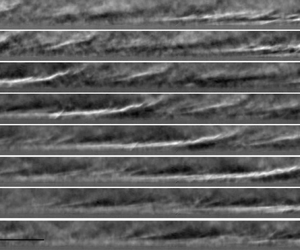
Figure 8. Enhanced schlieren visualizations showing the evolution of a single second-mode wavepacket from experiment S3. The first image is recorded at time $t_{0}$, with subsequent images at $t_{0}+21.3\ \mathrm {\mu }{\rm s}$, $t_{0}+42.6\ \mathrm {\mu } {\rm s}$ and $t_{0}+115.0\ \mathrm {\mu } {\rm s}$. The markers show the approximate extent of the wavepacket in the first image and have been translated downstream in the subsequent images according to the mean propagation speed.

Figure 9. Synthetic schlieren image computed using NPSE at the same free-stream conditions as experiment S3.

Figure 10. Wall-normal power spectral densities at times: (a) $t_{0}$, $R=1484$; (b) $t_{0}+21.3\ \mathrm {\mu } {\rm s}$, $R=1532$; (c) $t_{0}+42.6\ \mathrm {\mu } {\rm s}$, $R=1578$. (d) Structure angles of the wave fundamental frequency content at different points of development: (-$\Box$-) $t_{0}$; (-$\bigcirc$-) $t_{0}+21.3\ \mathrm {\mu } {\rm s}$; (-$\Diamond$-) $t_{0}+42.6\ \mathrm {\mu } {\rm s}$.

Next, we consider the inclination of the structures in the $s$–$y$ plane (often referred to as the structure angle), $\theta$, at different stages of development. The fundamental structure angle is calculated by first bandpass filtering the signal reconstructed at each wall-normal location around the fundamental second-mode frequency. Cross-correlation coefficients for vertically separated signals are computed for various streamwise displacements, and the displacement corresponding to the highest-valued coefficient is used to find the value of $\theta$. The lower right panel of figure 10 presents structure angles computed for the wavepackets shown in figure 8. In general, the fundamental content of the waves is tilted slightly upstream into the flow in the near-wall region, then rapidly curves towards the direction of the flow moving closer to the boundary-layer edge. The two more mature wavepacket stages shown in the second and third images of figure 8 take on a similar profile, reaching a maximum angle of $110^{\circ }$–$120^{\circ }$ between $y/\delta =0.2\text {--}0.4$. The minimum angles lie in the range 9$^{\circ }$–$15^{\circ }$ near the edge of the boundary layer. Similar measurements by Kimmel & Kendall (Reference Kimmel and Kendall1991), Parziale (Reference Parziale2013) and Laurence et al. (Reference Laurence, Wagner and Hannemann2016) cite minimum angles in the $10^{\circ }$–$15^{\circ }$ range.

4.1. Second-mode dominated regime

For cone configurations with nose-tip radii of 1.524 mm and less, the same temporal reconstruction technique as used in the sharp-nose case is applied and a similar analysis is performed. Sample images from experiments B1 and B2 are shown in figure 11. In figure 12 we show the most-amplified second-mode frequencies and their associated $N$ factors for experiments B1 and B2. Beginning with experiment B1, the frequencies computed by the LPSE are observed to be 10–20 % higher than the PCB and schlieren frequencies across the entire measurement range. Good agreement is observed between the PCB and schlieren measurements in the upstream portion of the visualization region. In the linear-growth regime, the slope of the $N$-factor curve computed from the schlieren is within 15 % of that computed from the LPSE. Deviation from the linear curve occurs at approximately $R=1820$ for both the schlieren and PCB measurements, resulting in a transition $N$ factor of 6.2. The higher transition $N$ factor here compared with the sharp-nose results is believed to be a combination of the higher unit-Reynolds-number free stream and higher most-amplified second-mode frequencies. Longer wavelength features similar to those observed by Casper et al. (Reference Casper, Beresch, Henfling, Spillers, Pruett and Schneider2016) in schlieren visualizations over a 7$^{\circ }$ half-angle cone in a Mach-5 free stream also appear. Casper et al. (Reference Casper, Beresch, Henfling, Spillers, Pruett and Schneider2016) attributed these low frequency disturbances to the first mode, and, considering the edge Mach numbers of 3.4–3.7 in the present experiments, it may be expected to be present to some extent here as well. While the direct numerical simulations (DNS) of Hader, Deng & Fasel (Reference Hader, Deng and Fasel2021) found the first mode to influence the transition process on a sharp-nose cone at Mach 5, a bispectral analysis of the present experiments did not indicate any significant nonlinear interactions between the lower-frequency and second-mode content. Turning to the results of experiment B2 (right plots of figure 12), a significant discrepancy is observed between the LPSE frequencies and those measured from the PCB and schlieren data. The greatest deviation between the LPSE and PCB measurements is observed upstream where the maximum frequency is difficult to extract due to the PCB signal being weak, while downstream the PCB and schlieren frequencies are roughly within 10 % of those of the LPSE. Additionally, the PCB sensors have a resonant frequency at roughly 300 kHz making identification of the peak frequency in the upstream sensors difficult. The reduced value of the measured frequencies compared with the computed frequencies is expected due to the finite initial amplitudes of the experimentally measured waves. The low signal-to-noise ratio in the upstream portion of the viewing area hindered the ability to compute $N$ factors from the schlieren measurements, but the PCB data agree well with the computation in figure 12(d).

Figure 11. Enhanced schlieren visualizations generated by subtracting a mean flow-on image from the image of interest. Images correspond to nose-tip-radius configurations of (a) 0.508 mm, (b) 1.524 mm.

Figure 12. (a,c) Experiment B1. (b,d) Experiment B2. (a,b) Most-amplified second-mode frequencies. (c,d) Plots of $N$ factors. Filled symbols are schlieren measurements; open symbols are PCB measurements; lines are LPSE results.

4.2. Non-modal instability features

The unsteady elongated features first appear consistently in the visualizations of the 2.54 mm nose-tip-radius configuration as shown in figure 13, and are frequently present for the 5.08 mm configuration. The following characterization focuses on the latter case as the features are significantly more visible due to both the image magnification and viewing location. For both experiments with this nose-tip bluntness (B4 and B5), the predicted entropy-layer swallowing length is roughly 1.25 m past the end of the cone model, and no significant difference in visual structure is observed between the features of the two slightly different experimental conditions. In general, the features extend above the visual edge of the boundary layer and are similar in appearance to those captured in the images of Grossir et al. (Reference Grossir, Pinna and Chazot2019). In contrast to the conditions where second-mode waves are present, no sharp peaks appear in the PCB power spectra computed over the entire test time; however, as seen in figure 14, isolated bursts of high-frequency (150–250 kHz) pressure content appear in the PCB signals resulting in a broad peak in the mean frequency spectra shown in figure 15. The peaks observed at approximately 300 kHz are most likely artifacts of the resonant frequency of the PCB sensors, and the spectra of the signals measured by the sensor at $s=341\ {\rm mm}$ contain significant noise at frequencies greater than 200 kHz. By matching the timestamps between the images and PCB array, it is possible to unambiguously associate the visible non-modal features with the high-frequency bursts in the PCB signals.

Figure 13. Enhanced schlieren visualization generated by subtracting a mean flow-on image from the image of interest for the 2.540 mm nose-tip-radius configuration.

Figure 14. Short-time Fourier transforms computed from PCB signals at (a) $s=241\ {\rm mm}$, (b) $s=341\ {\rm mm}$ for experiment B4.

Figure 15. Mean spectra computed from PCB signals for (a) experiment B4, (b) experiment B5.

General observations are made by analysing 15 clearly visible non-modal features present for experiments B4 and B5. These features develop slowly when compared with the rapid growth and breakdown of the second-mode instability waves. In presenting typical characteristics, we first consider the overall shape of such features. Focusing on figures 16 and 17, they are nearly parallel to the cone surface at the trailing (i.e.  upstream in the mean flow) edge and then gradually curve away from the surface. As the features propagate across the visualization region, the portion at the leading edge rotates downward towards the cone surface, resulting in a decrease in the inclination angle and flattening of the structure. The maximum inclination angle lies between 13$^{\circ }$–$19^{\circ }$ when the feature is at the most upstream end of the viewing area and decreases to 8$^{\circ }$–$14^{\circ }$ once it has propagated to the most downstream visible location. Figure 18 shows this evolution in feature shape by presenting the profile of maximum pixel intensity within a single non-modal feature at four sequential timesteps (separated by $21.3\ \mathrm {\mu }{\rm s}$) from experiment B4. Select features such as that shown in figure 16(h) are also observed to exhibit a region of high curvature near the leading edge (downstream end). In general, the features extend $2\delta -3\delta$ above the cone surface, and the strongest density gradients are observed at a wall-normal height of $1\delta -2.5\delta$. The linear non-modal analysis of planar waves of the B4 configuration is shown in figure 19. The linearly optimal perturbations that result in maximum Mack's energy gain, $G_{E}$, at a specified downstream location are computed with the variational formulation based on the HLNSE (Paredes et al. Reference Paredes, Choudhari, Li, Jewell and Kimmel2019b). The inflow location is selected at $s_0=24\ {\rm mm}$, close to the nose-tip juncture. Figure 19(a) shows the dependency of the optimization outflow location with respect to the disturbance frequency for maximum energy gain. Figure 19(b) shows the optimal energy gain in terms of the $N$ factor calculated as $N_E=0.5\log (G_E)$, corresponding to the outflow locations for maximum energy growth of figure 19(a) for the selected frequencies. The outflow location and disturbance frequencies that correspond to the maximum energy gain are $s_1=305\ {\rm mm}$ and $f=125\ {\rm kHz}$. The corresponding inflow disturbance profile with the parameters corresponding to maximum energy gain (i.e. $s_0=24\ {\rm mm}$, $s_1=305\ {\rm mm}$ and $f=125\ {\rm kHz}$) is used as the inflow condition for the parabolic integration of the NPSE with an initial amplitude of $|T'|_{rms}/T_\infty =0.002$. The synthetic schlieren image of the disturbance is shown in figure 20. Comparison of DNS and NPSE results of the nonlinear evolution of non-modal waves in a blunt cone was presented by Paredes et al. (Reference Paredes, Choudhari and Li2020). As observed by comparing figures 17 and 20, the individual experimental and computation features are very similar in appearance and share, for example, the gradual flattening of the structure with downstream propagation, indicating that they are likely the same features. While the spatial periodicity of the features in figure 20 is not apparent in figure 17, this is not necessarily expected in the experimental measurements as the $N$ factor is fairly flat over a wide range of frequencies in figure 19(b) and the computations of Paredes et al. (Reference Paredes, Choudhari, Li, Jewell, Kimmel, Marineau and Grossir2019c) predict the non-modal features to exhibit amplification over a broad range of frequencies. The inclination angles of the computed features lie slightly below the lower end of the experimentally observed range with values of approximately 11$^{\circ }$ and 7$^{\circ }$ at the most upstream and downstream streamwise locations.

Figure 16. Enhanced visualization sequence from experiment B4 ($R_{N}=5.08\ {\rm mm}$). The top image corresponds to time $t_{0}$ with subsequent images separated by $21.3\ \mathrm {\mu } {\rm s}$ (i.e.  every fifth image shown). Black arrows indicate the streamwise locations of the three most downstream PCB sensors ($s=291$ mm, $s=316\ {\rm mm}$ and $s=341\ {\rm mm}$). The black horizontal line in the final image indicates the computed boundary-layer thickness.

Figure 17. Enhanced visualization sequence from experiment B5 ($R_{N}=5.08\ {\rm mm}$). The top image corresponds to time $t_{0}$ with subsequent images separated by $21.3\ \mathrm {\mu } {\rm s}$ (i.e.  every fifth image shown). Black arrows indicate the streamwise locations of the three most downstream PCB sensors ($s=291$, $s=316$ and $s=341\ {\rm mm}$). The black horizontal line in the final image indicates the computed boundary-layer thickness.

Figure 18. Profile of maximum pixel intensity extracted for the feature shown in images (i)–(l) of figure 16.

Figure 19. Characteristics of the optimal perturbation used as the inflow condition for the NPSE calculations. (a) Outflow location ($s_1$) for maximum energy gain disturbance frequency; (b) $N$ factor computed using the Mack energy norm versus disturbance frequency. The circle indicates the maximum $N_{E}$.

Figure 20. Synthetic schlieren computed for the same free-stream conditions as experiment B5. The white horizontal line indicates the computed boundary-layer thickness.

In figure 21 we show the streamwise PCB pressure traces corresponding to the image sequences presented in figures 16 and 17. Two distinct instability features are observed in the lower unit-Reynolds-number experiment B4 shown in figure 16; their associated pressure footprints are seen in the most upstream PCB sensor at $t-t_{0}=95\ \mathrm {\mu } {\rm s}$ and $t-t_{0}=240\ \mathrm {\mu } {\rm s}$. As the feature passes over the sensor, a slight rise followed by several high-frequency (several hundred kHz) oscillations is characteristic of the pressure disturbance at the wall; a similar pressure disturbance with a frequency of approximately 250 kHz is observed in the most upstream sensor for the experiment B5 disturbance. The two disturbances for experiment B4 in the left plot of figure 21 have a similar profile until $s=316\ {\rm mm}$, by which point the high-frequency content in the earlier disturbance has been significantly amplified and that of the later disturbance attenuated. By $s=341\ {\rm mm}$, the earlier disturbance contains extremely strong content with a frequency of approximately 182 kHz, and the later disturbance is almost completely attenuated. The rapid amplification of the earlier disturbance recorded at the two most downstream sensors is an anomalous case; all other pressure disturbances associated with non-modal features appear similar in shape and magnitude up through the sensor at $s=291\ {\rm mm}$ and see minimal amplification in the more downstream sensors. Nonetheless, this unique disturbance is worth noting, as it appears visually similar to the other instability features and no obvious high-frequency signal appeared in the schlieren images corresponding to these features. In general, the high-frequency pressure disturbances generated by the non-modal features of experiment B5 exhibit slightly higher frequencies than those of experiment B4. Given the inversely proportional relationship between the second-mode fundamental frequencies and boundary-layer thickness, this may indicate that the high-frequency pressure disturbances associated with the trailing edge of the non-modal features are related to the second mode.

Figure 21. Plots of PCB pressure traces at different streamwise locations: (a) experiment B4, (b) experiment B5. The traces are vertically offset according to the measurement coordinate.

In figure 22 we show the pressure signals recorded by the PCB spanwise array during the time period of the two image sequences. The circumferential extent of the high-frequency pressure disturbance appears limited, typically encompassing just two of the laterally offset sensors with minimal content at the third. Beginning with B4, the high-frequency disturbance at $t-t_{0}=200\ \mathrm {\mu } {\rm s}$ is strongest in the centre sensor, with a weak pressure disturbance present in the sensors located on either side at $\zeta =5.72\ {\rm mm}$ and $\zeta =-5.72\ {\rm mm}$ (though this was an exceptional case). Weak content is also observed in the $\zeta =-5.72\ {\rm mm}$ and $\zeta =0$ sensor signals at $t-t_{0}=50\ \mathrm {\mu } {\rm s}$ and $t-t_{0}=340\ \mathrm {\mu } {\rm s}$. For the B5 traces, the pressure disturbance at time $t-t_{0}=110\ \mathrm {\mu } {\rm s}$ is visible in both the $\zeta =-5.72\ {\rm mm}$ and $\zeta =0$ sensor, but minimal signature is observed in the $\zeta =5.72\ {\rm mm}$ sensor. For both experiments, the maximum coherence over all frequencies gives a magnitude-squared coherence estimate of 0.4–0.55 for adjacent sensors. Limited coherence ($\sim$0.1) is observed between the $\zeta =-5.72\ {\rm mm}$ and $\zeta =5.72\ {\rm mm}$ sensor signals, though ambiguity remains in defining the features associated with non-modal growth using solely the pressure data because of the lack of a single distinguishing disturbance frequency. In terms of the local boundary-layer thickness computed from the DPLR mean-flow solution, the resulting spanwise extent of the high-frequency disturbances is of the order of $5\delta -10\delta$.

Figure 22. Plots of PCB pressure traces at different spanwise locations: (a) experiment B4, (b) experiment B5. The traces are vertically offset according to the measurement coordinate.

Propagation speeds are computed by selecting a region of the feature located between the boundary-layer and entropy-layer edges and using a cross-correlation technique to identify the downstream propagation between sequential images, similar to calculations of the second-mode propagation speeds. The average speed and 95 % confidence interval calculated over 162 image pairs from experiment B4 is $780\pm 90.1\ {\rm m}\ {\rm s}^{-1}$; values calculated for experiment B5 also fall within this range. The edge velocities computed for these two conditions using the DPLR mean-flow solution are $761\ {\rm m}\ {\rm s}^{-1}$ and $757\ {\rm m}\ {\rm s}^{-1}$, respectively, leading to a $u_{prop}/u_{e}=1.03$. Slightly higher propagation velocities are expected given that the structures extend beyond the boundary-layer edge. Additionally, no clear regularity is observed in the spacing between features. We can identify two possibilities for this lack of clear frequency content: the instability features undergoing non-modal amplification are not associated with a single dominant frequency, or the reduced schlieren contrast resulting from the entropy layer combined with the integrated nature of the technique eliminates the ability to consistently identify features. A dominant disturbance frequency may, however, not be expected as the computational results of Paredes et al. (Reference Paredes, Choudhari, Li, Jewell and Kimmel2019b) predict that the non-modal features exhibit amplification over a significantly broader range of frequencies than the second mode, with the most-amplified frequencies lying in the 100–800 kHz range depending on the cone model nose-tip radius and free-stream conditions. Free-stream noise levels may also play a role in which frequency disturbances become most amplified.