


1. Introduction
Taylor–Couette flow (TCF) refers to the annular flow between two concentric, differentially rotating cylinders. Following the seminal work of Taylor (Reference Taylor1923) that clarified the stabilizing effect of viscosity on the onset of Taylor vortices, there have been numerous experimental, numerical and theoretical investigations on TCF (Taylor Reference Taylor1936a,Reference Taylorb; Velikhov Reference Velikhov1959; Chandrasekhar Reference Chandrasekhar1960; Coles Reference Coles1965; Synder Reference Synder1968; Gollub & Swinney Reference Gollub and Swinney1975; Cole Reference Cole1976; Benjamin Reference Benjamin1978a,Reference Benjaminb; Mullin & Benjamin Reference Mullin and Benjamin1980; DiPrima & Swinney Reference DiPrima and Swinney1981; Jones Reference Jones1981; Cliffe Reference Cliffe1983; Marcus Reference Marcus1984; Andereck, Liu & Swinney Reference Andereck, Liu and Swinney1986; Pfister et al. Reference Pfister, Schmidt, Cliffe and Mullin1988; Nakamura et al. Reference Nakamura, Toya, Yamashita and Ueki1989) during the last century. The majority of the theoretical and numerical studies were done for the ideal case of infinite cylinders, numerically implemented by enforcing periodic boundaries along the axial direction, including the viscous stability analysis of Taylor (Reference Taylor1923). It is now well known that the azimuthally invariant stationary axial-roll solutions, called Taylor vortices, bifurcate from the purely azimuthal base state of the circular Couette flow (CCF), via a supercritical pitchfork bifurcation (Taylor Reference Taylor1923; Chandrasekhar Reference Chandrasekhar1961), beyond a minimum speed of the inner cylinder. In a finite length Taylor–Couette cell with rigid lids, because of no-slip boundary conditions, the velocity near the top and bottom walls drops to zero where the centrifugal force is weaker in comparison with that at the midheight of the container. Hence, the flow near the top and bottom is expected to be radially inwards, while at the midplane the flow is expected to be radially outwards. Figure 1(a) shows a schematic of the midplane symmetric Taylor-vortices that are normally observed in TCF.

Figure 1. (a) Schematic of ‘normal’ Taylor vortices, with inward jets near top and bottom walls. (b–d) Schematic of anomalous modes in the  $(r, z)$-plane: (b,c) single-roll or asymmetric 2-roll modes and (d) anomalous 2-roll mode.
In contrast to the canonical solution depicted in figure 1(a), however, the bifurcation scenario can be different in the realistic case of finite length cylinders with end plates. Since the end plates induce Ekman vortices at finite rotation of cylinders, the CCF state is not strictly realizable in axially bounded TCF. With the discovery of the so-called ‘anomalous’ modes by Benjamin (Reference Benjamin1978a,Reference Benjaminb), many experimental and numerical investigations have confirmed the existence of these modes in incompressible TCF over the last 40 years (Schaeffer Reference Schaeffer1980; Benjamin & Mullin Reference Benjamin and Mullin1981, Reference Benjamin and Mullin1982; Hall Reference Hall1982; Cliffe Reference Cliffe1983; Lücke et al. Reference Lücke, Mihelcic, Wingerath and Pfister1984; Jones Reference Jones1985; Bolstad & Keller Reference Bolstad and Keller1987; Pfister et al. Reference Pfister, Schmidt, Cliffe and Mullin1988; Nakamura et al. Reference Nakamura, Toya, Yamashita and Ueki1989; Youd & Barenghi Reference Youd and Barenghi2005), with the most recent work being reported by Mullin, Heise & Pfister (Reference Mullin, Heise and Pfister2017). Anomalous modes is a general term which includes Taylor-like vortices that are symmetric about the midplane but have the opposite sense of rotation (compared with a ‘normal’ Taylor vortex mode in figure 1a), i.e. the flow is radially inward at midheight and outward near the top and bottom walls. There is also a possibility of odd numbered rolls, which break the midplane symmetry. Figure 1(b–d) shows a schematic of the flow directions in three representative cases of anomalous modes; the bolder arrows represent stronger rolls, while the weaker rolls can be seen near the top and/or bottom walls in each panel. In the small aspect ratio limit of  $\varGamma = h/\delta \sim O(1)$ (where
  $h$ is the height of the cylinders and
  $\delta =R_o-R_i$ is the gap width), the asymmetric two-vortex modes (figure 1b,c, also called the single-roll modes) have been observed. Apart from the aspect ratio
  $\varGamma =h/\delta$, the other control parameter for the TCF is the inner Reynolds number,
 \begin{equation} Re_i = \frac{\rho_R \varOmega_i R_i \delta}{\mu_R}, \end{equation}
where  $\rho _{R}$ and
  $\mu _{R}$ are reference density and viscosity scales,
  $\varOmega _{i}$ is the angular velocity of the inner cylinder; it is assumed that the outer cylinder is kept stationary (
 $\varOmega _o=0$) as in the experiments of Benjamin (Reference Benjamin1978b) as well as in most subsequent studies on anomalous modes in TCF.
In a detailed experimental and theoretical investigation, Benjamin (Reference Benjamin1978a,Reference Benjaminb) discovered that the anomalous Taylor vortices can appear via imperfect pitchfork bifurcations. Benjamin & Mullin (Reference Benjamin and Mullin1981) confirmed the existence of such anomalous modes over a broad a range of parameters, leading to phase diagrams in the ( ${Re}, \varGamma$)-plane, delineating the phase boundaries between anomalous and normal Taylor vortices. Schaeffer (Reference Schaeffer1980) proposed a reduced-order model to explain the hysteresis phenomenon observed in Benjamin's experiments – he used a homotopy parameter which connected the periodic boundary conditions modelling infinite cylinders to the no-slip case in a finite domain with stationary top and bottom lids which mimics experiments; Hall (Reference Hall1982) studied Schaeffer's model in a quantitative manner. Cliffe (Reference Cliffe1983) used a finite element method in combination with numerical bifurcation techniques to implement the mathematical framework of Schaeffer (Reference Schaeffer1980) that helped to relate nonlinear solutions in an axially periodic TCF with those in its axially bounded counterpart – in particular, he confirmed the experimental finding of the ‘single-roll’ mode of Benjamin & Mullin (Reference Benjamin and Mullin1981). Note that for the single-roll mode depicted in figure 1(b,c), there exist two rolls which are not midplane symmetric, one of the rolls is bigger and is located near the top or the bottom wall and there exists another roll of the opposite circulation, but it is weaker in comparison to the bigger roll. Similarly for anomalous modes that are mirror symmetric about the midplane (see figure 1d), there exist two weaker rolls near the top and bottom walls which are difficult to observe in experiments. Bolstad & Keller (Reference Bolstad and Keller1987) used the multigrid method along with pseudo-arclength continuation to compute anomalous modes in TCF; their computations also provided evidence of weaker rolls near the top and bottom walls that might not be discernible in experiments. Benjamin & Mullin (Reference Benjamin and Mullin1982) reported multiple solutions for the same values of the aspect ratio
  $\varGamma$ and the inner Reynolds number
  $Re$. Later experiments by Mullin (Reference Mullin1982) uncovered mutations of Taylor-like vortices where he identified the cusp catastrophe (Zeeman Reference Zeeman1976) in the (
 $\varGamma , Re$)-plane.
In addition to the multiplicity of steady Taylor rolls, the time-dependent wavy jet patterns have been identified by Mullin & Benjamin (Reference Mullin and Benjamin1980) and Lorenzen, Pfister & Mullin (Reference Lorenzen, Pfister and Mullin1982) in experiments with small aspect ratio  $\varGamma =O(5)$ Taylor–Couette (TC) cell, and verified in Navier–Stokes simulations by Jones (Reference Jones1985). Furukawa et al. (Reference Furukawa, Watanabe, Toya and Nakamura2002) numerically studied the transient problem of TCF over a range of aspect ratios between
  $0.5$ to
  $1.6$ for a radius ratio of
  $2/3$; along with the normal two-cell mode, anomalous one-cell mode and a twin-cell mode (a new time-dependent mode) were observed in their numerical study. In the experimental-cum-numerical study, Mullin, Toya & Tavener (Reference Mullin, Toya and Tavener2002) found that the symmetry-breaking bifurcation sequences merge in a self-consistent way when the aspect ratio is reduced so that for very small aspect ratios, only midplane symmetric steady flows exist. Recently, Cliffe, Mullin & Schaeffer (Reference Cliffe, Mullin and Schaeffer2012) studied the role of approximate symmetry on the onset of rolls in the finite cylinder case; they attributed the sharp onset of Taylor vortices in long but finite cylinders to the fact that for large number of cells (
 $k$), the flows with
  $2k$- and
  $2(k+1)$-number of cells are similar to one another. Most recently, Mullin et al. (Reference Mullin, Heise and Pfister2017) provided experimental evidence supporting the above hypothesis. For a recent review on TCF, we refer to Grossmann, Lohse & Sun (Reference Grossmann, Lohse and Sun2016) and to Barkley (Reference Barkley2016) for related issues from the perspectives of finite-amplitude nonlinear states and dynamical systems theory.
All above works dealt with incompressible TCF. However, not much work, be it experimental (Kuhlthau Reference Kuhlthau1949, Reference Kuhlthau1960), theoretical or numerical, has been done on its compressible counterpart. Kuhlthau (Reference Kuhlthau1960) conducted a series of experiments on compressible TCF with the low-density air as the working fluid. The inner cylinder was rotated, with two end plates being tied to the stationary outer cylinder; the experiments were carried out for two aspect ratios of  $\varGamma =5$ and
  $6.2$, respectively, with radius ratios of
  $\eta =0.8$ and
  $0.89$. He reported torque data, measured on the outer cylinder, as a function of the pressure that spanned over a range of Mach numbers
  $0.37 \leq {Ma} \leq 1.47$; note that Mach number was estimated based on the gas properties at the surface of the rotating inner cylinder. The primary results of these experiments are as follows: the onset of transition to Taylor vortices (tied with increased torque) is delayed with (i) increasing
  $Ma$ and (ii) decreasing the annular gap-width.
On prior theoretical works on compressible TCF, Kao & Chow (Reference Kao and Chow1992) carried out a linear stability analysis by assuming axisymmetric disturbances, with a radius ratio  $\eta = {R_i}/{R_o} = 0.5$. Their results apparently implied that increasing Mach number (
 $Ma$) destabilized the flow, in contradiction with the experiments of Kuhlthau (Reference Kuhlthau1960). On the other hand, the linear stability analyses of Hatay et al. (Reference Hatay, Biringen, Erlebacher and Zorumski1993) concluded that increasing
  $Ma$ stabilizes the flow for narrow gaps (
 $\eta > 0.8$) and destabilizes it for wide gaps. Note that both Kao & Chow (Reference Kao and Chow1992) and Hatay et al. (Reference Hatay, Biringen, Erlebacher and Zorumski1993) defined the Reynolds number based on the local density which led to ‘incorrect’ conclusions about the role of compressibility on the onset of centrifugal instabilities as explained below. Since the variation between local and average densities can be quite large at large supersonic speed, using the critical Reynolds number based on the local density is not a correct measure as pointed out by Manela & Frankel (Reference Manela and Frankel2007). For this reason, the stabilizing or destabilizing effect of increasing
  $Ma$ might not be unequivocal. Manela & Frankel (Reference Manela and Frankel2007) focused on the narrow-gap limit, conducted a linear stability analysis and correctly concluded that increasing
  $Ma$ stabilizes the flow, confirming the experimental results of Kuhlthau (Reference Kuhlthau1960). Most recently, Welsh, Kersal'e & Jones (Reference Welsh, Kersal'e and Jones2014) carried out a linear stability analysis for the TCF for a wide-gap case, with a radius ratio of
  $\eta = {R_i}/{R_o} = 0.5$ and they also confirmed stabilizing effect of compressibility on the onset of Taylor-vortices. At high Prandtl numbers, they found new instability modes that become unstable to oscillatory axisymmetric disturbances. Interestingly, they also reported the onset of instability even when the angular momentum increases outwards, which implies that the classical Rayleigh criterion can be violated in the compressible TCF. To understand the fate of the above mentioned linear instability modes in the nonlinear Taylor-vortex regime, the direct numerical simulations of compressible Navier–Stokes equations must be carried out, which has not yet been done for compressible TCF. Recently, Gopan & Alam (Reference Gopan and Alam2020) analysed the TCF of a ‘dense’ gas using molecular dynamics simulations, but the roles of (i) gas compressibility and (ii) the end-wall conditions have not been analysed systematically.
In this work, we employ direct numerical simulations to understand the role of compressibility on the ‘ $2k\mathop \leftrightarrow \limits^{{\rm rolls}} 2(k + 1)$’-roll transition and the onset of asymmetric (anomalous) modes in ‘axially bounded’ compressible TCF of a dilute gas in the wide-gap limit. As a first step, we leave aside certain non-continuum effects (slip velocity, rarefaction, etc.) and focus primarily on the effect of fluid compressibility on pattern transitions as (i) the inner-cylinder Reynolds number and (ii) the heights of the cylinders are varied. In particular we ask: How does the gas compressibility affect the bifurcation scenario and pattern transition in finite-cylinder compressible TCF? Following the experimental protocols of Benjamin (Reference Benjamin1978b), we vary the height of the cylinders quasistatically in numerical simulations and analyse transitions among different-numbered Taylor rolls as functions of (
 ${Re}, \varGamma$).
This paper is organized as follows. Choosing the ideal gas as a working fluid, the compressible Navier–Stokes–Fourier equations (see § 2) are numerically solved using direct numerical simulation with an in-house finite-difference code, the details of which are documented in appendix A of the supplementary material available at https://doi.org/10.1017/jfm.2020.897. The Taylor–Couette system is bounded axially by two non-rotating end plates, with only the inner cylinder rotating ( $\varOmega _i\neq 0$ and
  $\varOmega _o = 0$); the no-slip condition enforced at the end plates ensures the presence of two Ekman vortices at any finite value of
  $\varOmega _i$. The results on ‘
 $2k\rightarrow 2(k+1)$’-roll transition and the role of Mach number are analysed in § 3. The anomalous single-roll (i.e. asymmetric 2-roll) mode, the phase diagram of
  $1\mathop \leftrightarrow \limits^{{\rm rolls}} 2$ transition, the related bifurcation diagrams and the non-trivial role of compressibility are discussed in § 4. A summary of results with conclusions and possible future works are provided in § 5. Additional details are provided in appendices A and B that are relegated to the supplementary materials.
2. Governing equations and numerical method
Figure 2 shows a schematic of the Taylor–Couette set-up, with ( $r, \phi , z$) denoting the radial, azimuthal and axial coordinates. Let
  $\rho ^*$,
  $T^*$ and
  $p^*$ be the local density, temperature and pressure of the gas, respectively, and
 \begin{equation} \boldsymbol{u^{*}} \equiv (u_r, u_\phi, u_z) =(u, v, w) \end{equation}
be the velocity vector (with radial, azimuthal and axial velocity components denoted by  $u$,
$u$,  $v$ and
  $w$, respectively), with the superscript
  $*$ referring to dimensional quantities. The governing equations are the well known compressible Navier–Stokes equations, coupled with mass conservation and Fourier/energy equations, and the equation of state is taken to be that of an ideal gas:
  $p^{*}=(c_{p}^{*}-c_{v}^{*})\rho ^{*} T^{*}$, where
  $c_p^{*}$ and
  $c_v^{*}$ are specific heats at constant pressure and volume, respectively, and
  $\gamma =c_p^*/c_v^*$ is the ratio of specific heats (Liepmann & Roshko Reference Liepmann and Roshko1961; Chapman & Cowling Reference Chapman and Cowling1970). The reference scales used to make these equations dimensionless are shown in table 1.

Figure 2. (a) Geometry of the finite-cylinder TCF with rigid lids at top and bottom; the inner and outer cylinders of radii  $R_i$ and
  $R_o$, respectively, with length of
  $h$ have rotation rates of
  $\varOmega _i$ and
  $\varOmega _o$. (b) Schematic of the
  $(r, z)$-plane with dimensionless boundary conditions; the inner and outer cylinders are maintained at the same temperature,
  $T(r=R_i) =T_i/T_i=1$ and
  $T(r=R_o) =T_o/T_i=\chi =1$.
Table 1. Various reference scales:  $\delta =R_o-R_i$ is the annular gap width and
  $M_{t}$ is the mass of the fluid per unit length in the annular region; the reference temperature
  $T^{*}|_{R_{i}}$ is evaluated at the inner cylinder;
  $c_{p}^{*}$ and
  $c_{v}^{*}$ are specific heats at constant pressure and volume, respectively; the reference viscosity
  $\mu ^{*}_R$ as well as the thermal conductivity
  $\kappa ^{*}_R$ of the gas are taken to be constant.

The dimensionless forms of mass, momentum and energy equations are given by
 \begin{gather} \frac{\partial \rho}{\partial t}+\boldsymbol{\nabla}\boldsymbol{\cdot} (\rho\boldsymbol{u})=0, \end{gather}
 \begin{gather}\frac{{\mathcal{D}} (\rho u_\alpha)}{{\mathcal{D}} t} = - \frac{Re_{i}^{2}}{Ma^{2}}\boldsymbol{\nabla} p + \left[\nabla^{2}\boldsymbol{u}+\frac{1}{3}\frac{\partial}{\partial x_\alpha}(\boldsymbol{\nabla} \boldsymbol{\cdot} \boldsymbol{u})\right], \end{gather}
 \begin{gather}\frac{{\mathcal{D}} (\rho T)}{{\mathcal{D}} t} = -(\gamma - 1)p (\boldsymbol{\nabla} \boldsymbol{\cdot} \boldsymbol{u}) + \frac{\gamma}{Pr} \nabla^{2}T + \frac{(\gamma -1) Ma^{2}}{Re_i^{2}}\varPhi, \end{gather}
where
 \begin{equation} \frac{{\mathcal{D}} \psi}{{\mathcal{D}} t} = \frac{\partial \psi}{\partial t} + \boldsymbol{\nabla} \boldsymbol{\cdot} [\boldsymbol{u} \psi] \end{equation}
for some physical quantity  $\psi$, and the equation of state in dimensionless form is
  $p = \rho T$. In the energy equation (2.2c), the viscous dissipation term is given by
 \begin{equation} \varPhi = 2\mu D_{\alpha\beta} D_{\alpha\beta} + \lambda(\boldsymbol{\nabla}\boldsymbol{\cdot}\boldsymbol{u})^2, \end{equation}
where  ${\boldsymbol D}=({\boldsymbol \nabla }{\boldsymbol u} + ({\boldsymbol \nabla }{\boldsymbol u})^\dagger )/2$ is the symmetric part of the velocity gradient tensor. Throughout this work, we use the Stokes assumption of zero bulk viscosity (Liepmann & Roshko Reference Liepmann and Roshko1961; Malik, Alam & Dey Reference Malik, Alam and Dey2006; Malik, Dey & Alam Reference Malik, Dey and Alam2008), i.e.
  $\xi = \lambda + {2 \mu }/{3} = 0$, resulting in an expression for the second viscosity in terms of the shear viscosity,
  $\lambda = - {2 \mu }/{3}$ that holds strictly for a monatomic gas (Chapman & Cowling Reference Chapman and Cowling1970).
Apart from inner-cylinder Reynolds number  ${Re}$, there are two additional dimensionless numbers that appear in (2.2), namely the Mach number
  $Ma$ and the Prandtl number
  $Pr$. The Reynolds numbers based on the angular velocities of inner and outer cylinders is defined via (1.1), with
  $Re_i>0$ and
  $Re_o=0$ for all calculations in this work. The Mach number, based on the rotational speed of the inner cylinder, is defined as
 \begin{equation} Ma = \frac{\varOmega_iR_i}{c_s^*} = \frac{Re}{c_s}, \end{equation}
where  $c_s= \sqrt {(c_p^* -c_v^*){\rho ^*_R}^2 T^{*}_R \delta ^{2}/{\mu ^*_R}^2}$ is the dimensionless ‘isothermal’ sound speed (based on the gas properties at the inner cylinder),
  $Re=Re_i$ is the inner-cylinder Reynolds number (1.1) and the Prandtl number is
  $Pr = \mu ^* c_p^*/\kappa ^*$. There are two geometric parameters, namely the aspect ratio
  $\varGamma =h/\delta$ and the radius ratio
  $\eta =R_i/R_o$ of the TC-cell.
2.1. Axisymmetric TCF and boundary conditions
Focussing on the axisymmetric case ( $\partial /\partial \phi (\cdot )=0$), we multiply the governing equations (2.2a)–(2.2c) by
  $r$ throughout. The resulting continuity,
  $r$-momentum,
  $\phi$-momentum,
  $z$-momentum and energy equations are then rewritten as
 \begin{equation} \frac{\partial \bar{\rho}}{\partial t}+\frac{\partial}{\partial r}(\bar{\rho} u)+ \frac{\partial}{\partial z}(\bar{\rho}w)=0, \end{equation}
 \begin{align} & \frac{\partial (\bar{\rho} u)}{\partial t} + \frac{\partial}{\partial r} [ u (\bar{\rho} u)] + \frac{\partial}{\partial z}[w(\bar{\rho} u)] -\frac{\bar{\rho} v^{2}}{r} \nonumber\\ &\quad =-\frac{Re_{i}^{2}}{Ma^{2}}\left( r \frac{\partial p}{\partial r}\right) + r\left[\left( \frac{\partial^{2} u}{\partial r^{2}}+\frac{\partial^{2} u}{\partial z^{2}} + \frac{\partial}{\partial r}\left(\frac{u}{r}\right)\right) + \frac{1}{3} \frac{\partial}{\partial r}\left( \frac{1}{r}\frac{\partial}{\partial r}(r u)+ \frac{\partial}{\partial z}(w)\right)\right], \end{align}
 \begin{equation} \frac{\partial (\bar{\rho} v)}{\partial t}+\frac{\partial}{\partial r} [u (\bar{\rho} v)]+ \frac{\partial}{\partial z}[w(\bar{\rho} v)]+\frac{\bar{\rho} uv}{r} = r\left[\left(\frac{\partial^{2} v}{\partial r^{2}}+\frac{\partial^{2} v}{\partial z^{2}} + \frac{\partial}{\partial r}\left(\frac{v}{r}\right)\right)\right], \end{equation}
 \begin{align} & \frac{\partial (\bar{\rho} w)}{\partial t}+ \frac{\partial}{\partial r} [u(\bar{\rho} w)]+ \frac{\partial}{\partial z}[w(\bar{\rho} w)] \nonumber\\ &\quad =-\frac{Re_{i}^{2}}{Ma^{2}}\left( r \frac{\partial p}{\partial z}\right) + r\left[\left(\frac{\partial^{2} w}{\partial r^{2}}+\frac{\partial^{2} w}{\partial z^{2}} + \frac{1}{r}\frac{\partial w}{\partial r} \right) +\frac{1}{3} \frac{\partial}{\partial z} \left( \frac{1}{r}\frac{\partial}{\partial r}(r u)+\frac{\partial}{\partial z}(w)\right)\right], \end{align}
 \begin{align} & \frac{\partial (\bar{\rho} T)}{\partial t}+\frac{\partial}{\partial r} [ (\bar{\rho} u) T]+ \frac{\partial}{\partial z}[(\bar{\rho} w) T] \nonumber\\ &\quad =-(\gamma-1)p r\left( \frac{1}{r}\frac{\partial}{\partial r}(r u)+ \frac{\partial}{\partial z}(w)\right) +r\left[\frac{\gamma}{Pr} \left(\frac{1}{r}\frac{\partial}{\partial r}\left(r\frac{\partial T}{\partial r}\right)+ \frac{\partial^{2}T}{\partial z^{2}}\right)\right] \nonumber\\ &\qquad + r(\gamma -1)\frac{Ma^{2}}{Re_{i}^{2}}\left\{\left[2\left(\frac{\partial u}{\partial r}\right)^{2}+ 2\left(\frac{u}{r} \right)^{2}+2\left(\frac{\partial w}{\partial z}\right)^{2}+ \left(\frac{\partial v}{\partial r} -\frac{v}{r} \right)^{2} \right.\right.\nonumber\\ &\qquad \left.\left.+\left(\frac{\partial u}{\partial z}+\frac{\partial w}{\partial r}\right)^{2}+ \left(\frac{\partial v}{\partial z} \right)^{2}\right]-\frac{2}{3}\left[\frac{1}{r^{2}} \left(\frac{\partial (ru)}{\partial r} \right)^{2}+\left(\frac{\partial w}{\partial z}\right)^{2}+ \frac{2}{r}\frac{\partial (ru)}{\partial r}\frac{\partial w}{\partial z}\right]\right\}, \end{align}
where
 \begin{equation} \bar{\rho}=\rho r \end{equation}
is the rescaled density, and the equation of state is  $p=\bar {\rho } T/r$. Writing equations in this way (Harada Reference Harada1980) amounts to making the convective derivatives look as if (2.6a)–(2.6e) are written in Cartesian coordinates, which is advantageous for numerical discretization.
The boundary conditions are zero-slip at the cylinder walls as well as at stationary top and bottom lids,
 \begin{gather} u=w=0 \quad \textrm{at}\ r= \frac{\eta}{1-\eta} \quad \mbox{and} \quad r= \frac{1}{1-\eta}, \end{gather}
 \begin{gather}v=Re_i \quad \textrm{at}\ r= \frac{\eta}{1-\eta}, \quad v=Re_o \quad \textrm{at}\ r= \frac{1}{1-\eta}, \end{gather}
 \begin{gather}u=v=w=0 \quad \textrm{at}\ z=0 \quad \textrm{and} \quad \varGamma, \end{gather}
and the Dirichlet boundary conditions for temperature are
 \begin{equation} T=1 \quad \textrm{at}\ r= \frac{\eta}{1-\eta} \quad \mbox{and} \quad T=\frac{T_o}{T_i}=\chi \quad \textrm{at}\ r= \frac{1}{1-\eta}. \end{equation}
Note that the inner and outer cylinders are located at  $r=\eta /(1-\eta )$ and
  $1/(1-\eta )$, respectively, with
  $\eta =R_i/R_o$ being the radius ratio. The temperature ratio
  $\chi = T_o/T_i$ is taken to be
  $1$, unless stated otherwise, i.e. both cylinders are kept at the same temperature.
2.2. Numerical method and the code validation
A finite difference code has been developed to numerically solve (2.6) along with boundary conditions (2.8). The details of the numerical scheme (Harada Reference Harada1980) are documented in appendix A.1 (see supplementary material). To validate the present code, the onset of Taylor vortices with periodic boundary conditions along the axial direction was analysed.
The simulation data on the axial variation of the radial-averaged radial velocity, i.e.  $u(z) =\langle u(r,z)\rangle _r$, are shown in figure 3(a) for a range of inner-cylinder Reynolds number
  $Re$; the Mach number is set to
  $Ma=1$, the Prandtl number is
  $Pr=1$ and the aspect ratio of the TC-cell is
  $\varGamma =h/\delta =1.98$ with a radius ratio of
  $\eta =R_i/R_o=1/2$. For the idealized case of purely azimuthal CCF that occurs at small values of
  $Re$, the radial velocity is zero, see the blue horizontal line for
  $Re=71$ in figure 3(a). However, when the flow bifurcates to TVF, the radial velocity is non-zero due to presence of Taylor rolls, see the velocity profiles for
  $Re\geq 72$ in figure 3(a); the related velocity vectors and the streamline patterns at
  $Re=75$ are displayed in figures 3(c) and 3(d), respectively. To quantify bifurcation from CCF to TVF, the maximum of the radial-averaged radial velocity,
 \begin{equation} {\rm \Delta} u =max\, u(z), \end{equation}
is used as a metric. The variation of (2.9) with  $Re$ is shown in figure 3(b); the critical/minimum Reynolds number for the onset of Taylor rolls, extracted from figure 3(b) is
  $Re_{cr}\approx 71$ – this value is very close to
  $Re_{cr} = 71.635$ reported by Welsh et al. (Reference Welsh, Kersal'e and Jones2014) from the linear stability analysis of compressible TCF.

Figure 3. (a) Radial-averaged axial profiles of the radial velocity  $u(z)=\langle u(r,z)\rangle _r$ for different values of
  $Re$. (b) Here
  ${\rm \Delta} u=max\, u (z)$ versus
  $Re$ quantifying the bifurcation from CCF to Taylor vortex flow (TVF). Blue circles are numerical values from the present code and the green-line represents a square root fit of the form
  ${\rm \Delta} u = 1.14(Re-71)^{1/2}$. (c) Velocity vectors and (d) streamline patterns of TVF in the meridional plane at
  ${Re} = 75$. Periodic boundary conditions are imposed along the axial direction, with parameter values of
  $\varGamma = h/\delta =1.98$,
  $\eta =R_i/R_0=1/2$,
  $Ma=1$ and
  $Pr=1$ and the outer cylinder is stationary (
 $Re_o=0$).
Another validation of the present code was done by reproducing the results of Harada (Reference Harada1980) for the two test cases of the spin-up problem in a compressible gas: (i) thermally driven flow and (ii) mechanically driven flow. Our results agree well with those of Harada (Reference Harada1980) – the related details are omitted, but can be obtained from the authors.
3. Symmetric Taylor vortices: hysteresis and phase diagram
Here we present results to address the main question: What is the effect of fluid compressibility on the bifurcation scenario in axially bounded TCF? Does the compressible TCF admit solution multiplicity in the Taylor-vortex regime when the cylinder height ( $h$, or, the aspect ratio
  $\varGamma =h/\delta$) is increased for fixed values of
  $Re$,
$Re$,  $Ma$ and other control parameters? What is the nature of bifurcation (subcritical or super-critical)? To answer these questions, we follow the experimental protocols of Benjamin (Reference Benjamin1978b) in our simulations: ‘change the cylinder height
  $h$ quasistatically (at some prespecified rate) while keeping the rotation-rate of the inner cylinder fixed’. We found that sudden transitions regarding the number of rolls appear when
  $\varGamma =h/\delta$ is varied at fixed values of
  $Re$, signalling the onset of subcritical bifurcations and the coexistence of different roll states as discussed below. As will be clear below, the multiroll transition among symmetric even-numbered vortices discussed in § 3.1 belong to ‘normal’ (Benjamin Reference Benjamin1978a; Benjamin & Mullin Reference Benjamin and Mullin1981) Taylor vortices having inward jets near the end walls.
For all numerical results, the inner cylinder is rotating ( $Re_i\equiv Re>0$) and the outer cylinder is stationary; the Prandtl number is set to unity, and the impact of changing
  ${Ma}$ is assessed by probing the incompressible limit
  ${Ma}\to 0$ as well as higher values of
  ${Ma}\geq 1$ over a range of aspect ratios
  $\varGamma \leq 7$; the radius ratio is set to
  $\eta =0.5$, which refers to the wide-gap limit, in all cases. The grid independence of numerical results, along with additional figures, is assessed in appendix A.2 (supplementary material).
3.1. Multiroll ( $2k\to 2(k+1)$) transition: normal Taylor vortices

The panels from the left- to the right-hand side in figure 4(a) display the streamline patterns in the ( $r,z$)-plane at specific values of the aspect ratio
  $\varGamma$ when the height (
 $h$) of the TC-cell is first increased and then decreased in a quasistatic manner at a Reynolds number of
  $Re=100$; other parameters are
  $Ma=1$,
  $Pr=1$ and
  $\eta =0.5$. Note that the streamline plots have been drawn using the surface line-integral convolution (known as surface-LIC) module of the ParaView software, see Ahrens et al. (Reference Ahrens, Geveci and Law2005) – this helps in visualization by indicating an apparent motion along the direction of the vector field.

Figure 4. (a) Surface line integral (known as LIC) (Ahrens, Geveci & Law Reference Ahrens, Geveci and Law2005) plots in the ( $r, z$)-plane at different
  $\varGamma$ during upsweeping and downsweeping runs at a fixed inner Reynolds number of
  $Re=100$ with radius ratio
  $\eta =1/2$; see the text for details. (b) Time series of the radial kinetic energy
  $KE_{u}$, (3.1): the aspect ratio
  $\varGamma$ was increased from
  $3.1$ to
  $6.4$ and decreased back to
  $3.1$, at a ramp rate of
  $\textrm {d}\varGamma /\textrm {d} t=10^{-2}$. (c) Bifurcation diagram in the (
 $u, \varGamma$)-plane, where
  $u$ is the midplane, midheight radial velocity; note that the dashed lines joining two limit points, representing unstable states, are drawn to guide the eye. Other parameters are
  $Ma=1$,
  $Pr=1$ and
  $Re_{o} = 0$ (i.e. stationary outer cylinder), with axial and radial grids of
  $N_{z}\times N_{r} = 41 \times 41$.
The corresponding variation of the average kinetic energy based on radial velocities, defined via
 \begin{equation} {KE}_u = \left\langle \tfrac{1}{2}\rho u^2 \right\rangle_{(r,\theta,z)} = 2{\rm \pi} \int_{{\eta}/{(1-\eta)}}^{{1}/{(1-\eta)}}\int_{0}^{h} (\rho u^2/2) r \,\textrm{d} r\,\textrm{d} z, \end{equation}
is shown in figure 4(b). For these simulations,  $\varGamma$ is increased from
  $3.1$ to
  $6.4$ and then decreased back to
  $3.1$ in steps of
  $\textrm {d}\varGamma =0.05$ with a ramp rate of
  ${\textrm {d}\varGamma }/{\textrm {d} t} = 0.01$, where
  $t$ is the dimensionless time in terms of the viscous time scale (see table 1). The finite jumps seen in figure 4(b) correspond to sudden changes in the number of Taylor vortices with varying
  $\varGamma$ using above protocol. During the upsweep from
  $\varGamma =3.1$, the initial decrease of
  $KE_{u}$ in figure 4(b) is tied to the fact that the vortices in the 2-roll state are elongated in the axial direction (compare the two left-hand panels in figure 4a). The first jump in
  $KE_u$ implies the transition from two rolls to four rolls since the net radial velocity should increase in the 4-roll state; the second jump in
  $KE_u$ denotes a transition from four to six rolls. During the downsweep from
  $\varGamma =6.4$, the flow structure collapses from 6-rolls to 4-rolls and then to 2-rolls. The evolution of Taylor vortices and their structural changes with quasistatic increase/decrease of the height (
 $\varGamma =h/\delta$) of the TC-cell can be ascertained from different panels in figure 4(a). Indeed, the long-time stability of these patterns have been ascertained by separately running the code for each (
 $\varGamma , Re$).
The above roll transitions are made clearer in figure 4(c) which shows the related bifurcation diagram in the ( $u, \varGamma$)-plane, where the order parameter,
 \begin{equation} u \equiv u\left(r=r_i+ \frac{\delta}{2}, z=\frac{h}{2} \right), \end{equation}
is the radial velocity at the midgap and midheight of the coaxial cylinders; note that the open circles correspond to the  $2$-roll branch, open diamonds represent
  $4$-roll branch, while open hexagrams represent the
  $6$-roll branch. It is seen that the 2-roll state jumps to the 4-roll configuration at around
  $\varGamma =4.5$; as the aspect ratio is increased, the 4-roll state jumps to the 6-rolls at
  $\varGamma \approx 6.1$; while reducing the aspect ratio from
  $\varGamma =6.4$, the 6-roll configuration collapses to a 4-roll configuration at
  $\varGamma \approx 5$ which subsequently jumps back to the original 2-roll state at
  $\varGamma \leq 3.6$. The locations at which above jump-transitions occur correspond limit or turning points; two successive limit points are connected via unstable orbits, denoted by the dashed lines in figure 4(c); note that these dashed lines are drawn by hand to guide the eye since our time-marching code is unable to track the unstable states.
It is clear from figure 4(c) that with increasing/decreasing  $\varGamma$ the transitions among ‘
 $2\leftrightarrow 4\leftrightarrow 6$’-rolls occur via subcritical pitchfork bifurcations such that there are different ranges of
  $\varGamma$ over which (i) 2-roll and 4-roll states and (ii) 4-roll and 6-roll states coexist with each other. We further note in figure 4(c) that the radial velocity at the midheight and midgap location is negative (
 $u<0$) on the 4-roll branch but is positive (
 $u>0$) on both 2-roll and 6-roll branches, indicating the existence of an ‘outward-jet’ at the midheight of the TC-cell for 2-roll and 6-roll solutions as depicted in various panels in figure 4(a) and a midheight ‘inward-jet’ for 4-roll solutions. In either case, however, there are two inward-jets near the top and bottom stationary end walls and thus satisfying the no-slip conditions at both axial ends – hence the solutions depicted in figure 4 refer to ‘normal’ Taylor vortices, according to the classification of Benjamin & Mullin (Reference Benjamin and Mullin1981).
3.2. Phase diagram and the coexistence of different states
Several numerical experiments were conducted to reveal hysteresis between  $2k$- and
  $2(k+1)$-rolls, such as in figure 4(c), by increasing and decreasing
  $\varGamma$ quasistatically while keeping the inner-cylinder Reynolds number
  $Re$ constant for a specified radius ratio of
  $\eta =1/2$. This procedure was repeated for a range of Reynolds numbers, the results of which are summarized as a phase diagram in figure 5. In this figure, different marker-lines represent different transitions observed during the up(
 $\uparrow \varGamma$)- or down(
 $\downarrow \varGamma$)-sweep protocols in
  $\varGamma$ – the red circles, blue squares and green triangles refer to transition locations during upsweep runs, whereas the transitions marked by the purple inverted-triangles and light-green squares are found during the downsweep runs. The regions of coexistence between different numbers of Taylor-vortices are shaded by different colours; as discussed in figure 4(c), the
  $2$-rolls were found during the upsweep and
  $4$-rolls were observed during the downsweep in the yellow shaded region, whereas the
  $4$- and
  $6$-rolls were found during upsweep and downsweep, respectively, in the grey-shaded region. The ‘cusp-like’ regions displayed in the left- and right-hand insets of figure 5 represent zoomed versions of ‘
 $2\leftrightarrow 4$’-rolls and ‘
 $4\leftrightarrow 6$’-rolls transition lines that nearly touch each other at smaller values of
  $Re< 80$. The above transition lines terminate at
  $Re=Re_{cr}\approx 71$ (i.e. the critical Reynolds number for linear instability, viz. figure 3b), and only 2-roll ‘Ekman-vortices’ (Coles Reference Coles1965; Benjamin Reference Benjamin1978a,Reference Benjaminb) are possible states at
  $Re<Re_{cr}$ in axially bounded TCFs.

Figure 5. Phase diagram of even-roll (‘ $2k\rightarrow 2(k+1)$’) transition in the (
 $Re, \varGamma$)-plane for
  $\eta =1/2$ and
  $Ma=1$. Forward-bifurcations are denoted by squares (
 $2\to 4$), circles (
 $2\to 6$) and triangles (
 $4\to 6$), and the backward-bifurcations are denoted by diamonds (
 $6\to 4$) and down triangles (
 $4\to 2$). The insets represent zoomed versions of two cusp-regions at
  $Re\sim 80$. These data have been obtained using
  $\varGamma$-increase/decrease protocol – a change of
  $|\textrm {d}\varGamma |=0.05$ after every
  $10^{6}$ time steps (with filtering done at every
  $20$ steps) corresponds to a ramp rate of
  $|{\textrm {d}\varGamma }/{\textrm {d} t}| =10^{-2}$, where
  $t$ is the dimensionless time. The black and red circles represent experimental (Benjamin Reference Benjamin1978b) and numerical (Cliffe Reference Cliffe1988) data, respectively, for ‘
 $2\leftrightarrow 4$’-roll transition in incompressible (
 $Ma=0$) TCF with
  $\eta =0.6$; the black and red stars denote experimental (Mullin, Pfister & Lorenzen Reference Mullin, Pfister and Lorenzen1982) and numerical (Cliffe Reference Cliffe1988) data, respectively, for ‘
 $4\leftrightarrow 6$’-roll transition in incompressible (
 $Ma=0$) TCF with
  $\eta =0.5$.
In figure 5, we have superimposed the experimental (Mullin et al. Reference Mullin, Pfister and Lorenzen1982) and numerical (Cliffe Reference Cliffe1988) data, marked by the black and red stars, respectively, which refer to the ‘ $4\leftrightarrow 6$’-roll transition in incompressible (
 $Ma=0$) TCF with the same radius ratio of
  $\eta =0.5$ as in our calculations. Although the location of the cusp at
  $Ma=0$ agrees closely with that of
  $Ma=1$, there are significant quantitative differences for the loci of ‘
 $4\leftrightarrow 6$’-roll transitions between the present results (
 $Ma=1$) and its incompressible limit. Similar inferences can be made about the ‘
 $2\leftrightarrow 4$’-roll transition for which we have made a comparison with the experiments (black circles) and numerics (red circles) of Benjamin (Reference Benjamin1978b) and Cliffe (Reference Cliffe1988), respectively; note that the latter data correspond to a slightly larger radius ratio of
  $\eta =0.6$ at
  $Ma=0$. For both cases, the quantitative differences between
  $Ma=1$ and
  $Ma=0$ cases about the locations of limit and bifurcation points may be attributed to nonlinear and thermal effects, with the latter being absent in the incompressible limit.
The green-shaded region in figure 5 (at  $Re>120$) corresponds to a 3-state coexistence of 2-, 4- and 6-rolls, and the underlying bifurcation scenario is discussed next. Figure 6(a) is the analogue of figure 4(a) at a higher value of the inner-cylinder Reynolds number
  $Re=150$, with other parameters being the same for both plots. For this case, the aspect ratio was increased from
  $3$ to
  $7$ and subsequently decreased back to
  $3$ with a ramp rate of
  ${\textrm {d}\varGamma }/{\textrm {d} t} = 0.01$. It is seen that the number of rolls/vortices are increased from
  $2$ to
  $4$ and
  $6$ during the upsweep protocol and a reverse transition scenario (
 $6\to 4\to 2$ rolls) occurs during the downsweep protocol. The corresponding bifurcation diagram in the (
 $u, \varGamma$)-plane is displayed in figure 6(b); we have also shown a schematic in figure 6(c) to identify the underlying bifurcation scenario by treating the number of rolls as an order parameter. Here too the subcritical pitchfork bifurcations lead to roll transitions among different number of Taylor rolls and we have verified that they all represent ‘normal’ modes (with inward jets near two stationary end walls) as explained above.

Figure 6. (a,b) Same as figure 4(a,c), but for  $Re=150$ at a ramp rate of
  $\textrm {d}\varGamma /\textrm {d} t=10^{-2}$. (c) The same bifurcation diagram of panel (b) is redrawn in terms of the number of rolls versus
  $\varGamma$; the ranges of
  $\varGamma$ over which (
 $2+4$)-, (
 $2+4+6$)- and (
 $4+6$)-rolls coexist are marked. Note that the dashed lines joining two limit points in panel (b,c) are drawn to guide the eye.
A noteworthy feature of figure 6(b,c) is that there is a range of aspect ratio  $\varGamma \in (4.85,5.3)$ over which 2-, 4- and 6-roll states coexist with each other. The meridional-plane temperature (
 $T$), density (
 $\rho$) and azimuthal velocity (
 $v$) fields of three coexisting roll states are displayed in figures 7(a), 7(b) and 7(c), respectively, for
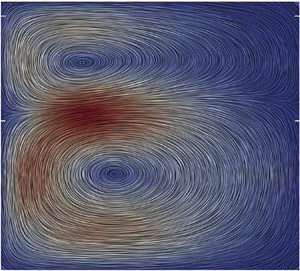
  $(\varGamma , Re) = (5, 150)$; the 2-, 4- and 6-roll states are stacked from the left- to the right-hand side in each panel. It is seen that the density maxima is located near the stationary outer cylinder, but the temperature maxima is located within the annular gap since both cylinders are kept at the same temperature and the added shear work due to the rotation of the inner cylinder is responsible for the increased temperature of the gas. Note that the red blobs in each panel of figure 7(a) correspond to the ‘outward’ jet through which the relatively hotter and rarefied gas (viz. figure 7b) is thrown out from the inner towards the outer cylinder. Comparing the density fields among different roll states in figure 7(b) we find that the density field is relatively more homogeneous in the 6-roll state than in the 2-roll state; the same observation holds for the temperature field too due to the enhanced mixing with increasing number of vortices. The azimuthal velocity fields in figure 7(c), along with the related colourmaps of the specific angular momentum,
 \begin{equation} \mathcal{L}(r,z) =\langle \rho(r,z) v(r,z) r\rangle, \end{equation}
in figure 7(d), further clarify the locations of the outward and inward jets, characterized by higher and lower values, respectively, of both azimuthal velocity and  ${\mathcal {L}}$ for each case. All three states represent stable configurations which have been verified by running long-time simulations for each solution branch at
  $\varGamma =5$.

Figure 7. Colourmaps in the ( $r, z$)-plane of (a) temperature
  $T(r,z)$, (b) density
  $\rho (r,z)$, (c) azimuthal velocity
  $v(r,z)$ and (d) the specific angular momentum
  $\mathcal {L}(r,z) =\langle \rho v r\rangle$; on each panel, 2-roll (left-hand side), 4-roll (middle) and 6-roll (right-hand side) states are shown. The Reynolds number is
  $Re=150$ and the aspect ratio is
  $\varGamma =5$, with other parameters as in figure 6.
With reference to the phase diagram of figure 5, three representative bifurcation diagrams in the ( $u, \varGamma$)-plane are displayed in figures 8(a), 8(b) and 8(c) for Reynolds numbers of
  $Re=75$,
  $120$ and
  $170$, respectively. In each panel, the lower branch with
  $u<0$ corresponds to the ‘normal’ 4-roll state for which there is an inward jet at the midheight of the TC-cell. Note that the 4-roll state represents the primary bifurcation (from the CCF state) at
  $\varGamma =5$, see figure 5. The upper branches in figure 8(a–c) refer to 2-roll (left-hand branch) and 6-roll (right-hand branch) states which are characterized by an outward jet (
 $u>0$) at the midheight of the TC-cell.

Figure 8. Evolution of bifurcation diagrams with Reynolds number in the ( $u, \varGamma$)-plane, where
  $u$ is the radial velocity at the midheight and mid gap: (a)
  $Re=75$, (b)
  $Re=120$ and (c)
  $Re=170$. Note that the dashed lines joining two limit points in panel (b,c) are drawn to guide the eye.
Collectively, the bifurcation diagrams in figures 8(a) ( $Re=75$), 4(c) (
 $Re=100$), 8(b) (
 $Re=120$), 6(c) (
 $Re=150$) and 8(c) (
 $Re=170$) can be stacked together to construct a three-dimensional bifurcation diagram in the (
 $u, Re, \varGamma$)-plane (not shown). The projection of the latter in the (
 $u, Re$)-plane is shown in figure 9(a) for selected values of
  $\varGamma$; while the lower branch of figure 9(a) with
  $u<0$ belongs to the 4-roll state, the upper branches with
  $u>0$ correspond to 2- and 6-roll states. To identify the possible existence of limit points in figure 9(a), additional computations were performed at
  $\varGamma = 5$ by varying
  $Re$ starting with the initial state from both upper and lower branches of figure 9(a). More specifically, starting from the
  $2$-roll branch at
  $Re = 130$ (see the line marked by blue circles in figure 9b), the Reynolds number was decreased in steps of
  ${\rm \Delta} Re = 2$, while starting from the
  $4$-roll branch at
  $Re=110$ (see the line marked by orange diamonds), the Reynolds number was increased in the steps of
  ${\rm \Delta} Re = 2$. The results are summarized in figure 9(b) which confirms discrete jumps between
  $4$- and
  $2$-/
$2$-/ $6$-roll states in the (
 $u, Re$)-plane.

Figure 9. Bifurcation diagrams in ( $u, Re$)-plane for (a) various
  $\varGamma$ and (b)
  $\varGamma =5$. In panel (b), the 2-roll and 4-roll branches have been continued by varying
  $Re$ to verify the existence of any limit point; expectedly, the 2-roll and 6-roll branches are disconnected in the (
 $u, Re$)-plane.
3.3. Role of compressibility on bifurcation structure and patterns
Recall from figure 5 that we found noticeable differences between the compressible ( ${Ma=1}$) and incompressible (
 $Ma=0$, Benjamin (Reference Benjamin1978b); Mullin et al. (Reference Mullin, Pfister and Lorenzen1982); Cliffe (Reference Cliffe1988)) TCF regarding the ‘
 $2\leftrightarrow 4$’ and ‘
 $4\leftrightarrow 6$’-roll transition loci in the (
 $\varGamma , Re$)-plane; the quantitative differences were seen to grow at larger
  $Re$, away from the linear stability threshold. The above results indicate that our nonlinear results differ from the linear stability results of Welsh et al. (Reference Welsh, Kersal'e and Jones2014) who showed that the neutral stability boundary, characterizing the transition between CCF and TVF states, is nearly insensitive to Mach numbers of
  ${Ma}\leq 1$, i.e.
  $Re_{cr}(Ma\leq 1) \approx Re_{cr}(Ma=0)$. On the other hand, they also showed that the critical Reynolds number increases with increasing
  ${Ma}>1$, implying the overall stabilizing role of compressibility on ‘
 $\textrm {CCF}\to \textrm {TVF}$’ transition in axially periodic TCF. In the following, we address the role of compressibility in detail by analysing results over a range of Mach numbers
  $0.2\leq Ma\leq 3$ in the context of axially bounded compressible TCF.
Figure 10(a,b) shows the effects of Mach number on the bifurcation diagram in the ( $u, \varGamma$)-plane; the Reynolds number is set to (a)
  $Re=100$ as in figure 4(c) and 4(b)
  $Re=150$ as in figure 6(b). While the left- and right-hand branches in figure 10(a,b) refer to 2-roll (viz. figure 11c) and 6-roll states, respectively, the middle branch corresponds to a
  $4$-roll state (viz. figure 12c). Comparing three solution branches in figure 10(a), we find that the extent of the subcritical/hysteretic regions increases when the Mach number is decreased to
  $Ma=0.2$, but the transition among different roll states seems to be continuous over
  $\varGamma$ at
  ${Ma=3}$; with increasing
  $Re$, however, the hysteretic transition reappears at
  $Ma=3$, see figure 10(b). A general trend in figure 10(a,b) is a reduction in the magnitude of the midgap, midheight radial velocity,
  $u(r=r_i+\delta /2, z=h/2)$, implying a relatively weaker outward and inward jet (in the bulk) with increasing
  $Ma$.
$Ma$.

Figure 10. Effect of Mach number on the bifurcation diagram in ( $u, \varGamma$)-plane for (a)
  $Re=100$ and (b)
  $Re=150$. Note that the dashed lines joining two limit points are drawn to guide the eye.

Figure 11. Effects of Mach number on the meridional-plane (a) specific angular momentum  ${\mathcal {L}}(r,z)$, (b) temperature
  $T(r,z)$ and (c) streamlines, corresponding to the left-hand upper branch of figure 10(a). On each panel, two snapshots correspond to peripheral Mach number of
  ${Ma} = 0.2$ (left-hand side) and
  $1$ (right-hand side). The Reynolds number is
  $Re=100$ and the aspect ratio is
  $\varGamma =4$.


Referring to different solution branches of figure 10(a) and setting the aspect ratio to  $\varGamma =4$, the meridional plane distributions of (i) specific angular momentum
  ${\mathcal {L}}(r,z)$, (ii) temperature
  $T(r,z)$ and (iii) streamlines are compared in figures 11(a–c) and 12(a–c) for different values of Mach number; while the left- and right-hand snapshots in each panel of figure 11(a–c) correspond to 2-roll states at
  $Ma=0.2$ (left-hand side) and
  $1$ (right-hand side), those in figure 12(a–c) correspond to 4-roll states at
  $Ma=0.2$ (left-hand side),
  $1$ (middle) and
  $3$ (right-hand side). Although the roll structures (panel c) look similar at all
  $Ma$, the temperature fluctuations (panel b) decay, expectedly, for nearly incompressible flows (
 ${Ma}=0.2$) which should vanish at
  ${Ma}=0$. On the other hand, the angular momentum field in figures 11(a) and 12(a) is seen to decay with increasing
  ${Ma}$, implying that the compressibility diminishes angular momentum transport from the inner to the outer cylinder at given
  $Re$.
$Re$.
The right-hand-most snapshots in figure 12(a,c) at  ${Ma}=3$ indicate that the two central vortices are much weaker compared with Ekman vortices (i.e. those located near the end plates). The related evolution of roll structures with increasing aspect ratio can be ascertained from figure 13 which displays streamline patterns at different
  $\varGamma$; this refers to the solution branch marked by triangles in figure 10(a). It is clear that, with increasing
  $\varGamma$, the transition from a 2-roll state (the first panel in figure 13,
  $\varGamma =3.5$, whose origin is tied to Ekman vortices) to a 4-roll state (second, third, fourth and fifth panels at
  $\varGamma =3.7, 4, 5$ and
  $5.5$) is accompanied by the genesis of two daughter modes around the midheight of the annulus, which grow in size with increasing
  $\varGamma$ and subsequently gives birth to a 6-roll state at
  $\varGamma \approx 5.6$. The streamline patterns of two 6-roll states at
  $\varGamma =5.7$ can be ascertained from the two right-hand-most panels in figure 13. The latter two states belong to the hysteresis loop on the solution branch for
  ${Ma}=3$, see figure 10(a) at around
  $\varGamma =5.7$.

Figure 13. Streamline patterns on the meridional-plane for different aspect ratio:  $\varGamma =3.5, 3.7, 4, 5, 5.5, 5.7$ and
  $5.7$ (from left to right); the last two snapshots are for
  $\varGamma =5.7$ that belong to the hysteretic loop for the triangled-curve in figure 10(a). The Mach number is
  $Ma=3$ and the Reynolds number is
  $Re=100$.
Juxtaposing the bifurcation diagrams in figure 10(a,b) at different  ${Ma}$ with those in figure 8 (for
  $Ma=1$), we infer that the increasing Mach number would lead to a shift in the locations of multiroll transitions (
 $2\to 4\to 6$ rolls) and related hysteresis to higher values of Reynolds number. This implies that the overall phase diagram in figure 5 in the (
 $\varGamma , Re$)-plane would be shifted to higher values of
  $Re$ when the Mach number is increased from the incompressible limit. In summary, the primary effects of compressibility (
 $Ma\uparrow$) on symmetric roll states are: (i) a delayed onset of multiroll transitions to larger
  $Re$; (ii) measurable changes in the successive higher-order (‘
 $2 \leftrightarrow 4$’ and ‘
 $4 \leftrightarrow 6$’-roll) transition loci in the (
 $\varGamma , Re$)-plane (viz. figure 5) in comparison to what is known in incompressible TCF (Benjamin Reference Benjamin1978b; Mullin et al. Reference Mullin, Pfister and Lorenzen1982; Cliffe Reference Cliffe1988); (iii) the emergence of weaker outward jets (figure 10a,b and 12a,c); and (iv) relatively larger (and hence stronger) Ekman vortices (viz. figure 12c) near the two end walls. Collectively, the weakening of outward jets and the strengthening of Ekman vortices with increasing
  $Ma$ (for given
  $Re$) are responsible for the decreased angular momentum transport (figure 12a), from the rotating inner cylinder to the outer cylinder in the same limit, and consequently to the overall stabilizing role of compressibility on nonlinear Taylor vortices.
4. Asymmetric vortices at $\varGamma =O(1)$: anomalous (single-roll) modes

Experiments carried out on incompressible TCF by Benjamin & Mullin (Reference Benjamin and Mullin1981) confirmed that the asymmetric 2-roll states (i.e. the single-roll, or, anomalous modes), a smaller vortex coexisting with a larger one, can appear when the aspect ratio of the TC-cell is of order one, i.e.  $\varGamma =h/\delta =O(1)$; this was verified first in direct numerical simulations of Navier–Stokes equations by Cliffe (Reference Cliffe1983). The phase diagram of such asymmetric 2-roll modes was subsequently extended in the numerical and experimental work of Pfister et al. (Reference Pfister, Schmidt, Cliffe and Mullin1988). A computational methodology to uncover the compressible analogues of such asymmetric 2-roll states is outlined in § 4.1, followed by (i) a description of its complete phase diagram in the (
 $\varGamma , Re$)-plane § 4.2, (ii) the characterization of bifurcation scenario and patterns and (iii) the role of compressibility in § 4.3.
4.1. Tracking asymmetric 2-roll modes via a homotopy method
An example of an asymmetric 2-roll state, with a smaller vortex lying over a larger one, is shown in figure 14(b–d) which was obtained using the following procedure. The simulation is started with an axial temperature gradient which is switched on at  $t=0$ by setting the top and bottom wall temperatures to
 \begin{equation} T(z=h) = 1 + \epsilon \quad \mbox{and} \quad T(z=0)=1- \epsilon,\end{equation}
respectively; this initial condition breaks the midplane symmetry of the temperature field, see figure 14(e). The time evolution of this initial condition, with a value of  $\epsilon =-0.1$, yields an asymmetric 2-roll state as confirmed by figure 14(b,f), at time
  $t=8$; this asymmetric state (with asymmetric end-wall conditions (4.1a,b)) remained stable with time, which was verified by continuing simulations down to
  $t=16$ (not shown); other parameters are
  $\varGamma =1$,
  $Ma=1$ and
  $Re=190$. After reaching the steady state the temperature gradient is switched off by setting
  $\epsilon =0$ at
  $t=16$, and the simulation is further continued in time. Figures 14(c,g) confirm that this asymmetric 2-roll state is indeed stable with ‘symmetric’ temperature boundary conditions (
 $\epsilon =0$) at two axial ends. Note that the location of the larger/smaller vortex depends on the sign of the homotopy parameter
  $\epsilon$ in (4.1a,b); for example, starting the same simulations with
  $\epsilon =0.1$ yielded figure 14(d,h) with the larger vortex being on the top of the smaller one, i.e. a reflection of the mode shown in figure 14(c,g) about its midheight.

Figure 14. Stable asymmetric 2-roll state obtained with asymmetric temperature boundary condition (4.1a,b): meridional velocity field (panels a–d) and temperature contours (panels e–h). (a,e) Axial temperature gradient ( $\epsilon =-0.1$) switched on at
  $t=0$; (b,f) asymmetric mode settles at
  $t = 8$ which is continued up to
  $t=16$ (not shown) at which the temperature gradient is switched off (
 $\epsilon =0$); (c,g) final state
  $t=80$ (with
  $\epsilon =0$) which survives at larger times. (d,h) Starting with
  $\epsilon =0.1$ leads to a ‘mirror-image’ asymmetric 2-roll state with the larger vortex lying on top of the smaller one. Parameter values are
  $Re=190$,
  $Ma=1$ and
  $\varGamma =1$.
In the context of compressible TCF, the asymmetric temperature protocol (4.1a,b) can be used as a computationally inexpensive alternative to Schaeffer's homotopy method (Schaeffer Reference Schaeffer1980) to track anomalous modes. It should be noted that the mathematical framework of Schaeffer (Reference Schaeffer1980) was numerically implemented by Cliffe (Reference Cliffe1983, Reference Cliffe1988) and others to track both normal and anomalous solution branches that helped in seamlessly tying the ‘periodic’ and ‘axially bounded’ models of incompressible TCF. The latter technique uses mixed Dirichlet–Neumann axial boundary conditions on the velocity field,
 \begin{equation} (1-\epsilon) \frac{\partial (u,v)}{\partial z} \pm \epsilon (u,v) = 0 \quad \mbox{and} \quad w=0 \quad \mbox{at}\ z=0, h, \end{equation}
that interpolates between no-slip and periodic/free-slip end walls via a homotopy parameter  $\epsilon \in (0,1)$. The grid refinement needed to accurately discretize velocity derivatives at the end walls is likely to increase the computational cost of the Schaeffer (Reference Schaeffer1980) method in comparison to the present method (4.1a,b). While (4.2a,b) has been extensively used to track both symmetric and asymmetric anomalous modes, the non-isothermal and compressible nature of the gas offer two alternative axial boundary conditions (
 $T=1\pm \epsilon$, or,
  $\rho =1\pm \epsilon$ at
  $z=0$ and
  $h$) to track ‘asymmetric’ modes in compressible TCF as demonstrated in this work. It should be noted that the ‘symmetric’ anomalous modes can, in principle, be constructed via the present technique by stacking an even number of asymmetric solutions via an appropriate mapping of related control parameters – the related issues are left for a future work.
Returning to the TCF with symmetric axial boundary conditions, an example of ‘ $1\to 2$’-roll transition with decreasing
  $Re$ is shown in figure 15(a–c), with the aspect ratio being set to
  $\varGamma =1.2$. The asymmetric 2-roll state at
  $Re=240$ (figure 15a) was realized by running the simulation using (4.1a,b) as the initial condition as described in the preceding paragraph. The resulting equilibrium solution (with
  $\epsilon =0$) at
  $Re=240$ was continued subsequently by decreasing
  $Re$, in steps of
  ${\rm \Delta} Re=2$, up to
  $Re=180$. The corresponding bifurcation diagram in the (
 $|w|, Re$)-plane, shown in figure 15(d), confirms the discontinuous nature of ‘
 $1\to 2$’-roll transition at
  $\varGamma =1.2$; while the inverted triangles denote the above downsweep data, the up triangles represent an ‘upsweep’ run starting from
  $Re=180$ (figure 15c) up to
  $Re=240$ which tracked the symmetric 2-roll (
 $|w|=0$) branch. From a comparison between figures 15(a) and 15(b) we find that the location of the outward jet is shifted up with increasing
  $Re$, implying an increased size of the larger vortex, and the smaller vortex is further squeezed towards the top left-hand corner. In comparison to the bifurcation diagram in figure 15(d) for
  $\varGamma =1.2$, the bifurcation becomes subcritical when the aspect ratio of the TC-cell is decreased to
  $\varGamma =0.9$, see figure 15(e); the related details are discussed in appendix B (supplementary materials). The nature of bifurcation over a range of
  $\varGamma$, and the phase diagram of symmetric and asymmetric 2-roll states, are analysed below.

Figure 15. Transition from ‘asymmetric’ to ‘symmetric’ 2-roll states with decreasing Reynolds number: velocity vectors in the ( $r,z$)-plane at (a)
  $Re=240$, (b)
  $Re=200$ and (c)
  $Re=180$; the aspect ratio is
  $\varGamma =1.2$ and
  $Ma=1$. (d,e) Bifurcation diagrams in the (
 $|w|, Re$)-plane at (d)
  $\varGamma =1.2$ and (e)
  $\varGamma =0.9$, where
  $w\equiv w(r=r_i+\delta /2,z=h/2)$ is the midgap, midheight axial velocity and the ramp rate is
  $\textrm {d} Re/\textrm {d} t=2\times 10^{-2}$; the dashed line (postulated) in each panel denotes unstable states.
4.2. Phase diagram and its comparison with incompressible limit
Figure 16(a) displays the phase diagram in the ( $\varGamma , Re$)-plane, depicting the transition between symmetric and asymmetric 2-roll (i.e. the single-roll mode) states; the ‘open’ symbols were obtained by following the ‘
 $\varGamma$ increase/decrease’ protocol (see figure 17). The black lines, representing approximate phase boundaries between ‘
 $1\leftrightarrow 2$’-roll transitions, are drawn to guide the eye; other parameters are
  $Ma=1$ and
  $Pr=1$. Note that the tracking of the midplane asymmetric modes was time consuming since the ramp rate (
 $\textrm {d}\varGamma /\textrm {d} t$) had to be extremely small; for example,
  $\textrm {d}\varGamma /\textrm {d} t$ was an order of magnitude smaller than that used to track transitions among symmetric rolls in figure 5.

Figure 16. (a) Phase diagram in the ( $\varGamma , Re$)-plane, obtained from the ‘
 $\varGamma$ increase/decrease’ protocol, for
  $\eta =1/2$,
  ${Ma}=1$ and
  ${Pr=1}$; the ramp rate is
  ${\textrm {d}\varGamma }/{\textrm {d} t} = 2.5\times 10^{-4}$ (with an increment of
  $\textrm {d}\varGamma =0.01$ after every
  $4\times 10^{6}$ time steps). While the ‘open’ squares and up triangles were extracted from the upsweep run in
  $\varGamma$, the diamonds and down triangles were extracted from the downsweep run in
  $\varGamma$; the ‘filled’ squares and circles (at
  $\varGamma =0.9, 0.95, 1.0, 1.05, 1.1, 1.15$ and
  $1.2$) were obtained from the ‘
 $Re$ increase/decrease’ protocol described in § 4.1 (see appendix B in the supplementary materials). The lines, postulated phase boundaries, are drawn to guide the eye; the yellow shaded region represents the coexistence of asymmetric and symmetric 2-roll states. (b) Phase diagram for incompressible TCF in the (
 $\varGamma , Re$)-plane, adapted from Pfister et al. (Reference Pfister, Schmidt, Cliffe and Mullin1988), that holds for a radius ratio of
  $\eta =1/2$. The blue shaded region, over
  $\varGamma ^{sub}_c \leq \varGamma \leq \varGamma _c^{LP}$, represents subcritical bifurcations with varying
  $Re$ (say, in the (
 $u, Re$)-plane); the green-shaded region at
  $\varGamma >\varGamma _c^{LP}$ represent disconnected single-roll solutions coexisting with symmetric 2-roll solutions, with the loci of limit points being marked by the black circled-dashed line.

Figure 17. Effect of Mach number on bifurcation diagrams in the ( $|w|, \varGamma$)-plane, where
  $w$ is the midheight, midgap axial velocity: (a)
  $Re=180$, (b)
  $Re=200$, (c)
  $Re=220$ and (d)
  $Re=240$. The aspect ratio
  $\varGamma$ was changed in steps of
  ${\rm \Delta} \varGamma =0.01$ after every
  $4\times 10^6$ time steps, resulting in a ramp rate of
  $\textrm {d}\varGamma /\textrm {d} t=2.5\times 10^{-4}$ and the grid size is
  $21\times 21$. Panel (e) is a zoomed version of panel (c) for
  $Ma=3$ using two ramp rates of
  $\textrm {d}\varGamma /\textrm {d} t=2.5\times 10^{-4}$ (green triangles) and
  $2.5\times 10^{-3}$ (black triangles). The curly red arrow in panel (e) indicates the continuous nature of the solution branch during the ‘upsweep’ run; see the text for details.
To check the robustness of figure 16(a), the ‘ $Re$ increase/decrease’ protocol of § 4.1 was employed to identify the limit point and bifurcation points for ‘
 $1\leftrightarrow 2$’-roll transition at selected values of
  $\varGamma =0.9, 0.95, 1.0, 1.05, 1.1, 1.15$ and
  $1.2$, refer to figure 15(d) and 15(e) for the bifurcation diagrams in the (
 $|w|, Re$)-plane at
  $\varGamma =1.2$ and
  $0.9$, respectively. These additional data are marked by the ‘filled’ squares (bifurcation point) and circles (limit point) in figure 16(a). It is seen that both sets of data agree closely with each other, confirming the robustness of the phase diagram in figure 16(a), including the yellow shaded region that corresponds to the coexistence of (i) symmetric and (ii) asymmetric 2-roll states. While the white region bounded by the yellow-shaded region in figure 16(a) refers to ‘stable’ asymmetric 2-roll states, the symmetric 2-roll states exist on the exterior of the limit point branch. Comparing figure 16(a) with the phase diagram for the ‘higher-order’ symmetric rolls in figure 5, we find that the asymmetric 2-roll states appear at much larger values of the Reynolds number
  $Re$ for specified
  $Ma$.
$Ma$.
Figure 16(a) should be contrasted with figure 16(b) that represents the phase diagram of ‘ $1\leftrightarrow 2$’-roll transition for incompressible TCF which has been adapted from the experimental and numerical study of Pfister et al. (Reference Pfister, Schmidt, Cliffe and Mullin1988). The left-hand branch of figure 16(b) represents supercritical bifurcation, whereas a part of the right-hand branch (the blue dotted line over
  $\varGamma _c^{sub}\leq \varGamma \leq \varGamma _c^{LP}$) represents subcritical bifurcations; the green-shaded region at
  $\varGamma \geq \varGamma _c^{LP}$ represents disconnected single-roll solutions that coexist with stable symmetric 2-roll solutions at any
  $Re$ above the limit point branch marked by the circled dashed line. Therefore, in contrast to the incompressible TCF (figure 16b), the ‘
 $1\leftrightarrow 2$’-roll transition in compressible TCF (viz. figure 16a at
  $Ma=1$) is subcritical/hysteretic at any aspect ratio
  $\varGamma$ of the TC-cell. The above general finding holds also at higher values of
  $Ma>1$ as we demonstrate below, via an analysis of the underlying bifurcation diagrams and the hydrodynamic fields.
4.3. Hysteretic transition and the role of compressibility
The subcritical/hysteretic bifurcations uncovered in figure 16(a) are further confirmed from the bifurcation diagrams in figure 17(a–d) which display the variations of the midheight, midgap axial velocity,
 \begin{equation} w \equiv w\left(r=r_i+\frac{\delta}{2}, z=\frac{h}{2} \right),\end{equation}
as a function of  $\varGamma$ for (a)
  $Re=180$, (b)
  $Re=200$, (c)
  $Re=220$ and (d)
  $Re=240$; while the blue circles denote the data for
  $Ma=1$, the green triangles represent
  $Ma=3$. Note that the axial velocity at the midheight and midgap vanishes (i.e.
  $w=0$) for symmetric rolls and
  $|w|>0$ for asymmetric rolls. The red arrows in each panel of figure 17 indicate abrupt jumps from the 2-roll state to the asymmetric 2-roll state and vice versa during upsweep (increasing
  $\varGamma$) and downsweep (decreasing
  $\varGamma$) protocols. Juxtaposing the bifurcation diagrams for
  $Ma=1$ in figure 17(a–d) with the phase diagram in figure 16(a), we find that the outer phase boundary in figure 16(a) represents the loci of limit points, while its inner boundary refers to the loci of (subcritical) bifurcation points.
Comparing the bifurcation diagrams between  $Ma=1$ and
  $Ma=3$ in each panel of figure 17(a–d), we find that the single-roll mode persists at
  $Re=180$ and
  $200$ for
  $Ma=1$ but are absent at
  $Ma=3$; the single-roll solution starts appearing at
  $Ma=3$ when the Reynolds number is increased to
  $Re\geq 220$ (panel c). This suggests that the phase diagram of ‘
 $1\leftrightarrow 2$’-roll transitions in the (
 $\varGamma , Re$)-plane, such as in figure 16(a), would shift to larger values of
  $Re$ with increasing Mach number.
Returning to figure 17, we confirmed that the left- and right-hand hysteresis loops are robust features of axially bounded TCF since both loops remained intact with changing ramp rate  $\textrm {d}\varGamma /\textrm {d} t$ (see appendices B and C in the supplementary material for details). A further confirmation in this regard can be ascertained from figure 17(e) that shows the near invariance of the shape of the bifurcation diagram at
  $Ma=3$ with two ramp rates
  $d\varGamma /dt=2.5\times 10^{-4}$ (green triangles) and
  $2.5\times 10^{-3}$ (black triangles) that differ by an order of magnitude. Recall from figure 16(b) that the left-hand hysteresis loop of figure 17 is completely absent in the incompressible limit (figure 16b,
  $Ma=0$) and therefore its existence at
  $Ma>0$ is solely due to the compressibility of the gas. The unequivocal support for the latter observation is ascertained from figure 17(c,d) that compares the bifurcation diagrams for
  $Ma=1$ and
  $3$; ‘the range of
  $\varGamma$ spanning the left-hand hysteresis loop increases with increasing
  $Ma$ at given
  $Re$’. Moreover, our data at
  $Ma=0.2$ (not shown) indicate a decreased size of the left-hand hysteresis loop, thus confirming its disappearance in the incompressible limit
  $Ma\to 0$. From the above discussion, we conclude that the ‘
 $1\leftrightarrow 2$’-roll transition in compressible TCF is hysteretic at any
  $\varGamma$ (figure 16a) in contrast to the super-critical/subcritical nature of bifurcation at smaller/larger values of
  $\varGamma$, respectively, in its incompressible counterpart (figure 16b).
An interesting feature of the bifurcation diagram in figure 17(e) is that the order parameter (4.3) is close to zero at  $\varGamma \sim 1.07$, resulting in an apparent kink/discontinuity in the (
 $|w|, \varGamma$)-plane – this occurs within the range of
  $\varGamma$ over which the single-roll solution should be a stable state. The reason for the appearance of this kink in the (
 $|w|, \varGamma$)-plane can be explained as follows: the topological changes in the velocity patterns with increasing
  $\varGamma$, see figure 18(a–c), may render the midgap, midheight location, at which the order parameter is measured, to coincide with the centre of the larger vortex, resulting in
  $w(r_i+\delta /2, h/2)\approx 0$ at some value of
  $\varGamma$. The corresponding pattern still represents an ‘asymmetric’ state (not a symmetric 2-roll for which
  $w=0$ as well) as confirmed in figure 18(b). The continuous nature of the solution branch can be better appreciated if we replot the bifurcation diagrams, such as those in figure 17(c,d), in the (
 $w, \varGamma$)-plane.

Figure 18. Meridional velocity field at  $Re = 220$ and
  $Ma=3$: (a)
  $\varGamma =0.93$, (b)
  $1.07$ and (c)
  $1.17$; the red circle in each panel denotes the midgap, midheight location. Refer to figure 17(e) for the corresponding bifurcation diagram in the (
 $|w|, Re$)-plane.
Lastly, to establish the connection of the asymmetric 2-roll mode found in the present study to those in incompressible TCF (Benjamin & Mullin Reference Benjamin and Mullin1981; Cliffe Reference Cliffe1983; Pfister et al. Reference Pfister, Schmidt, Cliffe and Mullin1988), we numerically continued the steady solution found at  $Ma = 1$ (see figure 14 that holds for
  $Re = 190$,
  $\varGamma = 1$ and
  $Pr = 1$) to
  $Ma = 0.1$ in steps of
  ${\rm \Delta} Ma = 0.1$. A sample calculation is summarized in figure 19 which displays the meridional velocity field (a–c), the temperature (d–f) and the specific angular momentum (g–i), with other parameters as in figure 14. The asymmetric mode manifested using (4.1a,b) was allowed to settle at
  $Ma = 1$, see the left-hand column of figure 19; after reaching the steady state,
  $Ma$ was lowered to
  $Ma = 0.9$ and the flow was allowed to stabilize again. The grid size is
  $21 \times 21$ and the requirement on time-step (
 ${\rm \Delta} t$) was severe towards the incompressible limit; for example, a time step of
  ${\rm \Delta} t = 10^{-5}$ is used for
  $Ma\geq 0.7$ and
  ${\rm \Delta} t=10^{-7}$ for smaller
  $Ma$ to obtain converged solutions. The above procedure was checked for both positive and negative values of
  $\epsilon$, and, in both cases, the asymmetric 2-roll modes survived until
  $Ma = 0.1$. We conclude that the single-roll modes uncovered in the present study are indeed connected to those found in its incompressible counterpart.

Figure 19. Asymmetric 2-roll (i.e. ‘single-roll’) modes at  $Ma = 1$ (a,d,g),
  $Ma = 0.5$ (b,e,h) and
  $Ma = 0.1$ (c,f,i); meridional velocity vectors (a–c), temperature contours (d–f) and angular momentum contours (g–i). Parameter values are
  $Re = 190$,
  $Pr=1$ and
  $\varGamma = 1$.
It is clear from the middle row of figure 19 that the magnitudes of temperature fluctuations decrease and approach zero as we move towards the incompressible limit ( $Ma\to 0$). The bottom row of figure 19 confirms that the angular momentum transport via asymmetric 2-roll mode is enhanced in the incompressible limit – this finding is similar to that for higher-order symmetric rolls (viz. figures 10–12) as summarized in the last paragraph of § 3.3. Collectively, therefore, the compressibility aids in stabilizing both asymmetric and symmetric Taylor vortices and the underlying multiroll transitions.
5. Summary and conclusion
This is the first study to analyse the effects of (i) the gas compressibility and (ii) the finite aspect ratio ( $\varGamma =h/\delta$) on the onset of nonlinear Taylor vortices and the related bifurcation scenario, resulting in the multiplicity of states, in ‘axially bounded’ TCF. An in-house-developed finite-difference code has been used to solve the axisymmetric Navier–Stokes–Fourier equations for an ideal (monatomic) gas. Focussing on the case of the inner cylinder rotating with stationary end plates in the wide-gap limit (a radius ratio of
  $\eta =R_i/R_o=1/2$), the aspect ratio
  $\varGamma$ was changed by changing the length of the cylinders. The role of compressibility was analysed by varying the Mach number (
 $Ma$) ranging from the incompressible limit (
 $Ma\to 0$) to
  $Ma=3$.
The transitions between midplane symmetric  $2k$ and
  $2(k+1)$ rolls and the associated hysteresis were studied by increasing/decreasing
  $\varGamma$ over a range of inner-cylinder Reynolds number (
 $Re$) for specified values of
  $Ma$ in § 3. The ‘
 $2k\rightarrow 2(k+1)$’-roll transition was found to be hysteretic, resulting in the coexistence of different number of ‘normal’ Taylor vortices (such as
  $2+4$-,
  $4+6$- and
  $2+4+6$-rolls) over the ranges of (i) aspect ratio
  $\varGamma \in (2,7)$ and (ii) inner-cylinder Reynolds number
  $Re \leq 200$. The phase diagram of patterns was constructed in the (
 $\varGamma , Re$)-plane that delineates the loci of bifurcation points and limit points, identifying the coexisting regions of different-numbered vortices in the (
 $\varGamma , Re$)-plane. A comparison of our phase diagram (viz. figure 5) with the experimental (Benjamin Reference Benjamin1978b; Mullin et al. Reference Mullin, Pfister and Lorenzen1982) and numerical (Cliffe Reference Cliffe1988) data on incompressible TCF indicated that although the locations of cusps agree well with those of their incompressible (
 $Ma=0$) counterpart, there are significant differences between
  $Ma=0$ and
  $Ma=1$ about the loci of both ‘
 $2\leftrightarrow 4$’ and ‘
 $4\leftrightarrow 6$’-roll transitions in the (
 $\varGamma , Re$)-plane. In addition, the comparison between
  $Ma=1$ and
  $Ma=3$ on the bifurcation diagrams in the (
 $u, \varGamma$)-plane (viz. figure 10) and on the meridional-plane hydrodynamic fields (viz. figure 12) confirmed that (i) the even-roll transitions and the related hysteresis occur at larger values of
  $Re$, (ii) the outward jets become weaker and (iii) the Ekman vortices become stronger as the Mach number is increased, implying the overall stabilizing role of compressibility on nonlinear Taylor vortices.
For small aspect ratio TC-cells, the ‘asymmetric’ 2-roll modes (i.e. single-roll or ‘anomalous’ modes, Benjamin & Mullin (Reference Benjamin and Mullin1981)) were realized in § 4. An analogue of the Schaeffer (Reference Schaeffer1980) homotopy method was implemented by imposing an asymmetric temperature protocol (4.1a,b) between top and bottom end walls. The phase diagram of patterns, consisting of symmetric and asymmetric 2-roll states, was constructed in the ( $\varGamma , Re$)-plane. It was shown that the asymmetric 2-roll modes appear at much larger values of
  $Re$, compared with that for symmetric higher-order rolls at any
  $Ma$. Contrasting the phase diagram of ‘
 $1\leftrightarrow 2$’-roll transition in compressible TCF with that of its incompressible counterpart (viz. figure 16), we found that the left-hand branch of the phase boundary (i.e. at smaller aspect ratios,
  $\varGamma <1$) in the (
 $\varGamma , {\mathrm Re}$)-plane is subcritical in a compressible gas compared with the supercritical nature of bifurcation in its incompressible counterpart. In particular, the size of the left-hand hysteresis loop (viz. figure 17c,d) was found to increase with increasing
  $Ma$ at specified values of
  $Re$; in other words, the range of
  $\varGamma <1$ over which the single- and 2-roll modes coexist becomes larger with increasing compressibility. Therefore, the gas compressibility is responsible for the genesis of the left-hand hysteresis loop at
  $\varGamma <1$ in figure 16(a) which is a novel feature of compressible TCF.
For both symmetric and asymmetric modes, it was shown that increasing  $Ma$ results in a relatively weaker angular momentum field in the meridional plane (viz. figures 12a and 19g–i), indicating a lesser amount of angular momentum being transported from the rotating inner cylinder to the outer cylinder in the same limit. The latter finding is a direct consequence of (i) the weakening of the outward jets and (ii) the strengthening of the Ekman vortices, as discussed in § 3.3 for higher-order symmetric modes. Our general finding that the critical Reynolds number increased with increasing
  $Ma$ (and hence the stabilizing role of compressibility) agrees qualitatively with the experimental results of Kuhlthau (Reference Kuhlthau1960), thus extending the predictions of the linear stability analyses (Manela & Frankel Reference Manela and Frankel2007; Welsh et al. Reference Welsh, Kersal'e and Jones2014) to the nonlinear regime.
We have not tracked the anomalous ‘symmetric’ modes at  $\varGamma \geq 2$, and the role of compressibility on these modes can be analysed to ascertain the complete bifurcation picture in axially bounded compressible TCF. Also, a quantitative analysis of the effect of compressibility on the angular-momentum transport and hence on the torque scaling, considering higher-Reynolds-number regime, can be taken up in a future work. This is likely to uncover the compressible analogue of oscillatory modes (Lorenzen et al. Reference Lorenzen, Pfister and Mullin1982; Jones Reference Jones1985) that are known to exist in axially bounded incompressible TCF at
  $Re=O(500)$. The latter would require three-dimensional simulations allowing azimuthal variations. The work in this direction is in progress.
Acknowledgements
P.A. would like to sincerely thank Mr T. Dhar for help in arranging remote access to computers@GrainLab to run the codes during 2019–2020. We also thank Mr Dhar for drawing a preliminary version of the sketch in figure 16(b).
Declaration of interests
The authors report no conflict of interest.
Supplementary material
Supplementary material is available at https://doi.org/10.1017/jfm.2020.897.


