


INTRODUCTION
Phytoplankton account for approximately 50% of global primary production on Earth (Falkowski & Raven, Reference Falkowski and Raven2007) and constitute nearly all of marine primary productivity (Mackas, Reference Mackas2011). They contribute to modulating the total CO2 concentration and pH of the ocean, which, together with physical processes (e.g. solar energy input, sea–air heat exchanges, upwelling of subsurface waters and mixed layer thickness), dictates air–sea CO2 gas exchange (Takahashi et al., Reference Takahashi, Sutherland, Sweeney, Poisson, Metzl, Tilbrook, Bates, Wanninkhof, Feely, Sabine, Olafsson and Nojiri2002). Thus, phytoplankton play a crucial role in the global carbon cycle (Brewin et al., Reference Brewin, Sathyendranath, Hirata, Lavender, Barciela and Hardman-Mountford2010); consequently, any widespread drop in phytoplankton biomass would almost certainly have severe ecological consequences (Mackas, Reference Mackas2011). Due to the important global role of phytoplankton, monitoring biomass and estimation of the composition has a major importance for understanding the structure and dynamics of pelagic ecosystems (Jeffrey & Vesk, Reference Jeffrey, Vesk, Jeffrey, Mantoura and Wright1997; Ediger et al., Reference Ediger, Soydemir and Kideys2006; Nair et al., Reference Nair, Sathyendranath, Platt, Morales, Stuart, Forge, Devred and Bouman2008).
Classically, phytoplankton are studied by microscopy involving identification, counting of cells, measuring their cell size and converting volumes to carbon biomass (Utermöhl, Reference Utermöhl1958; Booth, Reference Booth, Kemp, Sherr and Cole1993; Eker-Develi et al., Reference Eker-Develi, Berthon and Linde2008). As a technique, it requires extensive time for sample preparation, counting and personal skills. Furthermore, smaller phytoplankton (e.g. picoplankton) can be difficult to identify, since they lack taxonomically useful external morphological features; yet, they are now recognized as being significant contributors to the primary productivity (Mackey et al., Reference Mackey, Mackey, Higgins and Wright1996). In addition, many species are very fragile and do not survive sample fixation (Gieskes & Kraay, Reference Gieskes and Kraay1983). However, high performance liquid chromatography (HPLC) methods have been developed in more recent years giving accurate chlorophyll-a (Chl-a) and other marker pigment concentrations providing an estimate of biomass and information on the composition of the phytoplankton community (Mantoura & Llewellyn, Reference Mantoura and Llewellyn1983). The introduction of HPLC pigment analysis facilitated easy and fast separation, identification and quantification of phytoplankton pigments. A large number of samples can be processed by HPLC allowing a more thorough examination of the structure and dynamics of phytoplankton populations compared to microscopy (Schlüter et al., Reference Schlüter, Mohlenberg, Havskum and Larsen2000). Furthermore using HPLC pigment data the quantitative composition of complex phytoplankton populations can be determined by means of pigment ratios (Higgins et al., Reference Higgins, Wright, Schlüter, Roy, Llewellyn, Egeland and Johnson2011). One of the methods used to do this is CHEMTAX.
CHEMTAX (Mackey et al., Reference Mackey, Mackey, Higgins and Wright1996) is a program (v.1.95, Microsoft Excel-based) that uses factor analysis and a steepest descent algorithm to determine the best fit to the data with a given input matrix of pigment ratios. Using an iterative process for a given input matrix, the software optimizes the pigment ratios for each group and applies the final ratio to the total Chl-a in each sample to determine the proportion of Chl-a concentration attributed to each phytoplankton group in the community. CHEMTAX has been widely used to characterize phytoplankton composition in different regions of the world oceans (Mackey et al., Reference Mackey, Mackey, Higgins and Wright1996; Schlüter et al., Reference Schlüter, Mohlenberg, Havskum and Larsen2000; Havskum et al., Reference Havskum, Schlüter, Scharek, Berdalet and Jacquet2004; Llewellyn et al., Reference Llewellyn, Fishwick and Blackford2005; Eker-Develi et al., Reference Eker-Develi, Berthon and Linde2008; Kozlowski et al., Reference Kozlowski, Deutschman, Garibotti, Trees and Vernet2011). However, the application of the CHEMTAX program to coastal and estuary regions, is limited by the lack of known pigment ratios (Wright et al., Reference Wright, Thomas, Marchant, Higgins, Mackey and Mackey1996; Eker-Develi et al., Reference Eker-Develi, Berthon, Canuti, Slabakova, Moncheva, Shtereva and Dzhurova2012).
The Black Sea is a unique marine environment that represents one of the largest inland basins in the world (Yilmaz et al., Reference Yilmaz, Tugrul, Polat, Ediger, Coban and Morkoc1998; Yunev et al., Reference Yunev, Vladimir, Basturk, Yilmaz, Kideys, Moncheva and Konovalov2002), as such it receives a considerable amount of chemicals, organic matter and nutrients from surrounded rivers (especially in the western Black Sea via the River Danube) (Eker-Develi & Kideys, Reference Eker-Develi and Kideys2003; Yilmaz et al., Reference Yilmaz, Coban-Yildiz and Tugrul2006). The Black Sea is also characterized by two large strong cyclonic gyres in its eastern and western parts embedded in a basin-wide cyclonic boundary (rim) current (Oguz et al., Reference Oguz, Latun, Latif, Vladimirov, Sur, Markov, Ozsoy, Kotovshchikov, Eremeev and Unluata1993); these affect the overall productivity of the basin. The salinity never exceeds 17 psu, and excess precipitation together with run-off from the Rivers Danube, Dniester, and Don creates a surface low salinity layer overlying a halocline at about 100 m (Longhurst, Reference Longhurst2007). The presence of the permanent and strong halocline interface inhibits vertical mixing. Moreover, the density gradient is the major reason for the anoxic and sulphidic condition of the sub-halocline waters (Ozsoy & Unluata, Reference Ozsoy and Unluata1997).
Phytoplankton in terms of abundance, biomass and species composition, have been measured in the Black Sea over many decades (Eker et al., Reference Eker, Georgieva, Senichkina and Kideys1999). The ecosystem of the Black Sea showed large shifts during the 1970s and 1980s due to intense eutrophication (Mee, Reference Mee1992; Kideys, Reference Kideys1994; Zaitsev & Alexandrov, Reference Zaitsev, Alexandrov, Ozsoy and Mikaelyan1997). During this time, phytoplankton responded to qualitative and quantitative changes in community composition; for example, intensified blooms and changes in class structure, with a pronounced dominance of dinoflagellates compared to diatoms (Kideys, Reference Kideys1994). In more recent years, there have been some signs of recovery, with a reduction in nutrient loading (McQuatters-Gollop et al., Reference McQuatters-Gollop, Mee, Raitsos and Shapiro2008). Until the 1980s the seasonal phytoplankton dynamics in the Black Sea consisted of a strong diatom and dinoflagellate-dominated spring bloom, followed by a secondary bloom of mainly coccolithophores appearing in the autumn in both the coastal and open waters (Sorokin, Reference Sorokin and Ketchum1983; Vedernikov & Demidov, Reference Vedernikov and Demidov1993). Recently, additional summer blooms of dinoflagellates and coccolithophorids (mainly Emiliania huxleyi Hay & Mohler) have been more frequently reported (Hay et al., Reference Hay, Honjo, Kempe, Itekkot, Degens, Konuk and Izdar1990; Sur et al., Reference Sur, Ozsoy, Ilyin and Unluata1996; Yilmaz et al., Reference Yilmaz, Tugrul, Polat, Ediger, Coban and Morkoc1998; Yayla et al., Reference Yayla, Yilmaz and Morkoc2001). Overall, the Black Sea contains a wide diversity, with 750 identified species, including freshwater and estuarine species, with diatoms reported as the dominant group (46% of total phytoplankton biomass) and dinoflagellates as the next important group (27%) (Zaitsev & Mamaev, Reference Zaitsev and Mamaev1997).
Phytoplankton studies in the Black Sea have mainly focused on the northern shelves (Ivanov, Reference Ivanov1965; Bologa, Reference Bologa1986; Bodeanu, Reference Bodeanu1989, Reference Bodeanu, Smayda and Shimizu1993; Cociasu et al., Reference Cociasu, Diaconu, Popa, Buga, Nae, Dorogan, Malciu, Ozsoy and Mikaelyan1997; Moncheva & Krastev, Reference Moncheva, Krastev, Ozsoy and Mikhaelian1997; Zaitsev & Alexandrov, Reference Zaitsev, Alexandrov, Ozsoy and Mikaelyan1997; Moncheva et al., Reference Moncheva, Gotsis-Skretas, Pagou and Krastev2001) rather than the southern Black Sea (Karacam & Duzgunes, Reference Karacam and Duzgunes1990; Feyzioglu, Reference Feyzioglu1994; Uysal & Sur., Reference Uysal and Sur1995; Eker et al., Reference Eker, Georgieva, Senichkina and Kideys1999; Eker-Develi & Kideys, 2003; Feyzioglu & Seyhan, Reference Feyzioglu and Seyhan2007). In addition, these are primarily based on microscopy examination. Consequently, whilst there have been many efforts to document phytoplankton dynamics in the Black Sea, there have been few studies that have used the more comprehensive profiling using HPLC (Ediger et al., Reference Ediger, Soydemir and Kideys2006; Eker-Develi et al., Reference Eker-Develi, Berthon, Canuti, Slabakova, Moncheva, Shtereva and Dzhurova2012). Therefore, our principal aim was to investigate phytoplankton community structure and dynamics in the southern Black Sea continental shelf area using HPLC pigments-CHEMTAX analysis, microscopy cell counts and carbon biomass estimates of phytoplankton for each taxonomic class. We have compared an offshore station with a shallower inshore station in the south-eastern Black Sea and examined spatio-temporal trends vertically at monthly intervals during 2009.
MATERIALS AND METHODS
Study area and sampling strategy
Samples were collected monthly from February to December 2009 at two stations (coastal and offshore) along the south-eastern coasts of the Black Sea. The sampling locations were selected by examining bottom topography and by considering circulation properties of the basin (Oguz et al., Reference Oguz, Latun, Latif, Vladimirov, Sur, Markov, Ozsoy, Kotovshchikov, Eremeev and Unluata1993). The southern Black Sea coasts differ from western coasts in having a steep continental shelf area, where the depth suddenly increases from coastal to offshore waters (Sur et al., Reference Sur, Ozsoy, Ilyin and Unluata1996). For this study we chose a coastal station (40°57′19″N 40°11′35″E), two nautical miles from the shore with a 400 m water depth, and an offshore station (41°03′12″N 40 °09′07″E) located eight nautical miles from the shore with a 730 m water depth (Figure 1).
Fig. 1. Map of sampling locations and Black Sea.
Water samples for pigment characterization, phytoplankton enumeration and nutrient analyses were taken from surface to 60 m depths at 5 m intervals using 5 l Niskin bottles mounted on a SBE 32 Carousel Water sampler. A 1 l sub-sample from each depth was preserved with formaldehyde (4% final concentration) for microscopy analysis after the cruise. Hydrographic measurements were performed using an Idronaut Ocean Seven 316 plus conductivity, temperature and depth (CTD) probe. Light penetration was measured by using a Li-Cor LI-193SA Spherical Quantum Sensor and LI-190SA Quantum Sensor as μE m−2 s−1, and the 1% light penetration depth (the base of euphotic zone) was calculated from the profile for each month around noon. The mixed layer depth (MLD) was calculated from the density profiles obtained from CTD measurements. MLD was defined as the depth at which the difference with the surface density was greater than 0.125 (Levitus, Reference Levitus1982).
Nutrient analysis
For dissolved inorganic nutrients (NO3-N, NO2-N, PO4-P and SiO4) 1 l water samples were filtered through 0.45 µm cellulose acetate membranes. The filtrate was collected in 100 ml acid-washed high-density polyethylene bottles for each parameter and then was kept frozen until the analysis. The analyses were conducted by standard spectrophotometric methods using a 1 cm cuvette (Parsons et al., Reference Parsons, Maita and Lalli1984).
Phytoplankton enumeration and biomass estimation
Phytoplankton samples were concentrated to 10 ml by sedimentation methods after keeping the samples immobile for 2 weeks in a dark and cool place till the analysis (Eker-Develi et al., Reference Eker-Develi, Berthon and Linde2008). The excess seawater after settling was gently removed with pipette. The phytoplankton present in a subsample of 1 ml taken from the 10 ml sample and counted using a Sedgewick–Rafter cell under a phase contrast binocular microscope with 10 × 20 magnifications (Nikon E600). The major taxonomic groups (diatom, dinoflagellate, coccolithophorids, cyanophytes, etc.) were identified based on the studies of Balech (Reference Balech1988), Fukuyo et al. (Reference Fukuyo, Takano, Chihara and Matsuoka1990), Tomas (Reference Tomas1996) and Rampi & Bernard (Reference Rampi and Bernard1978).
The phytoplankton biomass as carbon (Phyto-C) was estimated for diatoms (Diatom-C), dinoflagellates (Dinoflagellate-C) and others (predominantly coccolithophores; other groups-C) using the relationship described by Menden-Deuer & Lessard (Reference Menden-Deuer and Lessard2000):
 $${\rm Diatom-C}=0.288 \times V^{ 0 .811}$$
 $${\rm Dinoflagellate-C}=0.760 \times V^{ 0 .819}$$
 $${\rm Other}\, {\rm group-C}=0.216 \times V^{ 0 .939}$$
where Phyto-C is the mass of carbon (pgC cell−1), then converted to μgC cell−1 and V the volume (μm−3). The volume of each cell was calculated by measuring appropriate morphometric characteristics (Menden-Deuer & Lessard, Reference Menden-Deuer and Lessard2000).
Pigments
For pigments, 1 l seawater samples were filtered through Whatman GF/F glass fibre filters (25 mm diameter, nominal pore size 0.7 µm). Filters were then immediately frozen by storage in liquid nitrogen until the HPLC analyses. In the laboratory, the frozen filters were extracted in 5 ml 90% HPLC grade acetone, ultrasonicated (Bandelin Sonopuls HD 2070) for 60 s and centrifuged for 10 min at 3500 r/min to remove to cellular debris. We used the reverse-phase HPLC method as described by Barlow et al. (Reference Barlow, Mantoura, Gough and Fileman1993). Pigment separations were achieved using a C8 column connected to a Shimadzu LC-20 AT/Prominence HPLC system equipped with solvent pump (flow rate 1 ml min−1), auto sampler, a UV absorbance, fluorescence and a diode array detector (DAD) at two different wavelengths (450 and 665 nm). The system was calibrated with commercial standards (DHI Water and Environment, Denmark). Pigments in samples were confirmed by reference to the standards and where this was not possible with DAD spectral scanning. The purchased standards were fucoxanthin, diadinoxanthin, peridinin, 19′-hexanoyloxyfucoxanthin, zeaxanthin, chlorophyll-b (Chl-b) and Chl-a. The standards were selected based on major taxonomic groups reported from the Black Sea (Appendix 1).
CHEMTAX analysis
The input pigment ratios were obtained from Mackey et al. (Reference Mackey, Mackey, Higgins and Wright1996) and have been previously applied to phytoplankton assemblages in the Black Sea (Eker-Develi et al., Reference Eker-Develi, Berthon, Canuti, Slabakova, Moncheva, Shtereva and Dzhurova2012). To determine the most appropriate input ratios for our data set, sixty further pigment ratio tables were generated by multiplying each cell of initial input ratio by randomly determined factor F. Each of the 60 ratio matrices was used and then the best 10% of results were chosen to calculate the average of the abundance estimates (Wright & Jeffrey, Reference Wright, Jeffrey and Volkman2006). The results are output in terms of absolute amounts (μg l−1) of Chl-a attributed to each phytoplankton group, and as a relative amount (percentage) of the total Chl-a in a sample (Appendix 2). Although picoplanktonic cyanobacteria Synechococcus species, which contain zeaxanthin and Chl-b, were included in the CHEMTAX analysis, the carbon biomass of these species was not considered in the present study.
Data processing
Depending on major physical and biochemical characteristics (irradiance, mixed layer depth, DCM, etc.), the data were partitioned into similar sub-groups determined by using cluster analysis and treated separately. The contribution of each phytoplankton to the total Chl-a derived from CHEMTAX analysis was compared with phyto-C for each group. Abundance of major groups (diatom, dinoflagellates and coccolithophores) was averaged within the months and depths. To test correlation between the marker pigment and phyto-C we conducted linear regression analysis using by Sigma-Plot 11. We used one-way analysis of variance (ANOVA) to test significant differences in terms of Chl-a, phyto-C, abundance among the stations over the study period. Kolmogorov–Smirnov tests were used to check whether the distributions of data were normal which was log-transformed until no significant difference was found among the distributions.
RESULTS
Hydrography
Temperature, salinity and density profiles along the stations were typical of the Black Sea pattern (Figure 2). The surface temperature and salinity ranged from 9.52°C and 16.40 psu to 25.62°C and 17.91 psu along the stations. The permanent halocline was observed between 70 and 140 m depths, while the pycnocline was formed in near-surface waters (i.e. 20–40 m), and is controlled by salinity gradient due to continuous intrusion of more saline Mediterranean waters. In addition, the seasonal thermocline was detected between 30 and 80 m depths.
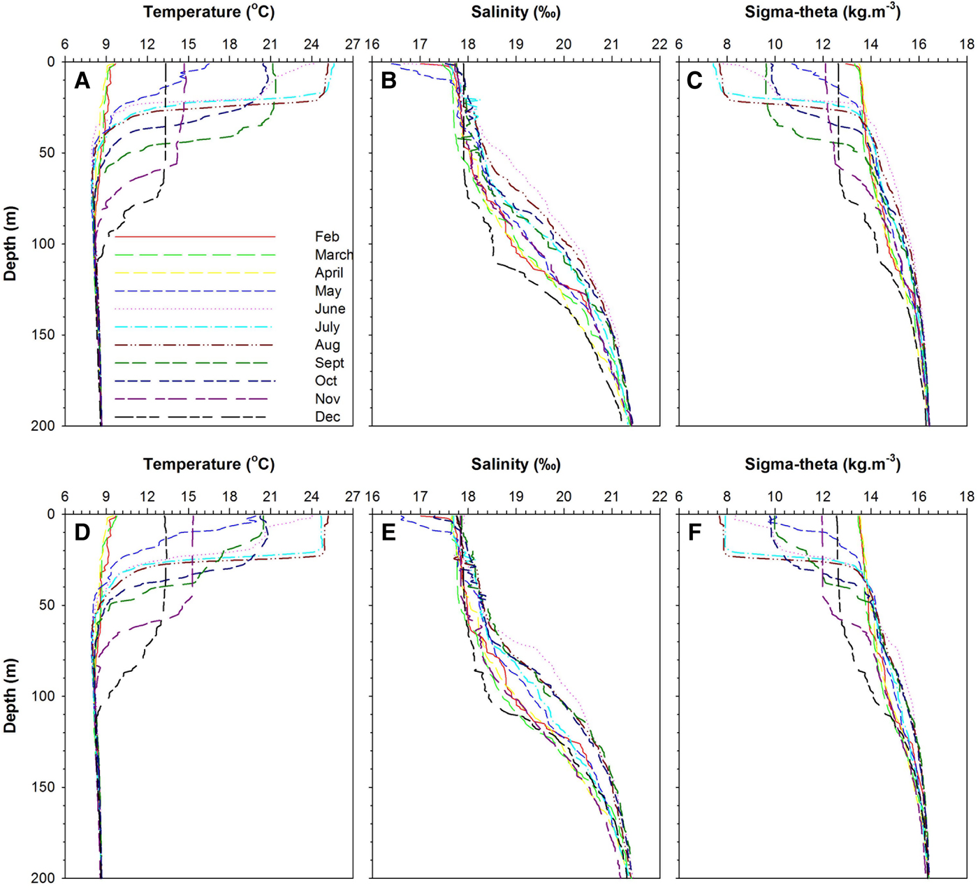
Fig. 2. Temperature, salinity and sigma–theta profiles in the study area: (A–C) coastal station; (D–F) offshore station.
Mixed layer depth and the photic depth are shown in Figure 2. MLD ranged from a maximum of 67 m during December to a minimum of 15 m during June (Figure 3). The euphotic zone depth derived from PAR values varied from 22 to 36 and 21 to 33 m at the coastal and offshore stations, respectively (Figure 3). The photic depth was always deeper than the mixed layer during stratified periods. The water column was strongly stratified during the summer months (15–17 m) as compared to the autumn and winter period (47–67 m). Notably, the whole water column was never completely mixed except in the autumn and winter periods.

Fig. 3. The mixed layer depth (MLD) and photic depth at time of sampling period: (A) coastal station; (B) offshore station.
Nutrients
Extensive vertical mixing during the late winter and early spring resulted in almost a uniform vertical distribution of nutrients (Figure 4). The highest nutrient concentrations were recorded during mixing periods, whereas the lowest ones were observed during stratified periods. The nutricline was generally observed below 30 m during stratified periods. The highest nitrite concentration was measured around 45 m (0.29 µM) and 50 m (0.46 µM) at the coastal and offshore stations, respectively (Figure 4A, B). Among the sampling periods when the data were averaged, the highest nitrite concentration was obtained in March (0.23 µM for the coastal station and 0.33 µM for the offshore station), whereas the lowest (0.02 µM for the coastal station and 0.01 µM for the offshore station) was obtained in July. In general, the average nitrite concentrations for the coastal station (0.07 ± 0.02 µM) were lower than for the offshore station (0.09 ± 0.03 µM).
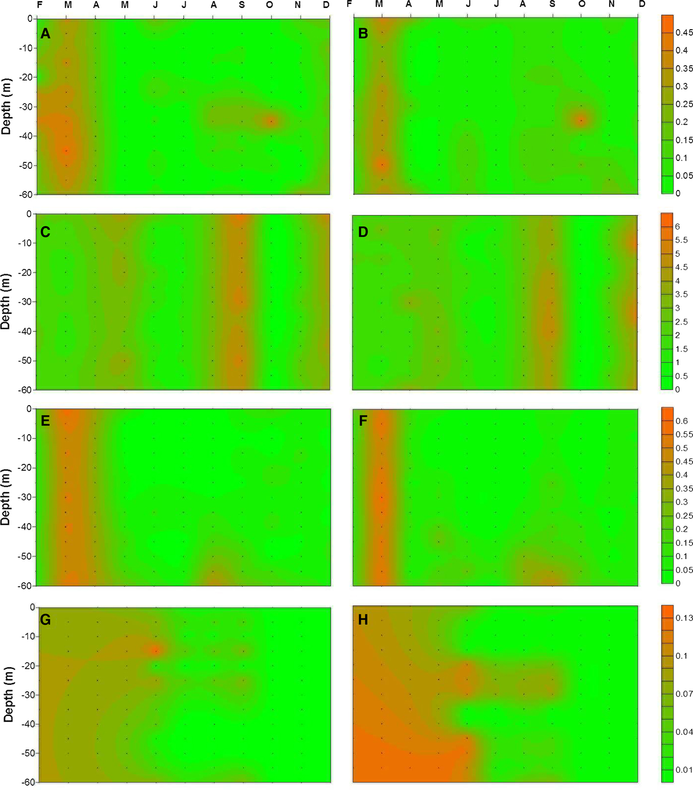
Fig. 4. Nutrient distribution in the upper 60 m in the study area (left and right panel indicate coastal and offshore station, respectively): (A, B) nitrite; (C, D) nitrate; (E, F) silicate; (G, H) phosphate.
Nitrate concentrations followed a similar pattern to nitrite among the stations. The highest concentrations were measured as 5.64 and 5.92 µM around surface waters for the coastal and offshore stations, respectively (Figure 4C, D). The highest concentrations were always recorded in the upper part of the water column and vertically uniform nitrate levels were generally obtained during mixing periods. Overall, the average concentrations were measured as 2.18 (±0.22) μM for the coastal and 2.21 (±0.12) μM for the offshore station. The highest averaged nitrate concentrations were obtained at the surface (2.59 µM) and 30 m (2.42 µM) depths at the coastal and offshore station, respectively. During the sampling period, the lowest averaged nitrate concentrations were recorded as 0.35 µM for the coastal station and 0.31 µM for the offshore station, in October (Figure 4C, D).
Silicate concentrations, shown in Figure 4E, F, increased with depth at the stations. During March an extensive mixing process occurred, substantially characterized by high silicate concentrations. The highest silicate concentrations were obtained at 60 m for both coastal (0.45 µM) and offshore station (0.47 µM), except for March. The average silicate concentration for the coastal station was slightly lower than for the offshore station, except at the surface and 60 m. In general, the average concentrations were obtained as 0.12 (±0.04) and 0.13 (±0.04) μM for coastal and offshore station, respectively. During the sampling period, the highest concentrations were obtained in March (0.50 µM for coastal station and 0.53 µM for offshore station) at both stations. The lowest concentrations were recorded in July.
Throughout the sampling period, phosphate concentrations were always low at the stations. The highest phosphate concentrations were obtained at 15 m (0.04 µM) and 30 m (0.05 µM) depths at the coastal and offshore stations, respectively. Average phosphate concentrations at the coastal station were generally lower than at the offshore station, but not statistically significant (P > 0.05), and recorded as 0.018 (±0.01) and 0.023 (±0.02) μM, respectively. Conversely, the highest concentrations among the months were recorded in June; the lowest concentrations were recorded in December for both stations when compared other nutrient profiles (Figure 4G, H).
The ratio of nutrients (N:P and Si:N, etc.) exhibited vertically different trends between the stations (data not shown). The ratio of N to P at the coastal station was lower than at the offshore station within the first 20 m of the water column. Below this depth, the ratio at the coastal station increased gradually and reached the highest values at 35 m, where the nutricline was observed. Similarly, the ratio of Si to N also increased with depth at the stations.
Phytoplankton
Using microscopy a total of 89 species were identified from both stations throughout the study period (Appendix 3 in supplementary material), 71% of these were dinoflagellate species, 23% were diatom species and 6% consisted of other species, mainly coccolithophores (data not shown). In terms of cell numbers, diatoms dominated, contributing 52.6 and 42.7% of the total phytoplankton cell counts at the coastal and offshore stations, respectively (Table 1). Coccolithophores (entirely made up by E. huxleyi Hay & Mohler) were the second important group in terms of cell count, with an average contribution of 41.5% and 49.6% at the coastal and offshore stations, respectively (Table 1). Despite having a large number of species dinoflagellates, had a low total biomass among the other taxonomic classes. Their contribution varied between 6% and 7.8% at the coastal and offshore stations, respectively.
Table 1. Contribution of different phytoplankton groups to total phytoplankton standing stock and water column averaged cell number in the study area.

ND, no data.
Among the stations diatoms, Coscinodiscus granii Gough, Proboscia alata (Brightwell) Sundström, Pseudosolenia calcaravis Schultze, Thallassionema nitzschioides Mereschkowsky, constituted the highest contribution during May, July and August; coccolithophores were dominant during February, March and December with E. huxleyi present throughout the study (Appendix 3; Figure 5). Dinoflagellates were primarily composed of Alexandrium ostenfeldii Balech & Tangen, A. minutum Halim, Ceratium furca Claparède et Lachmann, C. fusus (Ehrenberg) Dujardin, C. tripos (O.F. Müller) Nitzsch, Dinophysis acuminata Claparède et Lachmann, D. acuta Ehrenberg, D. fortii Pavillard, D. hastata Stein, Gonyaulax spinifera Diesing, Heterocopsa triquetra (Ehrenberg) Stein, Noctiluca scintillans Kofoid et Swezy, Prorocentrum compressum Abé ex Dodge, P. micans Ehrenberg, P. minimum (Pavillard) Schiller, Protoperidinium divergens (Ehrenberg) Balech, P. oblongum Parke et Dodge, P. pallidum (Ostenfeld) Balech and Scrippsiella trochoidea (Stein) Loeblich III, and exhibited almost uniform distribution over all of the study period.

Fig. 5. Monthly and depth dependent average phytoplankton abundance in the study area: (A, C) coastal station; (B, D) offshore station.
The spatio-temporal trend of phytoplankton biomass between the stations is shown in Figure 5. Three phytoplankton blooms (>2.7 × 10⁵ cells l−1) were observed during the study period. The first was a spring bloom of diatoms, Proboscia alata (Brightwell) Sundström, Pseudosolenia calcar-avis Schultze, Pseudo-nitzschia pungens (Grunow ex Cleve) G.R. Hasle; the second, an autumn bloom of coccolithophore E. huxleyi Hay & Mohler; and the third bloom caused by coccolithophore. Coastal and offshore stations exhibited clear bio-geographic differentiation in terms of phytoplankton abundance (cell number) and biomass (phyto-C) (ANOVA, P < 0.05). At the coastal station the highest diatom abundance was recorded in May (3 × 10⁵ cells l−1), while that of coccolithophore E. huxleyi Hay & Mohler was in November (2 × 10⁵ cells l−1). Dinoflagellates were low in terms of abundance among the stations, with a maximum total abundance of 2 × 10⁴ cells l−1. Conversely, at the offshore station, diatoms had higher abundance in May (2 × 10⁵ cells l−1) and September (1.5 × 10⁵ cells l−1) and coccolithophore E. huxleyi Hay & Mohler had higher abundance in February (1.6 × 10⁵ cells l−1) and May (1.2 × 10⁵ cells l−1) (Figure 5A, B).
The phytoplankton abundance profile over the study period is shown in Figure 5C, D. Abundance for all groups was highest in the top 10 m and then declined with depth. At the coastal station, the diatoms were dominant in terms of cell number from the surface to 35 m. Below this depth, coccolithophores (mainly E. huxleyi Hay & Mohler) were the dominant group vertically in the study area. Dinoflagellate abundance profile at the coastal station was generally low. The highest phytoplankton abundance (4.4 × 10⁵ cells l−1) was recorded near the surface at the coastal station. At the offshore station, the highest number of phytoplankton (3 × 10⁵ cells l−1) was obtained at 10 m. The abundance of diatoms and coccolithophores were similar in terms of depth profile at the stations.
Phyto-C and CHEMTAX derived group specific Chl-a
The phyto-C (phytoplankton biomass in terms of carbon) profile for both coastal and offshore stations followed a similar trend as phytoplankton abundance; however temporal differences of the phyto-C were evident. In general, the contribution of diatom-C to the phyto-C was prominent. On the other hand, the contribution of dinoflagellates and coccolithophores to the phyto-C were quite low among the stations (Figure 6). The highest phyto-C values were generally recorded in May, September and October, whereas the lowest ones were obtained during June–August at the coastal station. On the other hand, the highest phyto-C values were measured in May and September at the offshore station. Conversely, the lowest ones were obtained in August and December at the offshore station (Figure 6A, B). Vertically, the upper part of water column was characterized by diatom dominancy at both stations, and declined with depth (Figure 6C, D).

Fig. 6. Monthly and depth dependent average phytoplankton carbon (Phytoplankton-C) distribution in the study area: (A, C) coastal station; (B, D) offshore station.
The average phyto-C for the coastal station (291 ± 66 µg l−1) was slightly greater than for the offshore station (258 ± 35 µg l−1), but not statistically significant (P > 0.05). Overall, the majority of the carbon biomass was represented by diatoms. The contribution of diatoms to total biomass was fairly high, accounted for up to 94% of phyto-C, especially during bloom periods (Table 2). The diatom-C was more strongly correlated with the CHEMTAX-derived diatom-Chl-a at the coastal station (r 2 = 0.85, P < 0.001) than at the offshore station (r 2 = 0.74, P < 0.001) (Figure 7B–F). Coccolithophores, the second most important component of the phytoplankton community (in terms of biomass), contributed up to 75% and 85% of phyto-C at the coastal and offshore station, respectively (Table 2). The correlation between coccolithophore-C and group specific Chl-a for the coastal station (r 2 = 0.84, P < 0.001) was better than for the offshore station (r 2 = 0.71, P < 0.001) (Figure 7D–H). The contribution of dinoflagellate-C to phyto-C was always low (Table 2). The dinoflagellate-C was only strongly correlated with group specific Chl-a at the coastal station (r 2 = 0.80, P < 0.001) (Figure 7C–G). In general, phyto-C and group specific Chl-a exhibited strong correlations among the stations; the correlation for all phytoplankton groups at the coastal station (r 2 = 0.82, P < 0.05) was stronger than at the offshore station (r 2 = 0.77, P < 0.05) (Figure 7).

Fig. 7. Linear relationship between phytoplankton biomass and group specific chlorophyll-a obtained from CHEMTAX with 95% confidence intervals (left and right panel indicate coastal and offshore station, respectively).
Table 2. Water column averaged carbon biomass, % contribution of different phytoplankton groups to total carbon biomass and Phyto-C:Chl-a ratios in the study area.

ND, no data.
The ratio of phyto-C to Chl-a throughout the study period showed similar trend as phyto-C, but there were also major differences over the study period (Table 2). There was a rapid increase in the ratios during May (310 and 308 for coastal and offshore station, respectively), when phytoplankton blooms started in both stations. The highest ratio was observed during summer periods (464 and 421 for coastal and offshore stations, respectively) when the nutrients were depleted during strong stratified periods. The ratios for the coastal station were greater than for the offshore station, but not throughout the study period. On the other hand, the phyto-C profile for diatoms and dinoflagellates rapidly declined after 25–30 m depth; below these depths an increase in coccolithophore-C was observed (data not shown).
Chl-a , pigments and phyto-C
The Chl-a and accessory pigment (e.g. fucoxanthin, peridinin and 19′-hexanoyloxyfucoxanthin) concentrations are shown in Figure 8 and exhibit a high degree of variability. The overall averaged Chl-a concentrations were measured as 1.97 (range 0.52–3.83 µg l−1) and 1.84 µg l−1 (range 0.63–2.55 µg l−1) for the coastal and offshore stations, respectively. The majority of the Chl-a was recorded near the surface (<40 m) in both stations based on vertical distribution. Accessory pigments profiles in the water column exhibited a similar pattern to Chl-a . Fucoxanthin, as expected, was the dominant accessory pigment at the stations. Its concentration within the water column ranged from 0.02 to 3.28 µg l−1 and 0.02 to 2.53 µg l−1 at the coastal and offshore station, respectively. Peridinin concentrations were generally uniform through the water column. The concentrations ranged from 0.03 to 2.55 µg l−1 and 0.03 to 0.72 µg l−1 at the coastal and offshore stations, respectively. The third accessory pigment was 19′- hexanoyloxyfucoxanthin and its concentrations ranged from 0.01 to 1.83 µg l−1 and 0.01 to 1.26 µg l−1 within the water column at the coastal and offshore station, respectively (Figure 8). Other accessory pigments (e.g. diadinoxanthin, zeaxanthin, Chl-b, etc.) were detected at the stations but they were minor and not consistently present; for this reason, the data are not presented. Temporal distribution of pigment concentration was also prominent in the study area. The highest Chl-a concentration was observed during May, September and November at the coastal station. In addition to the mentioned months for the coastal station, the highest Chl-a concentration at the offshore station was also recorded during April.
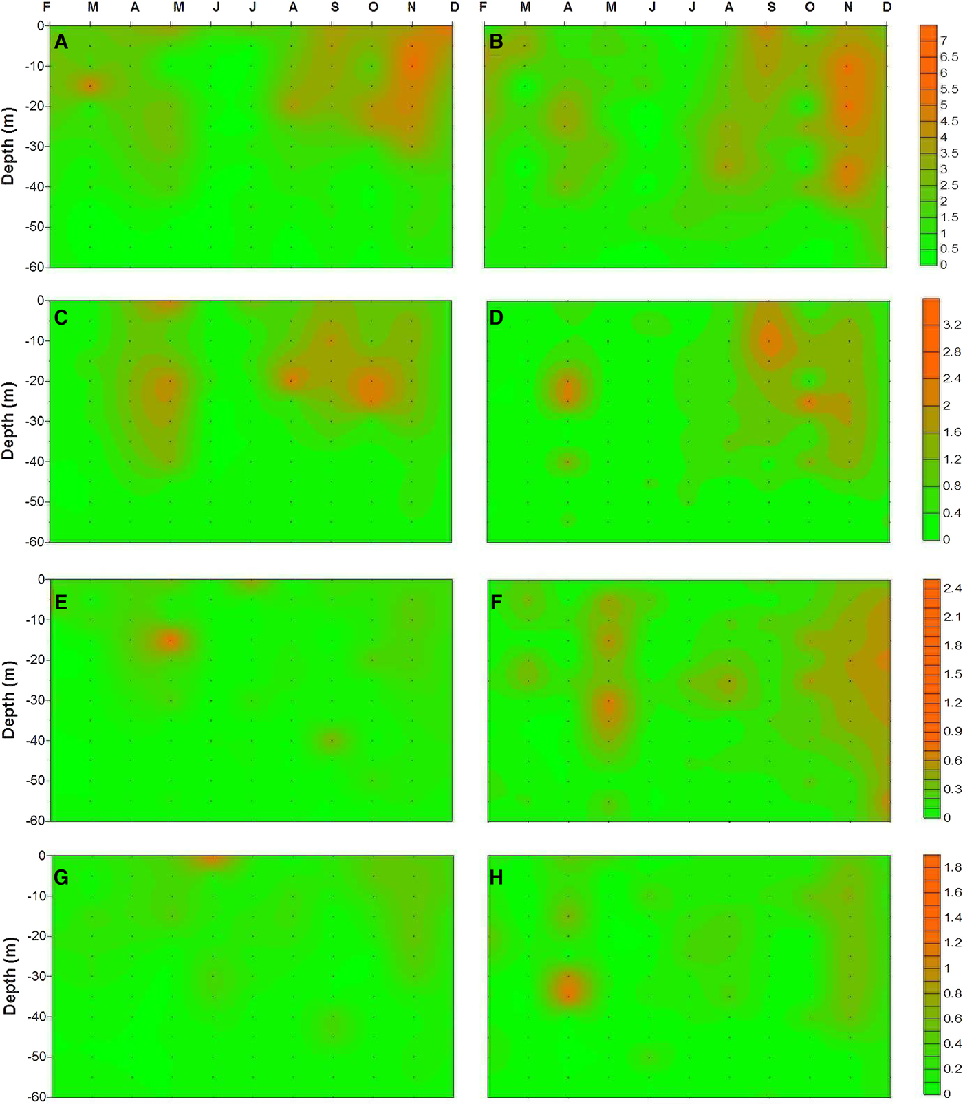
Fig. 8. Pigment distribution in the upper 60 m of water column in the study area (left and right panel indicate coastal and offshore station, respectively: (A, B) Chlorophyll-a; (C, D) fucoxanthin; (E, F) peridinin; (G, H) 19′-hexanoyloxyfucoxanthin.
The differences in pigment distribution were further investigated by using the relationship between phytoplankton biomass (phyto-C) and group specific marker pigment concentrations. The major accessory pigments for the taxonomic groups (i.e. diatoms, dinoflagellates and coccolithophores) showed good correlation with phyto-C. The correlation between diatom-C and fucoxanthin strongly correlated and, the correlation for the offshore station (r 2 = 0.71, P < 0.05) was better than for the coastal station (r 2 = 0.56, P < 0.05). On the other hand, even though diadinoxanthin showed lower concentrations in the study area, the correlation between diatom-C and diadinoxanthin was much better than fucoxanthin (r 2 = 0.85, P < 0.001 for the coastal station and r 2 = 0.91, P < 0.001 for the offshore station) (Figure 9). There was significant correlation between the biomass of dinoflagellates and peridinin (r 2 = 0.88, P < 0.05), particularly at the coastal station. There was also significant correlation between the biomass of E. huxleyi and 19′-hexanoyloxyfucoxanthin for both coastal (r 2 = 0.80, P < 0.05) and offshore (r 2 = 0.71, P < 0.05) stations (Figure 9).
Fig. 9. Linear relationship between phytoplankton groups and marker pigments with 95% confidence intervals: (A, C, E) coastal station; (B, D, F) offshore station.
The measured Chl-a was represented always in higher concentrations at the stations (Figure 10). However, group specific Chl-a concentrations in the area dramatically changed within the water column. The upper part at the coastal station was dominated by higher diatom, chlorophyte-, dinoflagellate- and coccolithophore-specific Chl-a. A similar pattern was also observed at the offshore station. Vertical distribution of diatom and dinoflagellates were nearly similar, but diatom-specific Chl-a concentration was always higher than dinoflagellate-specific Chl-a. On the contrary, coccolithophore-specific Chl-a concentrations were lower concentrations in the area. Other group-specific Chl-a concentrations were generally lower in the study area. Cyanophyte- and chlorophyte-specific Chl-a concentrations were dominant between 15 and 30 m and then declined with depth. Interestingly, chlorophytes were always major groups at the offshore station below the 30 m where deep chlorophyll maximum (DCM) was recorded. There was also DCM at the coastal station (15 m), but it was shallower than at the offshore station. In this study, group-specific contributions of nanoplankton and picoplankton were also first established for the south-eastern part of the Black Sea. Their contributions to total Chl-a were also notably higher in the study area.
Fig. 10. Vertical distribution of chlorophyll-a (Chl-a) (measured) and the group specific Chl-a in the study area: (A) coastal station; (B) offshore station.
DISCUSSION
The results of this study contribute to our understanding of the distribution and composition of major phytoplankton groups, derived from HPLC-based pigment profiles and CHEMTAX analysis, phytoplankton abundance and biomass based on microscopy cell count along the south-eastern coasts of the Black Sea. The present study expands the previous works for the area in terms of studies of HPLC-based pigment profiles and group specific contributions, besides phytoplankton abundance and biomass.
In our study diatoms were found to be the dominant group in terms of biomass, whereas the dinoflagellates showed the highest species diversity. Of the total of 89 species identified, 71% were dinoflagellates, 23% were diatoms and the rest were other groups (mainly coccolithophores). Due to eutrophication which occurred during 1970s and 1980s, the phytoplankton structure (i.e. qualitative and quantitative aspects) drastically changed in the Black Sea (Kideys, Reference Kideys1994; Uysal et al., Reference Uysal, Kideys, Senichkina, Georgieva, Altukhov, Kuzmenko, Manjos, Mutlu, Eker, Ivanov and Oguz1998). Eutrophication caused an increase in bloom frequencies and abundances of many phytoplankton species. In addition the retention of silicate in the dams constructed across rivers (e.g. River Danube) has triggered a change in phytoplankton community composition in favour of coccolithophores and dinoflagellates rather than diatoms post-1970s (Bologa et al., Reference Bologa, Bodeanu, Petran, Tiganus and Zaitsev Yu1995; Cociasu et al., Reference Cociasu, Dorogan, Humborg and Popa1996; Humborg et al., Reference Humborg, Venugopalan, Cociasu and Bodungen1997; Moncheva & Krastev, Reference Moncheva, Krastev, Ozsoy and Mikhaelian1997; Bodeanu et al., Reference Bodeanu, Moncheva, Ruta and Popa1998). Generally, nitrogen and phosphorus are the nutrients increasing with eutrophication, and this increase often leads to excessive phytoplankton growth. However, diatoms require silica for their shells in addition to these nutrients. Because of this, other phytoplankton groups like dinoflagellates and coccolithophores increase in number and biomass in the areas of eutrophication (Escaravage et al., Reference Escaravage, Prins, Nijdam, Smaal and Peeters1999). The contribution of diatoms to total biomass reduced from 92.3% in 1960–1970 to 62.2% in 1983–1988 in the phytoplankton off Romania, and the proportion of dinoflagellates increased from 7.6 to 30.9% in the same periods (Bodeanu, Reference Bodeanu1989). Correspondingly, the species number and abundance of dinoflagellates increased gradually in recent years, and they became the dominant group, especially during the summer months (Ivanov, Reference Ivanov1965; Bologa, Reference Bologa1986; Bodeanu, Reference Bodeanu1989; Karacam & Duzgunes, Reference Karacam and Duzgunes1990; Feyzioglu, Reference Feyzioglu1994; Uysal & Sur, Reference Uysal and Sur1995; Zaitsev & Alexandrov, Reference Zaitsev, Alexandrov, Ozsoy and Mikaelyan1997; Uysal et al., Reference Uysal, Kideys, Senichkina, Georgieva, Altukhov, Kuzmenko, Manjos, Mutlu, Eker, Ivanov and Oguz1998; Moncheva et al., Reference Moncheva, Gotsis-Skretas, Pagou and Krastev2001; Mikaelyan et al., Reference Mikaelyan, Zatsepin and Chasovnikov2013). Bologa (Reference Bologa1986) reported a qualitative change in the phytoplankton groups at the onset of intense eutrophication, when the diatom proportion decreased from 67% (209 species) to 46% (172 species) between 1960–1970 and 1972–1977. Mikaelyan et al. (Reference Mikaelyan, Zatsepin and Chasovnikov2013) also reported that changes in the taxonomic structure of phytoplankton were prominent throughout the period. The contribution of diatoms to the total species number increased from 33% in 1969–1983 to 47% in 1984–1995 and decreased to 31% in 1996–2008. For the same period, dinoflagellate ratios were 58, 36 and 22%, respectively. Coccolithophores increased drastically from 1.3 to 28% for the same period (Mikaelyan et al., Reference Mikaelyan, Zatsepin and Chasovnikov2013). Eker-Develi & Kideys (2003) reported that the contribution of dinoflagellates to the total species number was high in March–April 1995 (41%), October 1995 (44%), April 1996 (45%), June–July 1996 (60%) and April–September 1998 (48%) in the southern Black Sea. In addition, Ediger et al. (Reference Ediger, Soydemir and Kideys2006) reported 62 species, of which 81% were dinoflagellates, 18% were diatoms and 1% were coccolithophores in the south-western Black Sea. Similarly, higher dinoflagellate species dominancy (71% of total species) was also observed in the present study. Our results are consistent with this trend and clearly illustrate that dinoflagellates are becoming the dominant group in terms of species diversity among the stations. Such qualitative changes in the phytoplankton community (i.e. dominancy of dinoflagellates and detecting low biomass communities such as picoplankton) may also imply regime shifts from high trophic level to low trophic level (i.e. the succession, intensity, frequency and extension of phytoplankton blooms, etc.) or cause changes in the lower trophic food web structure in the ecosystem (Oguz, Reference Oguz2005). It is known that dominancy of small-sized phytoplankton groups (e.g. nanoplankton, picoplankton, etc.) indicates mesotrophic and oligotrophic trophic status for a particular area (Aiken et al., Reference Aiken, Pradhan, Barlow, Lavender, Poulton, Holligan and Hardman-Mountford2009).
Analogously, there have also been changes in the dominant phytoplankton species throughout the period. Eker-Develi & Kideys (Reference Eker-Develi and Kideys2003) reported that the most dominant and common species were E. Huxleyi Hay & Mohler, Proboscia alata (Brightwell) Sundström, Chaetoceros curvisetus Cleve, Hillea fusiformis (J. Schiller) J. Schiller, Glenodinium paululum Lindernann, Thalassionema nitzschioides Mereschkowsky, Pseudo-nitzschia pseudodelicatissima (Cleve) Heiden, Pseudosolenia calcar-avis Schultze and Prorocentrum cordatum (Ostenfeld) Dodge, which had high abundances on the southern coast of the Black Sea. In another study, Exuviella cordata, Gyrodinium fusiforme Kofoid & Swezy, Gymnodinium splendens Lebour, Cerataulina bergonii (H. Peragallo) Schütt, Pseudonitzschia delicatissima (Cleve) Heiden and E. huxleyi Hay & Mohler were reported as dominant phytoplankton species (Ediger et al., Reference Ediger, Soydemir and Kideys2006). Our microscopic observations revealed that Proboscia alata (Brightwell) Sundström, Pseudosolenia calcar-avis Schultze, Pseudo-nitzschia pungens (Grunow ex Cleve) G.R. Hasle, Alexandrium minutum Halim, Prorocentrum micans Ehrenberg, P. compressum Abé ex Dodge, P. minimum (Pavillard) Schiller and Emiliania huxleyi Hay & Mohler were the most abundant and prominent species during the study period.
Throughout the study period, total biomass at the coastal station was higher (291 ± 66 µg l−1) than at the offshore station (258 ± 35 µg l−1). Variations in phytoplankton biomass among the different regions of the Black Sea have been reported in previous studies. While the north-western coasts were characterized by high biomass (1000–30,000 µg l−1 (Zaitsev & Alexandrov, Reference Zaitsev, Alexandrov, Ozsoy and Mikaelyan1997)), southern coasts were generally characterized by low biomass (550–1230 µg l−1 and 55–1617 µg l−1 for the south-western and south-eastern Black Sea, respectively (Eker et al., Reference Eker, Georgieva, Senichkina and Kideys1999)). The surface waters of the Black Sea are always poor in nutrients during warm seasons when waters are stratified (Yilmaz et al., Reference Yilmaz, Tugrul, Polat, Ediger, Coban and Morkoc1998). Intense vertical mixing in winter months provides input from the nutricline, which increases surface nitrate concentrations 5–10-fold (Yayla et al., Reference Yayla, Yilmaz and Morkoc2001). In this study, homogeneous nutrient profiles were observed during winter and early spring periods (see also Figure 4). These were also periods when high phytoplankton (especially diatom) abundance and biomass were observed. Diatoms are opportunistic organisms that are able to respond rapidly to nutrient enrichments (e.g. nitrate) (Barlow et al., Reference Barlow, Aiken, Moore, Holligan and Lavender2004). This opportunistic character of diatoms explains the dominance of diatom biomass during mixing periods.
The differences in the biomass between coastal and offshore stations emphasize that physical conditions are the main factors in the study area. Although, Chl-a is widely used as a convenient indicator of phytoplankton biomass, it represents only a small proportion of cellular dry weight and hence carbon content. Carbon content depends on the taxonomic composition of the biomass, the physiological status of the cells and nutrient and light conditions (Gibb et al., Reference Gibb, Barlow, Cummings, Rees, Trees, Holligan and Suggett2000). Studies of micro-algal cultures have shown that the ratio of phyto-C to Chl-a is highly variable, ranging from 18 to 333 (Cloern et al., Reference Cloern, Grenz and Vidergar-Lucas1995), changing in response to irradiance, nutrient availability and temperature. In culture, the ratios are low at low irradiance, high temperatures and under nutrient-replete conditions (Geider, Reference Geider1987). In the present study, great variance was observed in the ratio of phyto-C to Chl-a throughout the study period. The highest ratios were particularly obtained during warm and nutrient-depleted periods (e.g. June and July) when the lowest Chl-a concentrations were measured, whereas the lowest ratios were measured during cold and under non-limiting nutrient periods (see also Table 2). The ratios also declined in line with decreasing irradiance in the water column. Low ratios have also been reported when irradiance is low either during the winter months or at deeper depths in the water column (Llewellyn et al., Reference Llewellyn, Fishwick and Blackford2005). Moreover, high biomass communities (e.g. microplankton) were reported to have lower C:Chl-a ratios than low biomass communities (e.g. picoplankton) in coastal Antarctic waters (Garibotti et al., Reference Garibotti, Vernet, Kozlowski and Ferrario2003). Similarly, the bloom-forming species which dominated during May, July and September may explain relatively low C:Chl-a ratios obtained among the stations. Overall though, the ratios, ranged from 14 to 464, estimated in the present investigation, exhibit an agreement with the literature, which ranges from 36 to 333, (Cloern et al., Reference Cloern, Grenz and Vidergar-Lucas1995; Llewellyn & Gibb (Reference Llewellyn and Gibb2000); Eker-Develi et al., Reference Eker-Develi, Berthon, Canuti, Slabakova, Moncheva, Shtereva and Dzhurova2012).
In the seasonally stratified surface waters of the Black Sea, Chl-a profiles display a sub-surface maximum at the base of the euphotic zone (Coban-Yildiz et al., Reference Coban-Yildiz, Tugrul, Ediger, Yilmaz and Polat2000). It was reported that the concentrations in the euphotic zone were generally low (<0.5 µg l−1), with the lowest values in the surface mixed layer, and a subsurface Chl-a maximum formed near the base of the euphotic zone and/or below the seasonal thermocline, corresponding to depths receiving 0.5–2% of the surface light (Yilmaz et al., Reference Yilmaz, Tugrul, Polat, Ediger, Coban and Morkoc1998). Besides, the average Chl-a concentration for the southern Black Sea within the euphotic zone has been reported as 0.1–1.5 µg l−1 during the spring–autumn period of 1995–1996 (Yilmaz et al., Reference Yilmaz, Tugrul, Polat, Ediger, Coban and Morkoc1998). In the present study, Chl-a values were significantly different between coastal and offshore stations (ANOVA, P < 0.01). High concentrations (>2 µg l−1) were observed up to 30 and 35 m depth at the coastal and offshore stations, respectively. The DCM was formed near the euphotic zone in the present study, similar to previous studies. Earlier investigations indicated that prochlorophytes and cyanophytes dominate in the upper mixed layer, while pico- and nanoeukaryotes constitute a high portion of phytoplankton at the DCM (Perez et al., Reference Perez, Fernandez, Maranon, Moran and Zubkov2006). Chlorophytes and cyanophytes were dominant at the DCM in the present study. Claustre & Marthy (Reference Claustre and Marthy1995) reported that a deep nanoflagellate population (i.e. chlorophytes and prymnesiophytes) can develop close to the nutricline at very low light levels. The reasons for the existence of nanoplankton at the DCM are still unclear (Ras et al., Reference Ras, Claustre and Uitz2008). However, several mechanism have been proposed to explain its formation and maintenance, including higher in situ growth at the nutricline, physiological acclimation to low irradiance and high nutrient concentration, accumulation of sinking phytoplankton, behavioural aggregation of phytoplankton groups and differential grazing pattern on the phytoplankton communities (Perez et al., Reference Perez, Fernandez, Maranon, Moran and Zubkov2006). Cermeno et al. (Reference Cermeno, Dutkiewiczb, Harrisc, Followsb, Schofielda and Falkowski2008) also reported that coccolithophorids may increase rapidly in abundance relative to diatoms as the water column stratifies and the nutricline deepens. Moreover, Kopuz et al. (Reference Kopuz, Feyzioglu and Agirbas2012) reported that picoplankton constituted the major part of the phytoplankton communities at 1% light intensities during June 2010 for the south-eastern Black Sea. All these statements support the dominancy of pico- and nanoeukaryotes at the DCM in the study area.
The CHEMTAX analysis also provided the contribution of other phytoplankton groups (e.g. pico- and nanoplankton which cannot be completely identified under the microscope) to total phytoplankton biomass. Especially, cyanophytes and chlorophytes prevailed in the DCM layer at the stations. There was also a strong relationship between dinoflagellate-C and peridinin, except for the offshore station. We also observed a significant correlation between dinoflagellate-C and diadinoxanthin (r 2 = 0.59, P < 0.05 for the coastal station and r 2 = 0.64, P < 0.05 for the offshore station) and between dinoflagellate-C and 19′-hexanoyloxyfucoxanthin (r 2 = 0.55, P < 0.05 for the offshore station) in the study area. Moreover, there was a strong correlation between coccolithophore-C and 19′-hexanoyloxyfucoxanthin. It could be possible that some dinoflagellate species contain 19′-hexanoyloxyfucoxanthin. Eker-Develi et al. (Reference Eker-Develi, Berthon, Canuti, Slabakova, Moncheva, Shtereva and Dzhurova2012) also reported high 19-Hex concentrations corresponding to high dinoflagellate-C from the north-western Black Sea. 19′-hexanoyloxyfucoxanthin and fucoxanthin-containing dinoflagellates have been reported in the English Channel previously (Irigoien et al., Reference Irigoien, Meyer, Harris and Harbour2004). It is difficult to distinguish autotrophic, heterotrophic and mix-otrophic dinoflagellates by microscope, whereas the HPLC method may facilitate the estimations, since pigment contents are measured (Llewellyn et al., Reference Llewellyn, Fishwick and Blackford2005). There are still certain discrepancies in using diagnostic pigments to infer phytoplankton functional types, and as stated by Vidussi et al. (Reference Vidussi, Claustre, Manca, Luchetta and Marty2001), some diagnostic pigments such as fucoxanthin (main indicator of diatoms) may also be found in some flagellates. The pigment grouping, therefore, does not strictly reflect true size of phytoplankton communities, and phytoplankton functional types derived from the diagnostic pigments are indicative but not definitive (Brewin et al., Reference Brewin, Sathyendranath, Hirata, Lavender, Barciela and Hardman-Mountford2010). It should be noted that group specific Chl-a was calculated using different matrices for different groups of samples as determined by CHEMTAX pigment analysis. This allowed better correlation than using the raw pigment data (see also Figures 7 and 9). The results obtained in the present study bring a more complete comprehensive picture of the composition of the phytoplankton population for the study area and also imply that microscopic investigation should be accompanied by CHEMTAX analysis.
In the present investigation, nutrient concentrations were slightly different between the stations, but not statistically significant (P > 0.05). However, high pigment concentrations recorded during extensive vertical mixing periods lead to high diatom and dinoflagellate abundance at the stations (see also Figure 5). It is known that coccolithophores and diatoms dominate the base of the food web in temperate marine waters. Especially diatoms have high abundance in nutrient-enriched waters (e.g. upwelling areas and coastal waters) and at the onset of the spring bloom. After the spring bloom, nitrate and silicate were depleted and small-sized groups and prymnesiophytes dominated in the upper water column (Llewellyn & Gibb, Reference Llewellyn and Gibb2000). It is conceivable that the positive relationship reported here between the nutricline depth and the coccolithophore-to-diatom ratio could be driven by differences in the silicate-to-nitrate input ratio at the base of the thermocline (Cermeno et al., Reference Cermeno, Dutkiewiczb, Harrisc, Followsb, Schofielda and Falkowski2008). However, assuming that coccolithophorids are more efficient than diatoms in nutrient acquisition at low concentrations (Litchman et al., Reference Litchman, Klausmeier, Schofield and Falkowski2007; Iglesias-Rodriguez et al., Reference Iglesias-Rodriguez, Halloran, Rickaby, Hall, Colmenero-Hidalgo, Gittins, Green, Tyrrell, Gibbs, von Dassow, Rehm, Armbrust and Boessenkool2008), an increase in the silicate-to-nitrate input ratio would decrease the coccolithophore-to-diatom ratio (Cermeno et al., Reference Cermeno, Dutkiewiczb, Harrisc, Followsb, Schofielda and Falkowski2008). A spring bloom of diatoms and an autumn bloom of coccolithophore were observed in the present study. The findings also concur with the contribution of group specific pigment to Chl-a concentration. The impact of nutrient limitation on the competitive success of diatoms and coccolithophorids also has profound implications (Cermeno et al., Reference Cermeno, Dutkiewiczb, Harrisc, Followsb, Schofielda and Falkowski2008).
Diatoms were the main group in terms of group-specific contribution to Chl-a at both coastal and offshore station. Dinoflagellates were the second dominant group at the coastal station, whereas coccolithophores were the main group at the offshore station. The relationship between marker pigment and Chl-a varies for the different algal groups and also among the species of the same groups (Millie et al., Reference Millie, Paerl, Hurley, Kirkpatrick and Menon1993). The group specific Chl-a profile was different within the water column; while diatoms were main group up to 35 m depth, cyanophytes and chlorophytes were the dominant group below this depths. During the study period, the ratio of N to P revealed different profiles. Especially, below 30 m, the ratios were prominent which indicates the nutricline formation. These depths were below the euphotic zone (30 m) and richer in terms of nutrient concentrations (see also Figure 4). It is well known that E. huxleyi Hay & Mohler becomes more abundant at high N:P ratio (Riegman & Kraay, Reference Riegman and Kraay2001; Ediger et al., Reference Ediger, Soydemir and Kideys2006) but at low irradiance compensation (Riegman & Kraay, Reference Riegman and Kraay2001; Haxo, Reference Haxo2004). The reason for having a high quantity of coccolithophores below 35 m at the stations may be due to these factors.
CONCLUDING REMARKS
The present study allowed us to examine the spatio-temporal distribution and composition of phytoplankton groups via CHEMTAX pigment analysis and microscopy cell count along the south-eastern coasts of the Black Sea. Thanks to detailed pigment data and microscopic examination, the study improves our ability to assess the current status of the coastal and offshore phytoplankton community from many aspects (e.g. Chl-a, group specific Chl-a, pigments, phyto-C, nutrients, light, etc.) for the study area. Limited investigations for the study area have not allowed for long-term comparisons with other parts of the Black Sea. Improving the long-term understanding of changes in pelagic ecosystem is only possible via continuous monitoring programmes. In this regard, the present study undoubtedly documents that the study area needs such programmes.
Comparative studies generally show good agreement between the two techniques for large diatoms, but the agreement is poorer for dinoflagellates, prymnesiophytes and small flagellates, due to ambiguous or shared marker pigments (Wright et al., Reference Wright, Thomas, Marchant, Higgins, Mackey and Mackey1996; Jeffrey & Vesk, Reference Jeffrey, Vesk, Jeffrey, Mantoura and Wright1997; Irigoien et al., Reference Irigoien, Meyer, Harris and Harbour2004; Zapata et al., Reference Zapata, Jeffrey, Wright, Rodríguez, Garrido and Clementson2004; Eker-Develi et al., Reference Eker-Develi, Berthon and Linde2008, Reference Eker-Develi, Berthon, Canuti, Slabakova, Moncheva, Shtereva and Dzhurova2012). Due to the ambiguity of some marker pigments, HPLC-pigment analysis should be used supplementary to microscopy analysis to identify the species (Mackey et al., Reference Mackey, Mackey, Higgins and Wright1996; Llewellyn et al., Reference Llewellyn, Fishwick and Blackford2005; Eker-Develi et al., Reference Eker-Develi, Berthon, Canuti, Slabakova, Moncheva, Shtereva and Dzhurova2012). In general, no single technique or methodology is ideal for resolving phytoplankton community structure and dynamics. Thus, the role of HPLC-based pigment analyses for quantitatively assessing phytoplankton composition should be considered as complementary to microscopy analyses, and not an exclusive replacement for microscopic enumeration.
In conclusion, the combination of HPLC-based pigment analysis and microscopic phytoplankton enumeration provided detailed information about the state of the phytoplankton community composition on the south-eastern coasts of the Black Sea. Besides, and using CHEMTAX analysis improved interpretation of pigment data in terms of different phytoplankton groups (e.g. micro-, nano- and picophytoplankton) in the study area. Moreover, this is the first study comparing group specific Chl-a and carbon biomass by using CHEMTAX and microscopic examination for the study area. This research may be helpful for future investigations to ascertain and evaluate the changes in the structure of the Black Sea ecosystem.
ACKNOWLEDGEMENTS
We thank the crew of RV ‘Denar I’ for their assistance during the cruise, Dilek Ediger and Serkan Koral for HPLC analyses. The authors would also like to thank Dr Elif Eker-Develi for her helpful comments on the evolution of the manuscript.
FINANCIAL SUPPORT
This work was funded by the Scientific and Technological Research Council of Turkey (TUBITAK, Project No: 108Y241).
Supplementary materials and methods
The supplementary material for this article can be found at http://www.journals.cambridge.org/MBI


