1. Introduction
The idea of the Keynesian multiplier is revisited here. However, besides a review of the perspective of economic thought, we suggest a focused discussion on the effects of a special type of transfer observed in Portugal, i.e., pensions. We do not restrict our analysis to the macroeconomic effects of pensions on national income but rather take a more in-depth approach. In this work, we study the effects of the pensions received in each Portuguese municipality not only on the purchasing power of that municipality but also on the surrounding areas’ levels of purchasing power.
We know that pensions are attributed to certain persons under the basic motivation of a compensation for their loss of productivity or under the justification of being a payment to retired citizens who contributed to the aforementioned pension system during their active working lives. However, until now, there has not been a substantial discussion about the effects of pensions on surrounding places or in the self-economy, either in Portugal or other countries.
We find some rationale for this apparent lack of interest in the low value of pensions in the first times of the theoretical dominance of the models of aggregate expenditures (from 1960s onward). But nowadays the value of pensions is substantially higher in most developed economies. Thus, today's relevance recognizes a complex set of challenges emerging from the changed mobility of pensioners (from low mobility that characterized pensioners from rural areas several decades ago to the high mobility of most pensioners now) and extends to other challenges, such as the multiplier effects in local economies and/or in the surrounding areas, the possibility of leakage situations, and the influence of the evolution of the values of pensions in the level of aggregate welfare. We aim to address these issues in the present paper.
The structure of this work is as follows. Section 2 describes the importance of pensions in the Portuguese system of social security. It also describes the theoretical models behind the use of transfers and pensions as components of the equation of aggregate expenditures observed in each Portuguese municipality. Then, we explore a model derived from the one developed by Haining (Reference Haining1987), which links the previous discussion to the possibility of studying spillover effects that result from changes in pensions observed in a certain area. Section 3 explores several empirical models studied in the literature of spatial economics (e.g., the Dynamic Spatial Durbin Model (DSDM) or the Dynamic Spatial Error Model (DSEM)) and presents a more-detailed discussion about the estimates we acquired. Finally, Section 4 concludes the paper and offers suggestions about the possibilities of further work in the field.
2. A review of the literature – from the distribution of pensions across the Portuguese territory to their effects on local economies
At the present time, the elderly population (over 65 years old) is one of the main focuses of social science research across the world. In regard to this topic, Portugal has seen its total population growing at a slower pace, about 19.46% between 1970 and 2016. Meanwhile, the current proportion of elderly Portuguese compared with the total population has increased at a significant rate; this value is approximately 20.91% in contrast to 65.03% of working age people. Over 45 years, Portugal has seen its elderly population increase by 158.20% (from 836,058 in 1971 to 2,158,733 in 2016) compared with a 41.10% decline in the number of young people (<15 years old). These values are consequences of the decrease in family size, a decline in the fertility rate (1.36% in 2016), and an increase in life expectancy (80.60 years in 2016).
These demographic changes have become a matter of concern for governments. Considering the Portuguese data for 2015, the total amount of money used to pay pensions, as indicated in the nation's Social Security report, was 15,753.2 million euros. These pensions were divided as survival pensions (2,174 million euros), disability pensions (1,302 million euros), and old age pensions (12,275 million euros), which represent a weight of 32.49% in the country's total public expenditures.
By examining Figure 1, we can see that the average value of pensions in 2015 was not the same across the different municipalities of the continental part of the country. There is a concentration of the highest values on the coastal side of Portugal, while the interior municipalities are characterized by lower values. An additional observation that emerges is that the main cities of each district (usually the administrative capital and surrounding municipalities) received a higher average monetary value.

Figure 1. (Colour online) Average value of pensions by Portuguese municipality, 2015.
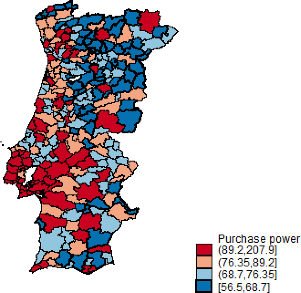
Besides these preliminary descriptive observations, we want to analyze how Figure 1 can be related to Figure 2, which shows the spatial distribution of the level of purchasing power across the Portuguese municipalities in the year of 2015.

Figure 2. (Colour online) Purchase power by Portuguese municipality, 2015.
Figure 2 also reveals a concentration of the purchasing power estimated for Portuguese municipalities in certain cases. These cases tend to be located on the coastal side of the country or in the main cities of the interior.
Therefore, our aim is to develop this study motivated by two stimuli. The first is the intention to study the geographic dispersion of pensions in Portugal, an original topic in the literature. This will enlighten us about the effectiveness of the redistribution purposes of the Portuguese pension scheme and about the spatial autocorrelation of these flows. The second motivation involves the opportunity to detail the effects of pension distributions on the level of purchasing power observed in Portuguese municipalities. Besides revisiting the Keynesian model for the aggregate expenditure, we will include the possibility of spillover effects from neighboring municipalities’ levels of pensions on the observed value of purchasing power for each municipality.
2.1 Modeling the income of a Portuguese municipality in regard to pensions received
The pensions received by individuals tend to be a share of their median wages. This is associated with reduced purchasing power for pensioners compared with wage earners (Hardy, Reference Hardy and Uhlenberg2009). However, we are interested in investigating how the evolution of the levels of pensions received by Portuguese pensioners affects the purchasing power of the surrounding economy. For details of this analysis, we begin with a standard model of aggregate expenditure (Simões Lopes, Reference Simões Lopes1979; Zanglein, Reference Zanglein2005; Mulvey and Purcell, Reference Mulvey and Purcell2008). We model the basic income expenditure identity for a given Portuguese locale, e.g., for a given municipality, using the equation below:
 $$Y = AE = C + I + G + \lpar {X\ndash M} \rpar $$
In equation (1), Y identifies the regional income, which is assumed to be identical to the aggregate expenditure; C, the regional consumption; I, the regional investment; G, the public expenditure in the region; X, the regional exports; and M, the regional imports.
There have already been robust discussions focused on the appropriateness and properties of the Keynesian aggregate expenditure model (Ritter and Leijonhufvud, Reference Ritter and Leijonhufvud1970; Rutherford and Desroches, Reference Rutherford and Desroches2008; Dosi et al., Reference Dosi, Pereira, Roventini and Virgillito2017). We recall a few of assumptions here. C, the regional consumption function, is derived by  $C = \bar{C} + c*Yd$, meaning that C results from the sum of an autonomous level of consumption,
  $\bar{C}$, plus the product of the marginal propensity to consume, c, and the disposable income, Yd. Disposable income is identified as available income after tax collection (T) and the reception of transfers (R). Let us also assume that the value of pensions (P) over the transfers (R) observed in an economy described by our model is p, i.e., p = P/R. For simplicity, we will assume that the levels of investment, public spending, and regional exports are exogenously determined:
  $I = \bar{I},\;G = \bar{G}$, and
  $X = \bar{X}$. Regional imports are, typically, assumed to be dependent on the level of regional income besides an exogenous component,
  $M = \bar{M} + mY$. Therefore, the autonomous regional spending is determined by finding the sum of
  $\bar{I},\bar{G}$ and by the exogenous current account:
  $\bar{X}-\bar{M}$.
2.2 The effects of pensions on the local economy
Pensions exert effects in three major dimensions of the local economy. The literature (Mulvey and Purcell, Reference Mulvey and Purcell2008; Kuivalainen et al., Reference Kuivalainen, Rantala, Ahonen, Kuitto and Palomäki2017) has identified these as: a positive increase in the levels of consumption, redistributive effects, and positive impacts on the welfare of the society. We will comment on these.
The effect on consumption has been analyzed by authors including Kuivalainen et al. (Reference Kuivalainen, Rantala, Ahonen, Kuitto and Palomäki2017). Pensions are assumed as net transfers from the government to individuals, thereby increasing their own endowments. These individuals will spend their endowments in consumption, saving the resulting difference between the afforded income and the consumption expenditures. Given the levels of the afforded income characterizing pensioners, most of it goes for consumption (Knutsen and Rasmussen, Reference Knutsen and Rasmussen2017), and because of their preferences as well as their restrictions, this income tends to be spent within the regional economy, as additionally discussed by Gurria et al. (Reference Gurria, Nieto, Hernandez and Frutos2013).
The redistributive effects also have a long record of analysis. Resulting from the work of Burda and Wyplosz (Reference Burda and Wyplosz1993), pensions have been considered as redistributive tools, currently funded by the wealthiest groups of individuals and favoring those who, because of retirement or diminished capacities for working or because of social exclusion, are not able to afford higher levels of endowments.
Finally, as an ultimate consequence, research by Mulvey and Purcell (Reference Mulvey and Purcell2008) has revealed positive effects of pensions on the welfare of the society. The increase in consumption levels combined with the reduction of inequality tends to improve living standards more visibly in low-income groups (Azevedo et al., Reference Azevedo, Inchauste and Sanfelice2013; Rodrigues and Andrade, Reference Rodrigues and Andrade2014). Additionally, Diris et al. (Reference Diris, Vandenbroucke and Verbist2017) have argued that (effective) increases in the value of pensions contribute to increasing the dynamics of social capital and the social dynamism of pensioners, their families, and their relatives, which in turn has non-negligible impacts on the economy in terms of welfare measures.
Pensions have also given rise to three major concerns in the literature. The first line of criticism regards the non-linearity of pensions’ effects in the levels of productivity. At first glance, the inflows generated by pensions could be considered as improving the level of expenditures and thus contributing to increases in the level of aggregate income. However, the research of Reil-Held (Reference Reil-Held2006) and Fan (Reference Fan2010) revealed the existence of a significant probability of a kind of ‘crowding-out effect’ – that is, higher levels of pensions can deter the presence in the workforce of some (eligible) workers who prefer to receive pensions rather than salaries. If the individual productivity level of these workers is low, their move to the group of pensioners will raise overall productivity. However, if the individual productivity level of these eligible workers is high, their move to the group of pensioners will tend to diminish overall productivity.
The second concern is related to sustainability. The different schemes adopted predominantly in countries after the Second World War have faced an increasing number of concerns in regard to the sustainability of pension schemes. The works of Ebbinghaus and Gronwald (Reference Ebbinghaus, Gronwald and Ebbinghaus2011) clearly detailed these concerns. Since pressures originating with the decreasing numbers of people in the workforce compared with the increasing numbers of pensioners have resulted in necessary changes in regard to the age of retirement or to the value-to-date of the expected pension amounts, there are many concerns linked directly to the sustainability of pension systems.
Finally, the concern regarding social instability claims that deep imbalances (stemming from the issue of the sustainability of pension systems) may lead to generalized dissatisfaction among the different cohorts of people in the population: workers versus pensioners, young versus older people, etc. This turmoil may, in turn, contribute to a context of political instability having potentially significant consequences on the economic growth path of economies (Chen et al., Reference Chen, Lesson, Han and You2017).
Recalling the model suggested by equation (1), we observe the multiplier effect of a unit increase in pensions using the following equation:
 $$\displaystyle{{\partial Y} \over {\partial P}} = \displaystyle{{c{^\ast}p} \over {1 + m-c{^\ast}(1-t)}}.$$
 This is lower than the standard Keynesian multiplier of transfer payments (because p tends to be lower than 1),  $\displaystyle{{\partial Y} \over {\partial R}} = \displaystyle{c \over {1 + m-c*(1-t)}}.$
Therefore, as p increases the multiplier effect of pensions will converge to the multiplier effect of transfer payments.
2.3 The effects of pensions on neighboring economies – income leakages, regional imports, and intra household redistribution
The effects of pensions on local economies suggested by equation (2) can also be distorted and/or affected by three sources of (income) leakages (Burda and Wyplosz, Reference Burda and Wyplosz1993: 212): unproductive savings, budget surpluses, and spending away from the hosting economy. The first of these sources is unproductive savings. As part of the income is spent, it is expected that the remaining saved part returns to the economic system via financial institutions. However, various studies have proven that this may be not the case. Part of the remaining saved income may be not put into banks (Zadoia, Reference Zadoia2017; Zaghdoudi and Maktouf, Reference Zaghdoudi and Maktouf2017) in certain circumstances (e.g., banking crises, an urgent need for liquidity by the household, etc.), or the role of the financial institutions may not be very effective, as the models have suggested (problems with banks’ governance, bank defaults, money laundering, etc.). As a consequence, local income leaks, and this leakage weakens the key parameters of the demand multiplier. Particular situations relating pensions to this source of leakage have been discussed by Zaghdoudi and Maktouf (Reference Zaghdoudi and Maktouf2017) and by Zadoia (Reference Zadoia2017).
A second source relates to budget surpluses (Razin and Sadka, Reference Razin and Sadka2007). Increases in aggregate demand may be captured first by taxes (and not by government spending), also contributing to a decrease in the ultimate demand multiplier (Marcis and Veseth, Reference Marcis, Veseth and Veseth1981). Finally, the third type of leakage has its origins in the rapid growth that has been observed as being significantly correlated with a deterioration of the current account of an economy (Das, Reference Das2016). This also deserves to be discussed in light of Portuguese pensioners and the recent evolution of pensions. Pensioners are now more mobile than they were several decades ago, and a number of studies identify the roles of programs referred to as ‘senior tourism’ or ‘social tourism’, the improvement in the quality of roads (Sebova et al., Reference Sebova, Marcekova and Simockova2016), and the increasing autonomy of aging pensioners (Popov et al., Reference Popov, Chigisheva, Nikitina and Vorontsova2015). This additional source of income leakage means that there have been more instances of Portuguese pensioners spending their endowments in goods and services classified as ‘regional imports’, i.e., goods and services produced outside the region in which the Portuguese pensioners reside.
There is also a second dimension suggesting that pensioners are contributing more to regional imports than in the past. One of the economic effects of pensions regards intra household redistribution (Dasgupta, 2011); according to this, pensioners of a household/region are able to give part of the money they receive as a pension to their children or other relatives. Therefore, even if the consumption of pensioners tends to be more static and concentrated in the areas where they reside, their children or other family members who receive money from pensioners may spend it in different markets, i.e., beyond the pensioner's economic boundaries.
Therefore, in the next section, we will discuss a model based on the work of Haining (Reference Haining1987) in order to explore the effects of Portuguese pensions on the purchasing power of a region (comprising the municipality of the pensioner plus the surrounding and neighboring municipalities).
2.4 Toward a model of the spillover effects of pensions – revisiting Haining (Reference Haining1987)
To analytically discuss pension leakages due to the third channel – the openness of a local/regional economy to neighboring spaces – we will continue to base our analysis on the (Keynesian) model of regional demand. The use of such models in regional economics is not a novelty. Work by Haining (Reference Haining1987) and a robust line of derivative research have already explored, discussed, and revised the possibility of flows of income among contiguous regions.
Haining's (Reference Haining1987) work is important in this debate (Griffith et al., Reference Griffith, Chun, O'Kelly, Berry, Haining and Kwan2012), as it was the first to analyze income flows between contiguous areas. In a work published a year earlier, Haining (Reference Haining1986) had already referred to Keynesian models, in which community income was divided into exogenous and endogenous components, with the exogenous component further partitioned into interregional and intercommunity scales of income transfer. Haining (Reference Haining1987) considered not only static models but also analyzed temporal income diffusion models. Finally, he also detailed key economic parameters in these models, namely, propensities to spend locally and to spend non-locally (1987).
Haining's (Reference Haining1987) static model was inspired by Beckmann (Reference Beckmann, Kuhn and Szego1971). It starts by studying the effects of spatial redistribution on income, Y, on a spatially specific exogenously given injection, X (equation (3)):
 $$Y = [I-\Omega ]^{-1}X$$
The model is then derived to obtain equation (4):
 $$Y = \lpar {c\ndash d} \rpar Y + mWY + X$$
In equation (4), c identifies the (Keynesian) propensity to spend and d is a measure of the propensity to spend non-locally. As a consequence, Haining (Reference Haining1987) interpreted the parameter (c − d) as the income creating a local propensity to consume in the area where the income was received. The parameter m in equation (4) refers to the propensity for a unit of income in a neighboring area, j, to create income in the analyzed area, i. W is a connectivity matrix with the j-th row all zeros except in those positions corresponding to the neighbors of i.
Haining (Reference Haining1987) also studied the temporal version of these models. Assuming that consumption expenditures are lagged functions of income, the previous equation (3) can be extended to the system of equations (5) and (6):
 $$Y_t = {\rm} X_t + C_t$$
 $$C_t = \Omega Y_{t-1}$$
The one-dimensional version of the model is
 $$Y_{i,t} = \lpar {c-d} \rpar Y_{i,t-1} + m\lsqb {Y_{i-1,t-1} + Y_{i + 1,t-1}} \rsqb + X_{i,t}$$
After analyzing the Green functions for the temporal income model, Haining (Reference Haining1987) observed that, as (c–d) increases, the timing of the peak effect is delayed for a given m and for a given distance, and as m increases, the timing of the peak effect is brought forward for a fixed (c − d) and for a given distance between the areas of study.
Empirical attempts that properly recognize the work of Haining (Reference Haining1987) have been undertaken by Biles (Reference Biles2003), Tirtiroğlu et al. (Reference Tırtıroğlu, Tanyeri, Tırtıroğlu and Daniels2012), and Gatzlaff and Tirtiroglou (Reference Gatzlaff and Tirtiroglou1995).
Gatzlaff and Tirtiroglou (Reference Gatzlaff and Tirtiroglou1995) referred to Haining (Reference Haining1987) to support an analysis of the values and prices associated with real estate market segments. These authors detailed the degrees of efficiency in three segments: housing, income property, and land markets. Biles (Reference Biles2003) extended Haining's (Reference Haining1987) discussion to a multi-region context in order to analyze feedback effects. An additional feature in Biles's (Reference Biles2003) framework relates to a formal assessment of variation in the magnitude of regional multipliers. The work of Tirtiroğlu et al. (Reference Tırtıroğlu, Tanyeri, Tırtıroğlu and Daniels2012) empirically examined cross-fertilization in the productivity growth of banks among neighboring and non-neighboring North American states. This analysis was run considering specific periods of banking deregulation.
Overall, these three studies (Gatzlaff and Tirtiroglou, Reference Gatzlaff and Tirtiroglou1995; Biles, Reference Biles2003; Tirtiroğlu et al., Reference Tırtıroğlu, Tanyeri, Tırtıroğlu and Daniels2012) identified the presence of positive flows of incomes across neighboring areas and that the contagious effects of exogenous shocks that happen in one region are also realized in the reactive dimensions observed for other regions.
The STAR models (smooth transition autoregressive models) are a new generation of models inspired by the possibility of using the temporal and spatial autocorrelation of the income of a given place as regressors. From the work of Terasvirta and Anderson (Reference Terasvirta and Anderson1992) to the work of Pede et al. (Reference Pede, Florax and Holt2008), a diversity of research has appeared.
Following the works of previously mentioned authors, our equation (1) must include the spillover effects, either as endogenous effects or exogenous interactions:
 $$Y_{i,t} = C_{i,t} + I_{i,t} + G_{i,t} + \rho (X_{i,t}-M_{i,t})$$
In equation (8), Y i,t still identifies the regional income and C i,t the consumption level, and I i,t and G i,t still identify the regional investment and the public expenditure in the region, respectively. The regional exports are represented by X; the regional imports by M; and ρ represents the parameter for the neighborhood's influence, meaning that higher values for ρ magnify the value of the current account (either by increasing the current account's surplus or by reducing the current account's deficit). If ρ = 0, the observed space can be identified to a close economy.
Following the assumptions identified for equation (1), we highlight that the exogenous current account is now multiplied by the neighborhood parameter:  $\rho *(\bar{X}-\bar{M})$. This slightly changes the multiplier for the pensions toward equation (9):
 $$\displaystyle{{\partial Y} \over {\partial P}} = \displaystyle{{c{^\ast}p} \over {1 + \rho {^\ast}m-c{^\ast}(1-t)}}$$
Equation (9) reveals a multiplier that has a lower effect on income than the multiplier in equation (2). This fact favors the hypothesis of higher leakages in income when the neighborhood has higher influence (Herz and Hohberger, Reference Herz and Hohberger2013).
We can explore the variables in equation (8) in a more complex way. Following Haining (Reference Haining1987), we can model current consumption as depending also on the past lags of local disposable income and of the spatial lags of disposable income. The autonomous components of local income can also be assumed to depend on the surrounding economy. This will lead to equation (10), which is empirically associated with a DSDM:
 $$Y_{i,t} = \mu + \tau Y_{i,t-1} + \rho WY_{i,t} + \eta WY_{i,t-1} + X_{i,t}\beta + WX_{i,t}\theta + \varepsilon _{i,t}$$
Here, Y i,t identifies an N × 1 vector having observations for the level of aggregate expenditure for a Portuguese municipality i = 1,…,N at time t = 1,…,T. X i,t, and WX i,t are matrices of exogenous dimensions. The response parameters to these exogenous dimensions are β and θ, which are contained in K × 1 vectors. Β has the response parameters to the exogenous dimensions observed in the location, and θ has the response parameter to the exogenous dimensions observed in the areas considered contiguous to the analyzed location.
The response parameter of the lagged local aggregate expenditure is τ; η is the space–time parameter; and ρ is the spatial autoregressive coefficient. As in the previous discussion, W is a N × N matrix of assumed constants describing the contiguity arrangement of the municipalities in the sample. The vector μ has the municipal time-invariant fixed effects. The vector ε i,t contains the estimated disturbances (with zero mean and finite variance σ 2).
In the next section, we will empirically examine the implications of pensions for the level of income of Portuguese municipalities properly proxied by the level of purchasing power, without neglecting the effects that emerge from neighborhood relationships.
3. Data and methodology
3.1 Descriptive statistics
We will use purchasing power as a proxy for local income. According to the source of our database (PORDATA, 2016), ‘This composite indicator [purchasing power] aims to indicate purchasing power on a daily basis in per capita terms in the different municipalities or regions, using the figure for Portugal as a reference.’ Following the National Institute of Statistics (INE), the composite indicator, labeled ‘purchasing power per capita,’ results from a factorial analysis that considers 17 variables observed for the Portuguese municipalities (some of the variables are taxes on personal income, gross personal income officially reported by taxpayers, purchases at ATMs, amounts of payments made using ATMs per capita, amounts of cash money provided by ATMs per capita, credit to real estate, average monthly salary paid to employees, number of cars sold per capita, living population, taxes on driving, turnover in the retail sector per capita, and housing taxes). Full details are available in the sources.
Databases that provide income estimations for Portuguese municipalities are not abundant. As easily demonstrated, the official Portuguese National Institute of Statistics (INE) does not provide data for each municipality's income/added value. Alternatively, it has opted for the use of composite indicators, one of which can be found in PORDATA (2016).
The density of each municipality is a very frequently used proxy associated with the level of exogenous expenditures of each region (Barigozzi et al., Reference Barigozzi, Alessi, Capasso and Fagiolo2009). The rationale is properly discussed in Weckroth et al. (Reference Weckroth, Kemppainem, Fyhn and Sorensen2015): denser areas tend to be characterized by higher levels of exogenous expenditures independently of being considered for private or for public agents. The same rationale justifies the components of the aggregate expenditure of the current account, i.e., independently of the effects coming from the available income; denser areas tend to be characterized by more significant values of their imports and exports (Vaittinen and Vanne, Reference Vaittinen and Vanne2017).
To study local levels of pensions, we use the average value of pensions in each Portuguese municipality in the observed period (1993–2013). The source of data for this variable is PORDATA (2016).
As widely advised, we control the dimensions that are proxying local purchasing power and the exogenous aggregate expenditures. We do so by referring to dimensions/instruments already identified in the review of literature as influencing the levels of purchasing power and as related to the level of pensions, namely, the dependency ratio and the unemployment rate (Peinado and Serrano, Reference Peinado and Serrano2017). Given the effects observed by Veiga and Veiga (Reference Veiga and Veiga2007), we insert a dummy figure signaling the years characterized by municipal elections. Finally, we use the share of personal revenue over total municipal revenue as a variable also in the matrix X it in equation (10). There are two reasons for this: the first regards the evidence that municipalities with higher levels of personal revenue over total revenue tend to be economically more dynamic (Anuário Financeiro vv Aa, 2016). The second reason relates to the higher possibility of injecting stimulus into the local economy because municipalities thus characterized are less dependent on funding by indebtedness, and consequently, they are less dependent on the financial struggles charged by highly indebted regions (Martin-Rodriguez and Ogawa, Reference Martin-Rodriguez and Ogawa2017).
Table 1 exhibits the descriptive statistics and sources of these variables.
Table 1. Descriptive statistics and sources of the data

3.2 Empirical section
If equation (10) can be identified as belonging to a ‘first-generation model of spatial econometrics models,’ we want to discuss additional features of our data. Therefore, we analyze ‘second-generation models’ like the Dynamic Spatial Lag Model (DSLM, in equation (11)), the Dynamic Spatial Durbin Error Model (DSDEM, in equation (12)), and the DSEM (in equation (13)):
 $$Y_t = \mu + \tau Y_{t-1} + \rho WY_t + \eta WY_{t-1} + X_t\beta + \varepsilon _t$$
 $$\eqalign{& Y_t = \mu + \tau Y_{t-1} + \rho WY_t + \eta WY_{t-1} + X_t\beta + WX_t\theta + v_t \cr & v_t = \lambda W\nu _t + \varepsilon _t} $$
 $$\eqalign{& Y_t = \mu + \tau Y_{t-1} + \rho WY_t + \eta WY_{t-1} + X_t\beta + v_t \cr & v_t = \lambda W\nu _t + \varepsilon _t} $$
As Lesage (Reference LeSage2014) discussed, the DSLM contains endogenous interactions (ρWY t) in addition to the element τY t−1. This last element is common to the above-mentioned DSDM; however, DSDM does not consider the exogenous dimensions observed in those locations considered contiguous to the analyzed location. Instead, the DSDEM simultaneously contains exogenous interactions (WX tθ) and error term interactions (λWv t). The DSEM considers only the error term interaction, neglecting the exogenous dimensions observed in those locations considered contiguous to the analyzed location.
Regarding the analysis of the spatial weight matrices, we follow Delgado and Robinson (Reference Delgado and Robinson2015) and we refer to a diversity of row-normalized geographical-distance matrices (inverse distance matrices with cut-offs and n-order contiguity matrices, and k-nearest neighboring matrices). Authors such as LeSage and Pace (Reference LeSage and Pace2009) and Wang et al. (Reference Wang, Kockelman and Wang2013) have properly detailed the choice between the models’ specifications and the potential specifications of the spatial weight matrix W. The methodological strategy focuses on a Bayesian comparison approach. This approach enables the construction of a Table of Posterior Model Probabilities, which signals the best alternative among the models.
Table 2 reveals the Posterior Model Probabilities associated with the diverse alternatives that we discussed for this work.
Table 2. Model selection

Knn, k-nearest neighbor matrices; cut-off matrices stands for inverse distance matrices. DSDM, dynamic spatial Durbin model; DSLM, dynamic spatial lag model; DSEM, dynamic spatial error model; DSDEM, dynamic spatial Durbin error model.
Table 2 also reveals values favoring the option for the Dynamic Spatial Lag Durbin model, considering a first-order contiguity matrix. The next sub-section will reveal the derived results based on these methodological choices.
3.3 Results
Following the previous paragraphs, we analyze the estimation of equation (12). Following Table 2, we have opted to utilize the Dynamic Spatial Durbin Lag model considering a first-order contiguity matrix. The main results of our estimation are shown in Table 3.
Table 3. Results

Significance levels: ***1%; **5%; *10%.
The first column in Table 3 reports the individual–municipality coefficient estimates. The second column exhibits the estimated parameters for the effects resulting from changes in the regressors observed in the neighboring areas.
Observing Table 3, we confirm that the coefficients’ estimates of the dependent variable lagged in time (0.024) and in space (0.710) are both positive and significant. The coefficient of the dependent variable lagged in space and time (0.123) is positive and significant.
These findings imply the existence of simultaneous positive spillovers in the purchasing power of Portuguese municipalities. The fact that η is positive and significant indicates a positive diffusion spillover effect, meaning that once a Portuguese area, i, observes the local income/purchasing power in neighboring municipalities at time t − 1, the reaction of that municipality's income would be to set its aggregate expenditure in the same direction. Also observed was a positive and significant effect of Y it−1, which shows the existence of an incremental move in Portuguese municipal purchasing power, supporting previous findings of the INE (2015) or Mourao (Reference Mourao2004).
To test the stability of the model, we ran a Wald test on the null hypothesis (of a non-stable model, i.e., of spatial co-integration) of τ + ρ + η = 1. The results of the F-test favor the stability of the estimated model: τ + ρ + η = 0.85, p-value = 0.000. Following Lee and Yu (Reference Lee and Yu2016), we have also tested that the model is not space–time dissociable (i.e., − τρ = −0.0142 ≠ η = 0.123).
Columns 3–5 in Table 3 exhibit the simulated short-term effects; columns 6–8 show the long-term effects. Direct and indirect effects are different from the estimates of the response parameters and from the estimates of neighbors’ covariates. As LeSage and Pace (Reference LeSage and Pace2009) and Wang et al. (Reference Wang, Kockelman and Wang2013) discussed, these differences can be explained by the feedback effects (Indirect effects), which return to the municipality after passing through the surrounding municipalities. In contrast, direct effects account for the (spatially immediate) effects that the explicative variables produce in the place in which they were observed.
Several relevant differences are seen when we observe the estimated coefficients for the direct effects and for the indirect effects. The most evident difference is related to the estimated coefficients for the share of personal revenue over total revenue for each municipality. As Table 3 shows, the direct effect of this variable is a positive direction, while the indirect effect is a negative direction. Following Lee (Reference Lee1999), this may be related to the case in which higher levels of personal revenue in a municipality tend to generate higher local income via increased possibilities for public expenditures or public employment; in contrast, these higher levels of personal revenue in each municipality tend to diminish the purchasing power of neighboring areas because of the concentration of the positive flow that takes place in the local economy through the municipality's acquisitions. Overall, the indirect effects tend to be slightly more dominant than the direct effects, suggesting the importance of the surrounding economy to the purchasing power observed in a Portuguese municipality.
It is also stimulating to debate the evidence that the estimated coefficients for the short-term effects are of a magnitude and a significance that are closer to the magnitude and to the statistical significance for these coefficients estimated for the long-term effects. This is consistent with the theory, providing evidence that there are no significant differences between the short and the long term in regard to local income. This is typical for a situation dominated by inelastic dimensions faced by the decision-making agent (e.g., a firm whose structure of costs is dominated by fixed costs or consumers/households with a higher propensity for consumption, as found by Hill and McDonnel, Reference Hill and McDonnel2016).
The total effect of the pensions received in each Portuguese municipality is statistically significant and positive (Table 3, column 1). The short-term coefficient is 0.007, and we interpret it as follows: an increase of one unit in the variable related to the (average) pension received in a Portuguese municipality leads to an expected (total) increase of the purchasing power of 0.007 points. We highlight this evidence as results of the positive contribution of the estimated coefficient for the indirect effect, which counterbalances the negative coefficient estimated for the direct effect.
These values deserve a particular discussion. First, they provide evidence that pensions (or in a more enlarged perspective, transfers) do not have unidirectional effects that converge, according to the claims of Matkin et al. (Reference Matkin, Chen and Khalid2016). Second, according to our results, pensions exert a slightly negative direct effect on local purchasing power, the most intriguing finding.
The literature has addressed this issue by referring to two explanations. The first was developed by Standing (Reference Standing2008) in the context of transfers and suggests that pensions can be leakages for local income. This may happen when pensioners spend most of or the relevant part of their income in other places (for instance, in neighboring areas that offer a better response to their basic and non-basic needs). The second explanation is aligned with the works of Mummery and Hobson (Reference Mummery and Hobson1889), i.e., when pensions are transferred to non-invested savings, they assume the critical dimensions that have been studied by Mummery and Hobson (Reference Mummery and Hobson1889) and later frequently revisited by John Maynard Keynes.
The density of each municipality and the share of personal revenue over total municipal revenue have expected effects and follow previous works in the field (Weckroth et al., Reference Weckroth, Kemppainem, Fyhn and Sorensen2015). Higher levels of these variables induce positive stimuli in the purchasing power observed for each location. However, we noticed a highly significant negative value estimated for the (short-run or long-run) indirect effects estimated for the share of personal revenue over total municipal revenue. As previously discussed, we follow Martin-Rodriguez and Ogawa (Reference Martin-Rodriguez and Ogawa2017), and we have two justifications for explaining this kind of ‘substitution effect’ suggested by the evidence. First, a higher value of each municipality's share of personal revenue over total municipal revenue may function as a loss of value for the surrounding areas because of the induced lower public expenditures on the same surrounding area. When each municipality's share of personal revenue versus total municipal revenue increases, this means that each municipality is able to fund its own needs by, for the most part, using its own resources. Therefore, it tends to ‘import’ less from the surrounding areas, which, lastly, contributes to diminishing the income of the surrounding area. We notice that a similar effect for transfers per capita was found by Rios et al. (Reference Rios, Pascual and Cabases2017).
Second, previous works on the Portuguese reality (Anuário Financeiro vv Aa, 2016) have observed that higher values of the share of personal revenue over total municipal revenue are associated with a higher hierarchy of the place considering a Christaller model of Portuguese space (which leads to identify such spaces as central places). This fact is associated with a higher capacity of these so-characterized locations attracting expenses (consumption and investment) from the surrounding (less-developed) areas, which contributes to a diminishing of the purchasing power of those surrounding areas.
Regarding the results for the socio-demographic controls, we have also observed expected effects. Higher levels of unemployment rates have been observed in Portuguese municipalities with the highest purchasing power, following several works that have discussed this apparent paradox. The reasons provided by the literature go from the concentration of Portuguese unemployment in the most developed areas (Modesto and Neves, Reference Modesto and Neves1993) to the strategic option for the Portuguese unemployed to move to or remain in these most-developed regions (Corredera, Reference Corredera2005; Frasquilho et al., Reference Frasquilho, Matos, Currie and Caldas de Almeida2016).
The dependency ratio has estimated coefficients that are of negative value, meaning that higher values of this variable tend to jeopardize the purchasing power of a Portuguese municipality. Given the characteristics (mainly, given the still-low mobility) of older Portuguese people, the estimated effects are essentially direct and short-term ones (if we consider a significance level of 15%).
Finally, following works such as that of Veiga and Veiga (Reference Veiga and Veiga2007), electoral years tend to improve the purchasing power observed for a Portuguese municipality, especially due to the accumulated impacts coming from the economic dynamism of the surrounding economy.
4. Conclusion
This paper discussed the multiplier effects of pensions in Portuguese municipalities. However, we not only focused on the effects on local income but also studied the effects on the surrounding economy.
We discussed pensions as a specific type of transfer. Although the multiplier effects of transfers are not unfamiliar to those researching the Keynesian aggregate expenditure model, we detailed the specific particularities of pensions on the aggregate local income. As explained in the previous sections, pensions exert specific effects that may not be totally convergent with the conventional effects traditionally identified in Keynesian discussions.
Additionally, we have observed more intense flows of expenditures among neighboring areas. This intensity is also characterizing current pensioners compared with pensioners of several decades ago. Therefore, we cannot neglect the spatial dimensions of these flows.
Observing Portuguese municipalities in terms of purchasing power, we collected data in order to study the level of each municipality's purchasing power between 1993 and 2015. We used the value of each municipality's purchasing power as an available proxy for each municipality's aggregate expenditure. We studied the multiplier effects of pensions on each Portuguese municipality's level of purchasing power while we controlled for population density, demographic variables, and socio-economic dimensions, namely with the local public sector structure. After a detailed discussion focused on the most appropriate model, the table of posterior model probabilities favored the option for the DSDM.
Our major results suggest that pensions exert positive stimuli on local economies, especially if there is an increase in the amount of pensions received in the surrounding municipalities. These results confirm the mobility of the incomes, even if we are focusing on particular sources not so commonly analyzed, as is the case of pensions. Additional findings have been highlighted because we have also paid attention to the differences between short-term and long-term effects.
There are three major lines of further research regarding this work. The first line relates to the possibility of detailing this analysis by considering the cases of major cities and/or medium-sized cities or towns of the nation, which tend to be central places where many services are concentrated and thus may be preferred by pensioners to satisfy their intentions of acquisition of goods and services. The second line refers to the possibility of separating the types of pensions (retirement pensions, survival pensions, disability pensions, etc.) if data become available for the Portuguese case. Finally, the third line involves the possibility of exploring pensions’ effects on the purchasing power/aggregate income associated with each municipality by adding additional controls related to a higher detail of the demographic or of the employment/unemployment groups of each location.
Author ORCIDs
Paulo Reis Mourao 0000-0001-6046-645X