


1 Introduction
Improving the fuel efficiency of commercial transport aircraft is an ongoing thrust in the aerospace sciences. The implementation of laminar-flow surfaces has long been studied as a possible approach to this problem. This approach is only recently beginning to make its way onto commercial transport aircraft due to the technical challenges associated with maintaining laminar flow on operational aircraft. While some companies are already implementing natural laminar flow on their transport aircraft surfaces, such as Boeing’s 737 MAX Winglet and the 787 engine nacelles (Malik et al. Reference Malik, Crouch, Saric, Lin and Whalen2016), the wings, which provide a much larger surface area and therefore much more potential for drag reduction, remain largely untapped. One of the major remaining challenges is the potential for any small surface protuberance or excrescence to prematurely trip the flow, resulting in a significant or even complete loss of any drag reduction benefit. These excrescences could be the result of insect contamination during operation, or the result of necessary manufacturing defects, such as steps, gaps or bolts. In order to have confidence that a significant amount of laminar-flow benefit will be maintained, achievable (i.e. not too conservative) manufacturing tolerances need to be defined. To do this, we need to be able to accurately predict critical roughness heights.
In order to develop better prediction models for acceptable roughness levels, it is necessary to gain an understanding of the mechanisms that cause transition when the surface imperfections are present. The transition mechanisms will likely vary depending on the type of surface imperfection. One approach to predicting the effect of two-dimensional (2-D) excrescences on transition is the use of a semi-empirical method known as the  $\unicode[STIX]{x0394}N$ method (Wörner, Rist & Wagner Reference Wörner, Rist and Wagner2002; Crouch, Kosorygin & Ng Reference Crouch, Kosorygin and Ng2006; Drake et al. Reference Drake, Bender, Korntheuer, Westphal, McKeon, Gerashchenko, Rohe and Dale2010). An empirical equation is used to estimate an expected increment in
  $N$-factor (i.e. the
  $\unicode[STIX]{x0394}N$) across the 2-D excrescence. These studies have focused on 2-D (unswept) geometries, but the effect of 2-D steps on swept-wing transition has gained more interest recently. This work has generally been limited to observing the behaviour of the transition front as the step height is increased (Perraud & Seraudie Reference Perraud and Seraudie2000; Duncan Jr., Crawford & Saric Reference Duncan, Crawford and Saric2013), but more recently, researchers have begun to study the flow in more detail. These studies are important because of the complexity of the transition process over excrescences. The understanding is that the boundary layer will be modified by the excrescence, which will impact the instabilities in the flow, causing either an increase or decrease in growth (or no change). How the modified mean flow will impact the instabilities, what (if any) new types of instabilities are introduced by the step and how these new instabilities interact to lead to transition are all problems that need to be addressed in order to better understand and predict transition.
Duncan Jr. et al. (Reference Duncan, Crawford, Tufts, Saric and Reed2014) performed hotwire measurements downstream of forward- and backward-facing steps to determine the effect of the steps on stationary cross-flow instabilities. They found that the steps caused an increase in N-factor for the stationary cross-flow. The forward-facing step (FFS) caused a larger growth of the stationary cross-flow than the backward-facing step (BFS). Tufts et al. (Reference Tufts, Reed, Crawford, Duncan and Saric2017) performed computations to study the interaction between stationary cross-flow instabilities and a two-dimensional step excrescence. The forward-facing step, above a critical height, was found to substantially increase the growth of the stationary cross-flow mode. They suggest that the mechanism for this increased growth involves a constructive interaction between the incoming stationary cross-flow vortex and the helical flow region just downstream of the step. Thus, they propose that if one can predict the height of the centre of the incoming cross-flow vortex from the baseline state, then this should be close to the critical step height, since this is the height at which the cross-flow vortex and helical flow region would begin to interact constructively.
Eppink (Reference Eppink2018) experimentally studied the effect of forward-facing steps on stationary cross-flow growth by performing stereo particle image velocimetry (SPIV) measurements. The steps above the critical height caused a large increase in the growth of the stationary cross-flow instability just downstream of the step, resulting in earlier transition. The results agreed qualitatively with the computational results of Tufts et al. (Reference Tufts, Reed, Crawford, Duncan and Saric2017). The critical step height predicted using the approach suggested by Tufts et al. (Reference Tufts, Reed, Crawford, Duncan and Saric2017) was approximately 15 % higher than the actual critical step height found in the present experiment. Additionally, it was found that increasing the initial stationary cross-flow amplitude resulted in premature transition for a previously subcritical step height. It should be noted that the current experiment is performed on a flat plate, rather than a curved airfoil surface. Since surface curvature is known to have a stabilizing effect on the stationary cross-flow instability, this may make a direct comparison difficult. However, given the qualitative agreement with the Tufts et al. (Reference Tufts, Reed, Crawford, Duncan and Saric2017) results, the underlying mechanisms appear to be unchanged, and, thus, not severely affected by the lack of surface curvature.
More recently, Rius Vidales et al. (Reference Rius Vidales, Kotsonis, Antunes and Cosin2018) performed a parametric study and found that the limit between the subcritical and critical step height regime agreed well with the method proposed by Tufts et al. (Reference Tufts, Reed, Crawford, Duncan and Saric2017). The goal of the current work is to better understand the mechanism that causes the increased amplitude of the stationary cross-flow mode near the step and the growth and eventual breakdown of the stationary cross-flow farther downstream of the step. To this end, we perform both standard and time-resolved PIV (TRPIV) measurements to obtain mean data upstream and downstream of the step. The time-resolved data downstream of the step also provide interesting results related to the breakdown mechanism that occurs.
2 Experimental set-up
The experiment was performed in the 2-Foot by 3-Foot Low Speed Boundary-Layer Channel at the NASA Langley Research Center. The tunnel is a closed circuit facility with a 0.61 m high by 0.91 m wide by 6.1 m long test section. The tunnel can reach speeds up to  $45~\text{m}~\text{s}^{-1}$ (
 $Re^{\prime }=2.87\times 10^{6}~\text{m}^{-1}$, where
  $Re^{\prime }$ is the unit Reynolds number based on freestream velocity
  $U_{\infty }$) in the test section. Free-stream turbulence intensity levels,
  $Tu=(1/U_{\infty })\sqrt{\frac{1}{3}(u^{\prime 2}+v^{\prime 2}+w^{\prime 2})}$, where
  $u^{\prime }$,
  $v^{\prime }$ and
  $w^{\prime }$ are the streamwise, wall-normal and spanwise fluctuating velocities components, respectively, were measured using a cross-wire in an empty test section to be less than 0.06 % for the entire speed range of the tunnel, and less than 0.05 % for the test speed of
  $26.5~\text{m}~\text{s}^{-1}$. This value represents the total energy across the spectrum, high-pass filtered at 0.25 Hz. Thus, this tunnel can be considered a low-disturbance facility for purposes of conducting transition experiments (Saric & Reshotko Reference Saric and Reshotko1998). The experiments were performed at room temperature, with
  $T=21\,^{\circ }\text{C}$.
The 0.0127-m thick flat plate model consists of a 0.41-m long leading edge piece, swept at  $30^{\circ }$, and a larger downstream piece (see figure 1). The model is 0.91 m wide (thus, spanning the width of the test section) and 2.54 m long on the longest edge. The downstream or leading-edge pieces can be adjusted relative to each other using precision shims to create either forward-facing or backward-facing 2-D steps of different heights, parallel with the leading edge. Thus, the step is located 0.41 m downstream of the leading edge. The leading-edge piece was polished to a surface finish of
  $0.2~\unicode[STIX]{x03BC}\text{m}$ root mean square (r.m.s.), and the larger downstream plate had a surface finish of
  $0.4~\unicode[STIX]{x03BC}\text{m}$ r.m.s. A leading-edge contour was designed for the bottom side of the plate in order to make the suction peak less severe, and therefore, avoid separation, which could potentially cause unsteadiness in the attachment line.

Figure 1. Model sketch and coordinate system.
A 3-D pressure body along the ceiling was designed to induce a streamwise pressure gradient, which, along with the sweep, causes stationary cross-flow growth. A second purpose of the ceiling liner was to simulate infinite swept-wing flow within a midspan measurement region of width 0.3 m. This was achieved by designing the liner such that the  $C_{p}$ contours were parallel with the leading edge within the measurement region. The ceiling liner was fabricated out of a hard foam using a computer-controlled milling machine. The streamwise pressure distribution along the model is shown in figure 2 for the no-step case. These measurements were performed using a series of pressure belts (see Eppink et al. (Reference Eppink, Wlezien, King and Choudhari2018) for more details). A comparison of the pressure distributions obtained using the various belts verifies very good spanwise uniformity across the measurement region.

Figure 2. Streamwise  $C_{p}$ distribution at three different spanwise locations across the measurement region.
Due to the complexity of the flow field, it is sometimes necessary to examine different components of velocity. The coordinate systems used are defined in figure 1. The streamwise direction is denoted by  $x$, whereas
  $x_{c}$ denotes the normal-chord direction. The velocity components in these directions are denoted by
  $U$ and
  $U_{\bot }$, respectively. The direction parallel to the leading edge is denoted by
  $z$, with the velocity component in that direction denoted by
  $W_{\Vert }$. Finally, the velocity in the direction normal to the local inviscid streamline is denoted by
  $W_{cf}$. The mean disturbance quantities, which are acquired by subtracting the spanwise-averaged profile from each individual profile at a given
  $x$ location, are denoted using capital letters with an apostrophe, such as
  $U^{\prime }$. The time-fluctuating components are denoted using lower-case letters with an apostrophe, i.e.
  $u^{\prime }$.
All measurements were performed at a free-stream velocity of  $26.5~\text{m}~\text{s}^{-1}$
 $(Re^{\prime }=1.69\times 10^{6}~\text{m}^{-1})$. The current experiment utilized two leading-edge roughness configurations consisting of discrete roughness elements (DREs) with a diameter of 4.4 mm. These were applied to the model near the computed neutral location, approximately 50 mm downstream of the leading edge. The DREs were applied with a spanwise spacing,
  $\unicode[STIX]{x1D706}_{z}$, of 11 mm and were approximately
  $20~\unicode[STIX]{x03BC}\text{m}$ thick. The boundary-layer thickness at this location was not measured, but is estimated to be approximately 0.5 mm based on computations (Eppink et al. Reference Eppink, Wlezien, King and Choudhari2018). The spacing of the DREs (11 mm) corresponds to the most amplified stationary cross-flow wavelength calculated for the baseline case with no step. Most of the cases presented were acquired with a single layer of DREs applied near the leading edge. One case was acquired in which four layers of DREs were stacked to increase the height of the DREs to approximately
  $80~\unicode[STIX]{x03BC}\text{m}$. This case is referred to as the 1.4 mm FFS case with 4 layers of DREs. For more details of the experiment set-up, refer to Eppink et al. (Reference Eppink, Wlezien, King and Choudhari2018).
A high-speed double-pulsed Nd:YLF laser provided the laser sheet for the PIV measurements (see figure 3). The laser sheet was set up parallel with the leading edge and the forward-facing step. Two pairs of cameras were set up separately, the downstream pair using the high-speed cameras for TRPIV, and the upstream pair using standard 10 Hz PIV cameras. Most of the data were initially acquired using the downstream pair of cameras, but this set-up did not allow measurements near the surface upstream of the step. Thus, the second pair of cameras were set up to allow acquisition upstream of the step without needing to move the downstream pair of cameras.
The two high-speed 4-megapixel cameras that were used to acquire the TRPIV measurements were placed downstream of the step. One was placed on the outboard side of the test section at approximately  $30^{\circ }$ to the laser sheet, and the second camera was placed on the inboard side (in backward scattering) at an angle of approximately
  $45^{\circ }$ to the laser sheet (figure 3). To achieve the desired field of view and resolution, 300 mm lenses were utilized, resulting in a total possible measurement area of approximately
  $60~\text{mm}\times 30~\text{mm}$. For the majority of the measurements, the area of interest was reduced to approximately
  $60~\text{mm}\times 8~\text{mm}$ to obtain an acquisition rate of 2 kHz. This area allowed acquisition of approximately five wavelengths of the stationary cross-flow instability in a single frame, while still acquiring approximately 30 points (using 75 % overlap and
  $16\times 16~\text{pixel}$ interrogation size) inside the boundary layer. For the mean flow measurements, data were acquired starting near the step and moving downstream at approximately one mm increments. Five hundred image pairs were acquired at each location. For selected locations, measurements were acquired at a faster rate of 8 kHz, for which the area of interest was necessarily reduced further to approximately
  $15~\text{mm}\times 5~\text{mm}$, allowing acquisition of just over one wavelength of the stationary cross-flow instability. For these measurements, 10 000 image pairs were acquired.
A pair of two-megapixel cameras were placed upstream of the step on the inboard side of the test section and were used to acquire data at 10 Hz. Using 300 mm lenses for these cameras, the resulting area of interest was approximately  $30~\text{mm}\times 30~\text{mm}$, allowing acquisition of almost three wavelengths of the stationary cross-flow instability. For this arrangement, 500 image pairs were acquired at each location. All cameras and the laser were mounted on the same traversing system, which allowed measurements at multiple locations with relative ease. An oil-based fog machine generated the seeding with a particle size of approximately
  $1~\unicode[STIX]{x03BC}\text{m}$, which was introduced downstream of the test section.

Figure 3. Top view of PIV set-up.
Measurements were performed of the step height across the measurement region using an in-house profilometer that utilizes an optical distance sensor mounted on linear traversing stages to allow measurements of a two-dimensional area. The scans are performed approximately perpendicular to the step at spanwise intervals of 1 mm. Throughout the paper, the step heights will be referred to as their nominal values, which are obtained from the shim thickness used to create the step. The actual mean measurements of the step are provided in table 1, along with the standard deviation from the measurement. A sample profile is shown in figure 4 for the 1.7 mm step height.
Table 1. Results from step height measurements. All values in mm.


Figure 4. Example measured profile of 1.7 mm FFS.
3 Validation and uncertainty
Particle image velocimetry measurements have not been utilized very frequently for boundary-layer transition studies, and thus, it is beneficial to examine how well this measurement technique compares with a well-trusted technique, such as hot-wire anemometry. In addition, the current set-up is challenging, particularly due to the large focal length and magnification. This measurement technique can be beneficial for many reasons, including the fact that it allows instantaneous measurements of all three velocity components, if a stereo configuration is utilized. However, for the current set-up, the primary flow direction is out of plane, and the smallest velocity component ( $V$) is one to two orders of magnitude smaller than this primary velocity. This makes it difficult to resolve the smaller velocity components accurately. Without an understanding of the uncertainty in the measurements, it is difficult to confidently draw conclusions based on the results. Thus, a rigorous attempt was made to estimate the uncertainty of the measurements and to validate the measurements against hotwire measurements when possible. These results are presented by Eppink (Reference Eppink2019). Overall, the PIV and hotwire measurements showed very good agreement in both the mean and unsteady measurements that we were able to compare. This provides confidence that the PIV technique is not affecting transition (due to the introduction of particles into the flow), and that it is able to resolve the same types of instabilities that were measured with the hotwire. The uncertainty analysis also helped to provide confidence in the results, while also highlighting the main error sources that could occur. One of the biggest problems that can affect the accuracy of the results is stereo registration error, which results from a misalignment of the laser plane with the calibration plane. This misalignment results in an incorrect combination of velocities from the two cameras, resulting in a bias error. Typically, a self-calibration is applied to correct for the misalignment, but the self-calibration was found to have mixed results. In general, the self-calibration was quite effective at correcting the stationary cross-flow amplitude, but would sometimes introduce additional error into the spanwise-averaged mean results. Thus, our approach was to perform our best attempt at a calibration, perform the self-calibration to correct for any small misalignment, and use a simple approach, presented in Eppink (Reference Eppink2019) to estimate the maximum error that would be encountered due to an assumed maximum misalignment of the laser plane and calibration target.
The stereo registration error results in discrepancies in velocity due to the velocity gradients that exist in the flow. Thus, the larger the velocity gradient, the larger the error. By extension, larger stationary cross-flow amplitudes will result in larger errors. However, results for two different cases (no-step and 1.7 mm FFS cases) indicate that the per cent error for the  $U$ stationary cross-flow amplitude is consistently around 16 %–17 % of the peak stationary cross-flow amplitudes, which were 3.5 % and 9.6 % of
  $U_{e}$, respectively. The
  $V$-component of the stationary cross-flow vortices was too low to measure above the noise for the no-step case, but for the 1.7 mm FFS case, the per cent error was approximately 31 %, where the
  $V_{rms}^{\prime }$ amplitude was approximately 0.7 %
  $U_{e}$. The
  $W$-perturbation profiles were affected the most by the stereo registration error. Maximum per cent errors were 146 % and 213 %, where the max
  $W_{rms}^{\prime }$ amplitudes were 3 % and 3.5 %
  $U_{e}$, respectively. After the self-calibrations were applied, these per cent errors were reduced drastically to approximately 2.4 % for
  $U_{rms}^{\prime }$, 6.7 % for
  $V_{rms}^{\prime }$, and 52 % and 33 %, respectively, for
  $W_{rms}^{\prime }$. Note that the
  $W_{rms}^{\prime }$ errors are still quite large. However, for the purposes of this paper, we focus primarily on the
  $U_{rms}^{\prime }$ and
  $V_{rms}^{\prime }$ results, so the large
  $W_{rms}^{\prime }$ error is not a major concern. The other quantities that are presented in this paper include spanwise-averaged mean profiles. The self-calibration had mixed results on the estimated errors for these spanwise-averaged profiles. The errors presented here are normalized by the
  $U_{e}$ velocity, rather than the local velocities, to provide a consistent comparison for each velocity component. The maximum errors for the spanwise-averaged profiles before the self-calibration is applied are 0.84 %, 0.0065 % and 0.26 % of
  $U_{e}$ for the
  $U$,
$U$,  $V$ and
  $W$ components, respectively. After the self-calibration is applied, these maximum per cent errors become 0.3 %
  $U_{e}$, 1.2 %
  $U_{e}$ and 0.92 %
  $U_{e}$, respectively. Most notably, the per cent errors increase substantially for the
  $V$ and
  $W$ components after the self-calibration is applied. This increased error primarily occurs near the free stream. For the results presented in this paper, a self-calibration was performed after initially performing the physical calibration and attempting to align the calibration target as closely as possible to the actual laser plane. Thus, there may be some additional error caused by the self-calibration process, but we gain the benefit of the self-calibration on improving the accuracy of the stationary cross-flow instabilities.
4 Results and discussion
4.1 Overview of cases studied
Measurements were performed for 5 step heights ranging from 1.27 mm to 1.7 mm with a single layer of DREs applied near the leading edge. These step heights correspond to a range of 53 %–71 % of the local unperturbed boundary-layer thickness ( $\unicode[STIX]{x1D6FF}$) at the step location. The local unperturbed boundary-layer thickness at the step location, based on
  $U/U_{e}=0.99$, was measured to be 2.4 mm. The displacement thickness at the same location,
  $\unicode[STIX]{x1D6FF}^{\ast }$, was 0.67 mm. An additional case was studied for the 1.4 mm step case, which included additional layers of DREs to increase the initial stationary cross-flow amplitude. The critical step height for the single layer of DREs was found to be approximately 1.6 mm, meaning that at or above this step height, transition moved upstream relative to the no-step case. The 1.52 mm case was found to be subcritical since transition did not move upstream, however, the stationary cross-flow amplitudes near the step were significantly impacted. They eventually decayed back to the baseline amplitudes (Eppink Reference Eppink2017), so the transition front did not move. The 1.4 mm case resulted in slightly increased growth of the stationary cross-flow near the step, but again did not result in premature transition. However, the 1.4 mm step height with the increased stationary cross-flow amplitude resulted in transition shortly downstream of the step, showing that the incoming stationary cross-flow amplitude plays a role in the interaction. The transition locations relative to the step location for each step height are plotted in figure 5. The transition locations were obtained using naphthalene flow visualization. The sublimating chemical is mixed with a solvent and sprayed onto the model surface to create a thin coating. The sublimation rate of naphthalene is sensitive to shear stress, hence the chemical will sublimate faster in regions of higher shear (i.e. turbulent regions). This allows the transition location to be easily visualized on the model surface. The reported transition locations were acquired by averaging across the spanwise region over which the PIV measurements were acquired.

Figure 5. Transition location versus step height.
4.2 Effect of steps on mean flow
Oil-flow visualization was performed for a couple of cases to visualize the flow features upstream and downstream of the step. Results are shown in figure 6. For both cases, there appears to be a recirculation zone upstream of the step, which is visible as a brighter region due to the accumulation of the oil, and delineated from the upstream flow by a darker region. This recirculation zone is strongly modulated due to the stationary cross-flow vortices, which is particularly evident for the 1.4 mm FFS case with 4 layers of DREs (figure 6a), since the stationary cross-flow amplitude is so much larger. There is a very small recirculation region apparent downstream of the 1.7 mm FFS case (figure 6b). The dark wavy line that occurs a short distance downstream of the step is indicative of a reattachment point from the separated flow that occurs coming over the step. This recirculation zone is clearly much shorter than the upstream zone, appearing to have a length of the order of the step height, while the upstream recirculation region is closer to the stationary cross-flow wavelength  $({\approx}10~\text{mm})$. The downstream recirculation region is not clearly visible for the 1.4 mm FFS case (figure 6a).

Figure 6. Oil-flow visualization results for the (a) 1.4 mm FFS with 4 layers of DREs and (b) 1.7 mm FFS cases.
It is beneficial to start by examining the behaviour of the mean flow near the step. Results for three velocity components are shown in figure 7 for the 1.4 mm FFS case upstream and shortly downstream of the step. The velocity components normal and parallel to the step are plotted ( $U_{\bot }$ and
  $W_{\Vert }$, respectively), along with the wall-normal component (
 $V$). It is expected that, above a certain step height, there should be regions of recirculation both upstream and downstream of the step, based on the computational results of Tufts et al. (Reference Tufts, Reed, Crawford, Duncan and Saric2017), as well as the oil-flow results. However, in all cases, no negative
  $U_{\bot }$ velocity was measured upstream of the step, and very little was evident downstream of the step, at least in the spanwise-averaged results. This is likely because the recirculation is very weak and the velocities very small and difficult to measure close to the wall. Additionally, as will be shown later, these regions of reversed flow become highly localized due to the influence of the stationary cross-flow vortices, and therefore, do not always show up in the spanwise average.
Near the step there is a short region of strong positive wall-normal velocity (figure 7b), which reaches amplitudes of over 10 % of the free-stream  $U_{\bot }$ component. There is a noticeable kink that occurs right at the step (
 $x-x_{s}\approx$ 0) in the
  $U_{\bot }$ velocity (figure 7a), but not in the
  $W_{\Vert }$ velocity (figure 7c). Just upstream of this location, the boundary layer is gradually thickening, so the wall-normal velocity gradient is gradually decreasing, but suddenly the boundary layer becomes thinner and the
  $U_{\bot }$ wall-normal velocity gradient increases for a short distance before beginning to decrease again. Similar behaviour was observed for all step heights that were studied. This behaviour of the
  $U_{\bot }$ velocity can be explained simply through continuity (Eppink Reference Eppink2018).

Figure 7. Values of the (a)  $U_{\bot }$, (b)
  $V$ and (c)
  $W_{\Vert }$ spanwise-averaged profiles upstream and downstream of the step for the 1.4 mm FFS case.
The cross-flow velocity component ( $W_{cf}$) is plotted for three different step heights in figure 8. Additionally, individual profiles are included in figure 9(b) for the 1.7 mm FFS case. There is a large negative cross-flow component that occurs just downstream of the step for all three cases. Near the wall, this strong negative cross-flow region lasts for only a few millimetres. In the case of the largest step height, 1.7 mm, there is a positive cross-flow velocity component that occurs near the wall starting at approximately 3 mm downstream of the step and extending until approximately 20 mm. There is also a region upstream of the step for all three cases in which a positive cross-flow component was measured, starting approximately 20 mm upstream of the step. This cross-flow reversal region becomes stronger as the step height is increased.

Figure 8. Spanwise-averaged cross-flow velocity ( $W_{cf}$) profiles upstream and downstream of the (a) 1.27 mm FFS, (b) 1.4 mm FFS and (c) 1.7 mm FFS.

Figure 9. Selected spanwise-averaged (a)  $U$ and (b)
  $W_{cf}$ profiles upstream and downstream of the step for the 1.7 mm FFS case.
In the undisturbed case, the cross-flow direction inside the boundary layer is typically from outboard to inboard (i.e. negative in this case) due to the imposed favourable pressure gradient, as can be seen far upstream of the step. However, cross-flow reversal (i.e. a change in sign of the cross-flow component) can occur when the streamline curvature direction changes due to a change in the sign of the streamwise pressure gradient. Tufts et al. (Reference Tufts, Reed, Crawford, Duncan and Saric2017) noted that upstream of a swept forward-facing step, the flow undergoes a region of adverse pressure gradient, followed by a short region of favourable pressure gradient at the step and then another region of adverse pressure gradient downstream of the step. Thus, the adverse pressure gradients that are encountered upstream and downstream of the step likely contribute to the cross-flow reversal that occurs upstream of the step for all cases, and downstream of the step for the larger step heights. The rotation direction of the stationary cross-flow vortices is determined by the direction of the cross-flow velocity in the boundary layer since this determines the sign of the vorticity at the inflection point. Therefore, cross-flow reversal (i.e. a change in sign of the  $W_{cf}$ velocity) can result in the amplification of stationary cross-flow vortices rotating in the opposite direction to the initial primary vortices.
Several individual  $U$ and
  $W_{cf}$ profiles are plotted in figure 9 for the 1.7 mm FFS case to further illuminate the effect that the step has on the mean flow. One profile is included far upstream of the step to show the original state of the boundary layer before the step has any influence. Just upstream of the step, the
  $U$ profile is lifted up significantly. Just downstream of the step, the boundary-layer thickness is immediately reduced to about half of what it was upstream of the step. It is also significantly thinner (by approximately 30 %) at this point than the unperturbed boundary layer far upstream of the step. This could have an important effect on the stability of the flow downstream of the step. A thinner boundary layer means that smaller wavelength disturbances will be more highly amplified. This could explain the effect mentioned by Tufts et al. (Reference Tufts, Reed, Crawford, Duncan and Saric2017), that smaller wavelength disturbances become affected at smaller step heights. By about 17 mm downstream of the step, the
  $U$ profile appears to have relaxed back to the profile from far upstream of the step.
The cross-flow profile shown in figure 9(b) far upstream of the step illustrates the normal negative cross-flow direction (i.e. outboard to inboard). Just upstream of the step, the negative peak has been lifted up significantly, and a positive peak is evident near the wall, indicating cross-flow reversal. Downstream of the step, at 0.5 and 3 mm, a strong negative cross-flow component occurs abruptly. This strong negative peak begins to decay, and a positive cross-flow component is evident very near the wall in the profiles starting 7 mm downstream of the step. This positive peak near the wall decays and by 27 mm downstream of the step, the profile appears to have relaxed back to the unperturbed case. Several of these profiles do not return to a velocity of 0 at the wall, which should be the case. It is believed that this discrepancy is due to the large gradients at the wall and the limited resolution of the measurement technique near the surface.
4.3 Effect of steps on stationary cross-flow
Figure 10 shows  $U$- and
  $V$-perturbation profiles at selected locations both upstream and downstream of the 1.7 mm FFS. The
  $U$-perturbation profiles are calculated from the RMS of the steady disturbance velocity (
 $U^{\prime }$) across the span (integrated across a wavelength range of 5–20 mm). The steady disturbance velocity (
 $U^{\prime }$) is the time-averaged velocity at each location minus the spanwise-averaged velocity at the same wall-normal location. The
  $V$-perturbation profiles are computed similarly to the
  $U$-perturbation profiles, but using the
  $V^{\prime }$ component. Shortly downstream of the step, the
  $U_{rms}^{\prime }$ amplitude begins to increase near the wall. A little farther downstream (
 $x-x_{s}=12$ and 17 mm), the amplitude decreases and two clear lobes are present in the profiles. After 17 mm, the two peaks merge into one and the amplitude near the wall grows very large. The
  $V_{rms}^{\prime }$ profile upstream of the step exhibits two peaks (figure 10b). Downstream of the step
  $(x-x_{s}=3~\text{mm})$, there is still a remnant of the upper peak that quickly decays. A large peak forms near the wall immediately downstream of the step. This peak grows and lifts up off the wall as the flow progresses downstream. After
  $x-x_{s}=7~\text{mm}$, the
  $V_{rms}^{\prime }$ profile becomes very broad and increases significantly in amplitude.

Figure 10. Selected (a)  $U_{rms}^{\prime }$ and (b)
  $V_{rms}^{\prime }$ cross-flow disturbance profiles for the 1.7 mm FFS case.
Figure 11 shows contour plots of the  $U$-perturbation profiles both upstream and downstream of the step for most of the step heights studied. The 1.6 mm FFS height case is omitted from this figure since no upstream measurements were performed for this case. Note the different colour scales in these figures. As seen in previous measurements and computations (Eppink Reference Eppink2017; Tufts et al. Reference Tufts, Reed, Crawford, Duncan and Saric2017), for the critical step heights, there is a large amount of growth of the
  $U_{rms}^{\prime }$ disturbance near the wall just downstream of the step. Upstream of the step, the primary incoming disturbance gets lifted up. For the larger step heights
  $({\geqslant}1.52~\text{mm})$, this disturbance forms an upper lobe that eventually decays and disappears, while the near-wall peak starts out very large near the step, then decays, and then begins to grow again around 20 mm downstream of the step. For the two smaller step heights, the upper lobe seems to persist and dominate downstream, while the lower peak decays and disappears.

Figure 11.  $U^{\prime }$-perturbation profiles upstream and downstream of the (a) 1.27 mm FFS, (b) 1.4 mm FFS, (c) 1.4 mm FFS with four layers of DREs, (d) 1.52 mm FFS and (e) 1.7 mm FFS. Note the different colour scales.
The  $V$-perturbation profiles are shown in figure 12. The
  $V$-velocity is approximately two orders of magnitude smaller than
  $U$, except for the region close to the step. Thus, these velocities are much more difficult to measure accurately using PIV, and there is a lot more noise visible in these plots, particularly for the smaller step heights where the
  $V_{rms}^{\prime }$ amplitudes remain small. The results for the 1.27 mm and 1.4 mm FFS cases are difficult to interpret for this reason. However, the 1.4 mm FFS case with 4 layers of DREs, as well as the 1.52 mm and 1.7 mm FFS cases, result in significantly larger amplitudes of
  $V_{rms}^{\prime }$. The 1.4 mm step height with four layers of DREs (figure 12c) causes significant growth of
  $V_{rms}^{\prime }$ both near the surface and away from the surface near the step. Similar to the lift-up of
  $U_{rms}^{\prime }$ seen in figure 11(c), in this case we can see the incoming
  $V_{rms}^{\prime }$ peak being lifted up as it approaches the step. Additionally, there is a second peak in the
  $V_{rms}^{\prime }$ profile that occurs closer to the surface upstream of the step. This lower
  $V_{rms}^{\prime }$ peak experiences a significant amount of growth just downstream of the step before decaying for a short distance, until approximately 5 mm downstream of the step, where it begins to grow again. Starting at
  $x-x_{s}\approx 15~\text{mm}$, the
  $V_{rms}^{\prime }$ profile begins to broaden significantly. Meanwhile, the upper
  $V_{rms}^{\prime }$ peak experiences a smaller but still significant amount of growth near the step before it decays for a short distance but then appears to merge with the lower peak before the broadening of the profile starting at
  $x-x_{s}=15~\text{mm}$.
Somewhat different behaviour is observed for the two larger step heights (figure 12d and e). In these cases, there is a large amount of growth of  $V_{rms}^{\prime }$ near the wall starting at the step, but the region of decay is not as strong and is not clear from these contour plots. Additionally, the upper lobe near the step gets lifted up (similar to the 1.4 mm FFS case), but instead of merging back in farther downstream, this lobe disappears. For the 1.7 mm FFS, the
  $V_{rms}^{\prime }$ profile begins to broaden significantly starting close to
  $x-x_{s}=10~\text{mm}$, similar to the 1.4 mm FFS with 4 layers of DREs. However, the
  $V_{rms}^{\prime }$ profile for the 1.52 mm FFS case appears to broaden more continuously starting just downstream of the step.

Figure 12. The  $V^{\prime }$-perturbation profiles upstream and downstream of the (a) 1.27 mm FFS, (b) 1.4 mm FFS, (c) 1.4 mm FFS with four layers of DREs, (d) 1.52 mm FFS and (e) 1.7 mm FFS. Note the different colour scales.
Some lift-up of the primary incoming stationary cross-flow vortices is noticeable from the  $U_{rms}^{\prime }$ and
  $V_{rms}^{\prime }$ contour plots shown in figures 11 and 12. To illustrate this more clearly, several
  $U$-perturbation profiles upstream of the step are plotted. These profiles are shown at four locations upstream of the step in figure 13 for two step heights: 1.4 mm and 1.7 mm. As they approach the step, the profiles begin to lift up by a significant amount. In the 1.4 mm step case, the total amount of lift up that occurs from 60 mm upstream of the step to 2 mm upstream of the step is approximately 0.8 mm. In the 1.7 mm step case, the lift up is slightly higher, at approximately 0.9 mm. There is also a slight increase in amplitude as the step height is increased, which is particularly visible at the location closest to the step
  $(x-x_{s}=-2~\text{mm})$.
This lift up shows that the incoming stationary cross-flow vortex does not directly impact the step, indicating that the approach of using the centre of the cross-flow vortex from the undisturbed flow condition as a prediction of the critical step height probably does not have a physical basis. Although it does not provide a convenient method of distinguishing critical from subcritical step heights, a simple explanation for the sudden growth of the stationary cross-flow vortices can be derived from examining the effects of the step on the mean flow.

Figure 13. Stationary cross-flow  $U$-perturbation profiles upstream of the step. Solid lines are for 1.7 mm FFS, dashed lines are 1.4 mm FFS.
The peak amplitudes of the  $U_{rms}^{\prime }$ and
  $V_{rms}^{\prime }$ profiles are plotted versus
  $x-x_{s}$ in figure 14. As illustrated in the contour plots (figures 11 and 12), the
  $U_{rms}^{\prime }$ profiles for step heights greater than or equal to 1.4 mm resulted in enhanced growth of the stationary disturbance shortly downstream of the step, followed by a short region of decay and later subsequent growth and, in most cases, saturation. The 1.27 mm FFS also resulted in slightly increased growth of
  $U_{rms}^{\prime }$ near the step, but did not experience a strong decay or second region of growth. Interestingly, the growth rates of both 1.4 mm step cases agree very well near the step, until 20 mm downstream of the step. At this point, the amplitude grows rapidly for the larger amplitude case (4 layers of DREs), but there is not much of a second growth for the lower amplitude case. This behaviour suggests that the mechanism behind this second region of growth may be nonlinear, while the initial growth and decay is probably a linear effect. The growth of the
  $V_{rms}^{\prime }$ disturbance amplitude (figure 14b) is similar to that of the
  $U_{rms}^{\prime }$ disturbance amplitude. There is a sharp growth in amplitude starting just upstream of the step, but the region of decay just downstream of the step is much shorter and the amount of amplitude decay not very significant, particularly for the larger step heights
  $({\geqslant}1.52~\text{mm})$. This difference between the
  $U_{rms}^{\prime }$ and
  $V_{rms}^{\prime }$ growth is also noticeable in the contour plots shown in figures 11 and 12, as well as the profiles plotted in figure 10.

Figure 14. Peak amplitude of (a)  $U^{\prime }$ and (b)
  $V^{\prime }$-perturbation profiles upstream and downstream of the step.
4.4 Mechanisms of stationary cross-flow growth
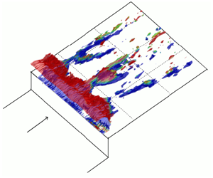
For the larger step heights, the initial growth and decay of  $U_{rms}^{\prime }$ near the wall appears to be related to the regions of reversed flow that occur shortly downstream of the step. Even though very little reversed flow is evident in the spanwise-averaged mean flow results, upon closer inspection, there are regions of reversed flow present for many of the cases studied. These regions become highly modulated by the stationary cross-flow vortices, which, in some cases, result in isolated regions of reversed flow. Since these regions are so isolated and weak, the spanwise-averaged velocity is positive. These reversed flow regions occur for all step heights at or above 1.5 mm, as well as for the 1.4 mm FFS with 4 layers of DREs. Figure 15 shows the regions of reversed flow as white contours, along with colour contours of the
  $U^{\prime }$-velocity at two different heights above the surface. The flow reversal in these cases is very weak, with maximum reversed flow velocities of less than 2 % to 3 %
  $U_{e}$. The regions of reversed flow extend approximately 7–15 mm downstream of the step, and are not very tall, typically less than 0.3 mm in height. It is interesting to note that the larger amplitude cross-flow vortices caused separation in this case (figure 15c), when separation was not measured for the same step height with lower stationary cross-flow amplitude (figure 15b). However, in both cases, regions of cross-flow reversal were measured. These cross-flow reversal regions are similarly modulated by the stationary cross-flow vortices.

Figure 15. Planform view of  $U$-disturbance velocity at
  $y=0.5~\text{mm}$. (a) 1.7 mm FFS. (b) 1.4 mm FFS. (c) 1.4 mm FFS with 4 layers of DREs. (d) 1.27 mm FFS. Black lines are inviscid streamline contours, and white lines are regions of flow reversal (
 $U_{\bot }\leqslant 0$) at
  $y=0.1~\text{mm}$.
Hosseinverdi & Fasel (Reference Hosseinverdi and Fasel2016) showed computationally that swept separation bubbles are highly destabilizing for stationary cross-flow instabilities, due to the inflectional nature of the profiles. They also showed that cross-flow reversal begins near the wall right before the beginning of separation, so these two phenomena are linked due to the adverse pressure gradient. In any case, either the cross-flow reversal results in a strong inflection point near the wall, or the flow reversal results in an inflection point. Thus, the observation made by Tufts et al. (Reference Tufts, Reed, Crawford, Duncan and Saric2017) that the helical flow region plays an important part in the amplification of the stationary cross-flow vortices is likely partially correct, however, there is no evidence to suggest that there is a constructive interaction between the helical flow region and the incoming vortices. In fact, given the highly localized nature of the helical flow regions, and the linear behaviour of the stationary cross-flow amplitude near the step, this explanation seems unlikely. Separation is simply a destabilizing influence on its own because of the inflectional and inviscidly unstable nature of the profiles and will cause stationary cross-flow growth regardless of the height of the centre of the incoming vortex. Naturally, as the strength and size of this region increases, due to increasing step height, the impact on the stationary cross-flow instabilities will increase as well. This is supported by the gradual increase in the initial growth rate of the stationary cross-flow instabilities that is observed as the step height is increased. There is no sudden critical behaviour, as one might expect if transition were to occur only when the incoming stationary cross-flow vortex were above a certain height.
We can further support this claim that the inflectional profiles near the step are primarily responsible for the strong stationary cross-flow growth by qualitatively comparing the behaviour of the stationary cross-flow vortices with those computed by Hosseinverdi & Fasel (Reference Hosseinverdi and Fasel2016). They showed that, upstream and downstream of the separation region, the isosurfaces of the  $U^{\prime }$-velocity follow the external streamlines, while, inside the separation bubble, they do not. Our results show a similar behaviour, particularly for the largest step height. Figure 15(a) shows that, near the step, the
  $U^{\prime }$-velocity contours bend outboard fairly aggressively before straightening out farther downstream, and aligning more closely with the external streamlines (black lines). An additional similarity is the abrupt phase shift that is seen in the
  $U^{\prime }$-contours shortly downstream of reattachment
  $(x-x_{s}\approx 15~\text{mm})$. This is particularly visible for the 1.7 mm FFS (figure 15a) and the 1.4 mm FFS with 4 layers of DREs (figure 15c). This behaviour was also observed by Hosseinverdi & Fasel (Reference Hosseinverdi and Fasel2016) (see figure 22), although they did not observe a second growth of the stationary cross-flow downstream of reattachment. Since their computations were linear, this would indicate that the second region of growth is a nonlinear effect, while the spatial phase shift is a linear effect, which appears to be related to reattachment. Also, notice at this point that there are some smaller wavelength harmonics starting to become visible at
  $y=0.5~\text{mm}$, particularly for the 1.7 mm FFS case, which further supports the nonlinear growth explanation.
There are also similarities between the measured stationary cross-flow mode shapes near the step, and those computed by Hosseinverdi & Fasel (Reference Hosseinverdi and Fasel2016). Depending on the stationary cross-flow wavelength, the disturbances exhibit double peaks, with the upper and lower peaks offset in phase by nearly  $180^{\circ }$. We see similar behaviour of our
  $U^{\prime }$-disturbance velocity contours, as shown in figure 16. These results are taken at two streamwise locations near the measured separated region for the 1.7 mm FFS case. Notice the upper
  $(y\approx 1.5~\text{mm})$ and lower
  $(y\approx 0.5~\text{mm})$ sets of
  $U^{\prime }$-disturbances that, at the second location, are offset by almost
  $180^{\circ }$. The phase shift between the two sets of disturbances increases as the flow progresses downstream, until eventually the two sets of disturbances appear to merge. Movies of the
  $U^{\prime }$-disturbance development downstream of the step for each case are included in the supplemental material available at https://doi.org/10.1017/jfm.2020.367. The numerous similarities between the current results and those of Hosseinverdi & Fasel (Reference Hosseinverdi and Fasel2016) indicate that the growth of the stationary cross-flow is simply the destabilizing result of the inflectional profiles introduced by the occurrence of a separation bubble.

Figure 16. The  $U^{\prime }$-disturbances downstream of the 1.7 mm FFS at (a)
  $x-x_{s}=10~\text{mm}$ and (b) 15 mm.
Since the second region of growth of the stationary cross-flow is believed to be a nonlinear phenomenon, it is beneficial to study the wavelength content of the stationary cross-flow instabilities and how this evolves downstream. Wavenumber spectra for the  $U^{\prime }$-velocity component are shown in figure 17 for all cases studied at a specific height in the boundary layer of
  $y=0.5~\text{mm}$. The spectra are shown only for the results that were acquired downstream of the step. In most cases (for step heights larger than 1.27 mm), at least some harmonics are visible downstream of the step, near where the amplitude of the primary wavelength
  $(\unicode[STIX]{x1D706}^{-1}\approx 0.1)$ begins to grow for the second time. For the 1.4 mm step with 4 layers of DREs, there are at least three harmonics visible even near the step, and they follow the same behaviour as the primary mode (growing, decaying and growing again). For the other cases, where the stationary cross-flow amplitude is not as large, the harmonics primarily appear only at or near the region where the second growth of the primary mode occurs, particularly the higher harmonics. In some cases the harmonics begin to become apparent upstream of the second growth region. These smaller wavelength modes appear to be affected differently by the near-step region and likely contribute to the nonlinear growth that occurs farther downstream.

Figure 17. Wavenumber spectra taken at  $y=0.5~\text{mm}$: (a) 1.27 mm FFS; (b) 1.4 mm FFS; (c) 1.4 mm FFS with 4 layers of DREs; (d) 1.5 mm FFS; (e) 1.6 mm FFS; (f) 1.7 mm FFS.
The flow reversal near the step is further studied by examining the vortices that are present near the step. This is accomplished by computing the swirling strength of the mean flow (Zhou et al. Reference Zhou, Adrian, Balachandar and Kendall1999; Tomkins & Adrian Reference Tomkins and Adrian2003; Wu & Christensen Reference Wu and Christensen2006; Chen et al. Reference Chen, Adrian, Zhong, Li and Wang2014). There are multiple methods for vortex extraction, but the swirling strength ( $\unicode[STIX]{x1D706}_{ci}$) criterion has been shown to perform well in flows where strong mean shear is present, such as in a boundary layer (Chen et al. Reference Chen, Li, Bai and Wang2018). The swirling strength is the imaginary part of the complex eigenvalues of the velocity gradient tensor. There is not a well-defined threshold for
  $\unicode[STIX]{x1D706}_{ci}$. On theoretical grounds, anything greater than zero should indicate the existence of a vortex, but, in practice, the results are too noisy. For the results presented here, a threshold of
  $\unicode[STIX]{x1D706}_{ci}=1$ is chosen. These results are illustrated in figure 18, which shows regions of reversed flow (
 $U_{\bot }\leqslant 0$) as red isosurfaces, along with isosurfaces of swirling strength (
 $\unicode[STIX]{x1D706}_{ci}$) in black, for three of the cases studied. The black isosurfaces are made to be somewhat transparent so that the reversed flow regions are still visible beneath them. The swirling strength identifies, for all cases, a spanwise-oriented vortex shortly downstream of the step. The spanwise vorticity near the step is very strong, due to both the strong negative streamwise gradient of the
  $V$ velocity (
 $\unicode[STIX]{x2202}V/\unicode[STIX]{x2202}x$), as well as the strong positive wall-normal gradient of the
  $U$ velocity (
 $\unicode[STIX]{x2202}U/\unicode[STIX]{x2202}y$). It is interesting, particularly for the two smaller step heights (figure 18b,c), that this vortex appears to exist continuously across the span, despite the strong modulation of, or complete lack of, reversed flow. In fact, this vortex was identified (by both swirling strength, and Q-criterion) to exist near the step for all step heights, including 1.27 mm and 1.4 mm, both of which had no regions of reversed flow. This region increases in length as the step height increases.
The main difference between the cases with and without reversed flow is that the cases with reversed flow result in modulation of the initial spanwise vortex. At a streamwise location close to the middle of the reversed flow regions, the swirling strength isosurfaces begin to show a strong modulation, with vortices identified in regions where the reversed flow is present. Finally, downstream of reattachment, several smaller streamwise-oriented vortices become apparent, typically located on either side of each separated region. Figure 19 shows a side view of these same isosurfaces for the 1.7 mm FFS. This figure illustrates the relative  $y$-locations of the recirculating regions, which occur very close to the wall, and the swirling strength isosurfaces, which occur above the recirculation.

Figure 18. Isosurfaces of swirling strength,  $\unicode[STIX]{x1D706}_{ci}=1$ (black) and reversed flow,
  $U_{\bot }\leqslant 0$, (red) for the (a) 1.7 mm FFS, (b) 1.4 mm FFS with 4 layers of DREs and (c) 1.27 mm FFS.

Figure 19. Side view of  $\unicode[STIX]{x1D706}_{ci}=1$ isosurfaces (black) and reversed flow (
 $U_{\bot }\leqslant 0$) isosurfaces (red) for the 1.7 mm FFS.

Figure 20. Isosurfaces of swirling strength,  $\unicode[STIX]{x1D706}_{ci}=1$, coloured by streamwise vorticity,
  $\unicode[STIX]{x1D714}_{x}$, for the 1.7 mm FFS.
In figure 20, isosurfaces of swirling strength are plotted for the 1.7 mm FFS case. This figure is zoomed in to show only three wavelengths of the stationary cross-flow. The isosurfaces are coloured by streamwise vorticity, which is computed as  $\unicode[STIX]{x1D714}_{x}=\unicode[STIX]{x2202}W/\unicode[STIX]{x2202}y-\unicode[STIX]{x2202}V/\unicode[STIX]{x2202}z^{\prime }$. The vorticity helps to clarify the rotation direction of the vortices that are identified by the swirling strength. The region nearest the step (A), as mentioned earlier, is oriented in the spanwise direction and dominated by positive spanwise vorticity (
 $\unicode[STIX]{x1D714}_{z}=\unicode[STIX]{x2202}U/\unicode[STIX]{x2202}y-\unicode[STIX]{x2202}V/\unicode[STIX]{x2202}x_{c}$), thus the contours of streamwise vorticity are not relevant until downstream of approximately 10 mm, where the isosurfaces become highly modulated. The vortices become modulated into smaller and smaller scales. Initially, there are larger regions identified by the swirling strength criterion (B) near
  $x-x_{s}=12~\text{mm}$, which look like smaller spanwise-oriented vortices that are breaking off from the upstream vortex. With these regions, it is difficult to determine exactly the rotation direction. There is always strong positive spanwise vorticity, due to the wall-normal velocity gradient of
  $U$ (
$U$ ( $\unicode[STIX]{x2202}U/\unicode[STIX]{x2202}y$). Given that there is also still flow reversal at this location, it is likely that these are still spanwise-rotating vortices. Farther downstream, as the flow reattaches, these regions become even more modulated into smaller streamwise-oriented vortices (C1–C3). In some cases (particularly the two wavelengths on the left in figure 20), there are three smaller vortices that become apparent. The one farthest to the left (C1) is rotating clockwise (positive
  $\unicode[STIX]{x1D714}_{x}$), while the other two (C2–C3) are rotating counterclockwise. The different rotation directions of these streamwise vortices are supported by the mean flow due to the modulated regions of cross-flow reversal. These streamwise vortices result from a deformation of the shear layer as the flow experiences the strong spanwise gradients caused by the stationary cross-flow vortices. In other words, the initially spanwise-oriented vortex is bent into a U-shape, due to the negative
  $\unicode[STIX]{x2202}U/\unicode[STIX]{x2202}z$ on the left side of the separation bubble, and the positive
  $\unicode[STIX]{x2202}U/\unicode[STIX]{x2202}z$ on the right side of the separation bubble. In addition, in most locations downstream of reattachment, the streamwise gradient of the
  $U$-velocity component is positive, meaning that there will be vortex stretching of the streamwise vortices, which would enhance the strength of these vortices. This behaviour provides a good explanation for the sudden appearance of the smaller wavelength harmonics downstream of reattachment. These smaller wavelength scales are introduced by the modulation of the separation bubble, resulting in multiple streamwise-oriented vortices for each of the isolated separated regions. This further supports the conjecture that the second region of growth of the stationary cross-flow, which begins near reattachment, is a nonlinear effect. It is clear that the strong modulation of the reversed flow regions, which increases with increasing stationary cross-flow amplitude, results in the appearance of multiple, highly localized, streamwise vortices.

Figure 21. Plot of  $U$-velocity versus
  $x-x_{s}$ downstream of the 1.7 mm FFS. Results are at
  $y=0.5~\text{mm}$, and two spanwise locations.
The mechanism through which vortex shedding occurs from separation bubbles has been identified by Boghosian & Cassel (Reference Boghosian and Cassel2016) as occurring when the streamwise pressure gradient signature is such that there is an adverse pressure gradient upstream, followed by a favourable pressure gradient downstream. This essentially results in a tearing apart of the shear layer. Although the results shown in figure 20 are computed based off of the mean flow, and, therefore, are not showing an instantaneous vortex-shedding event, this mechanism still may provide an explanation for the behaviour that occurs in the mean flow, where the smaller spanwise-oriented vortices (B) tear off from the initial spanwise vortex (A). Tufts et al. (Reference Tufts, Reed, Crawford, Duncan and Saric2017) showed that, when a forward-facing step is encountered, there is an initial adverse pressure gradient upstream of the step, followed by a very short region of favourable pressure gradient at the step, followed by another region of adverse pressure gradient. Since there is an imposed favourable pressure gradient, this adverse pressure gradient region will eventually relax back to this imposed favourable gradient (i.e. the baseline condition). Thus, downstream of the step, the flow does encounter the specific pressure gradient signature (adverse followed by favourable) required for this vortex-shedding mechanism. In addition, the gradients become more severe within the boundary layer in regions where separation is encountered. This is illustrated in figure 21, which shows the  $U$-velocity at
  $y=0.5~\text{mm}$ versus
  $x-x_{s}$ at two different spanwise locations. One of the spanwise locations,
  $z=15~\text{mm}$, is near the middle of one of the separated regions, while the other,
  $z=8~\text{mm}$, is outside of any separated region. It is clear from this figure that, when a separation bubble is encountered, the streamwise velocity gradients (and, therefore, pressure gradients) within the boundary layer are much stronger, both upstream and downstream of the bubble. This could explain the modulation and tearing of the vortices that was observed to occur in figure 18(a,b). In addition, the gradient direction changes from adverse (negative slope of
  $U$) to favourable (positive slope) shortly downstream of
  $x-x_{s}=10~\text{mm}$, which is exactly where the modulation of the initial vortex begins in the regions of reversed flow (figures 18a and 20).
4.5 Effect of steps on unsteady disturbances

Figure 22. Planform view of  $u_{rms}^{\prime }$ velocity at
  $y=0.5~\text{mm}$ for the (a) 1.7 mm FFS, (b) 1.6 mm FFS, (c) 1.52 mm FFS and (d) 1.4 mm FFS with 4 layers of DREs. Black contour lines indicate regions of reversed flow near the wall (
 $U_{\bot }\leqslant 0$).
The unsteady mechanisms that lead to breakdown downstream of the steps will be discussed in this section. The fluctuating velocity ( $u_{rms}^{\prime }$) contours at
  $y=0.5~\text{mm}$ are shown in figure 22 for the three largest step heights, and for the 1.4 mm FFS case with 4 layers of DREs. The other cases did not exhibit any substantial
  $u_{rms}^{\prime }$ growth, so they are not included in this figure. These figures also include black contour lines indicating regions of reversed flow near the wall
  $(y\approx 0.1~\text{mm})$. For the 1.52 mm FFS height (figure 22c), a
  $u_{rms}^{\prime }$ disturbance begins to become apparent toward the inboard side of the measurement area starting at approximately 25 mm downstream of the step. The
  $u_{rms}^{\prime }$ disturbance appears progressively closer to the step as the step height is increased, and the amplitudes reach larger values. For the 1.6 and 1.7 mm FFS cases, the amplitudes of
  $u_{rms}^{\prime }$ begin to grow significantly starting at approximately 15–20 mm downstream of the step. However, the disturbances are present starting shortly downstream of the step. For the 1.4 mm FFS case with four layers of DREs (figure 22d), the
  $u_{rms}^{\prime }$ disturbance is already quite large immediately downstream of the step. It appears to decay for a short distance before it grows again significantly at 15 mm downstream of the step, near the reattachment location. From these figures, the locations of the fluctuations appear to be closely related to the regions of reversed flow. For the 1.6 and 1.7 mm FFS (figure 22a,b), the large growth in amplitude of the fluctuations begins abruptly near reattachment, particularly between
  $z=-10$ and 10 mm. At other locations, there are smaller regions of increased fluctuation amplitude emanating from the centre of the separation bubble after reattachment, and these eventually (about 10 mm farther downstream) begin to spread in the spanwise direction. In some cases there are very small lines of increased fluctuation evident on either side of the separation bubbles, or there are multiple smaller lines beginning after reattachment and continuing downstream. These results make sense in light of the vortex identification that was performed in the previous section. This analysis identified the presence of multiple small-scale vortices in the mean flow that are produced as a result of the modulation of the separated regions. Given the unsteady and unstable nature of separation bubbles, it is likely that these fluctuations that occur downstream of reattachment are due to vortices that are shed from the separation bubble. It is interesting that even the tiniest of separation bubbles, such as those present in the 1.4 mm FFS case with 4 layers of DREs, result in such large fluctuations downstream of reattachment (figure 22d). In this case, there are thin bands of fluctuations present along both sides of the separation bubble.
The vortex-shedding mechanism identified by Boghosian & Cassel (Reference Boghosian and Cassel2016) as occurring when the streamwise pressure gradient signature is such that there is an adverse pressure gradient upstream, followed by a favourable pressure gradient downstream, could also result in unsteady vortex shedding near reattachment. This pressure gradient signature, while already present in the mean flow, can also be enhanced at certain times due to fluctuations of the shear layer. These fluctuations can occur due to different mechanisms, the most prevalent of which are unsteady instabilities in the shear layer (such as the Kelvin–Helmholtz instability). This pressure gradient profile occurs at a certain point in the phase of the unsteady instabilities that are perturbing the shear layer, and causes the shear layer to tear itself apart and shed a vortex downstream. Thus, the unsteadiness that occurs in or near the shear layer ultimately leads to the shedding of vortices near reattachment, which leads to breakdown. The initial unsteadiness of the shear layer could be caused by different mechanisms, such as a flapping of the shear layer, Kelvin–Helmholtz instabilities, or even high-frequency secondary instabilities. High-frequency secondary instabilities, which typically lead to breakdown in stationary cross-flow dominated flows, occur in regions of strong wall-normal or spanwise shear caused by the stationary cross-flow vortices. There are regions of strong spanwise and wall-normal shear present, even though the mean flow (see line contours of figure 24) does not resemble the highly inflectional profiles that typically occur when these fluctuations are measured (such as that seen by White & Saric (Reference White and Saric2005) or Malik et al. (Reference Malik, Li, Choudhari and Chang1999)).
Time-resolved PIV results were acquired at 8 kHz for several select conditions and locations to try to learn more about the nature of these fluctuations. The TRPIV results reveal a high-frequency instability beginning shortly downstream of the step for the critical step heights. The peak frequency occurs between 0.5 and 2 kHz, depending on the step height and location, as shown in figure 23. This figure shows the spanwise-averaged spectra at various streamwise locations for the same step heights presented in the previous two figures. This frequency range is approximately that of the high-frequency secondary instabilities seen in the baseline (no step) case (Eppink et al. Reference Eppink, Wlezien, King and Choudhari2018). As the flow progresses farther downstream, the spectra begin to broaden, and there is some lower frequency content that becomes more prominent, in the 200–700 Hz range. The 1.5 mm FFS case did not exhibit any strong fluctuations near the step, so the high-speed measurements are shown starting farther downstream. In general, the peak frequency of the fluctuations seems to increase as the step height is increased. The exception is the 1.4 mm FFS with 4 layers of DRES. This case exhibits a higher-frequency peak than any of the other cases, at  $f=2500~\text{Hz}$.

Figure 23. Velocity spectra acquired at  $y=0.6~\text{mm}$ and several streamwise locations for the (a) 1.7 mm FFS, (b) 1.6 mm FFS, (c) 1.52 mm FFS and (d) 1.4 mm FFS with 4 layers of DREs.

Figure 24. The  $u_{rms}^{\prime }$ contours (colours) with black contour lines of mean streamwise (
 $U$) velocity, and red contour lines of reversed flow (
 $U_{\bot }\leqslant 0$). Results shown at (a, b)
  $x-x_{s}=10~\text{mm}$ and (c,d)
  $x-x_{s}=20~\text{mm}$. In (a,c) the
  $u_{rms}^{\prime }$ contours are integrated from
  $f=200$ to 700 Hz, and in (b,d) the
  $u_{rms}^{\prime }$ contours are integrated from
  $f=900$ to 2500 Hz.
Several studies have found that the vortex-shedding frequency of separated shear layers occurs in the range of 0.6–0.7  $U_{e}/l_{sb}$, where
  $l_{sb}$ is the time-averaged length of the separation bubble (Kiya & Sasaki Reference Kiya and Sasaki1983, Reference Kiya and Sasaki1985; Cherry, Hillier & Latour Reference Cherry, Hillier and Latour1984). The same studies also found that the low-frequency flapping occurs in the range of 0.12–0.2
  $U_{e}/l_{sb}$. Since these studies were performed in two-dimensional flows, it is not clear how well exactly they will correspond to a highly three-dimensional flow. However, the frequency ranges are expected to be somewhat similar. For the present measurements, the separation bubble length ranges from approximately 7–15 mm. Using the criteria of 0.6–0.7
  $U_{e}/l_{sb}$, this gives a frequency range of approximately 900–2300 Hz. These values are in good agreement with the higher-frequency peaks that are observed. Using the lower-frequency criteria of 0.12–0.2
  $U_{e}/l_{sb}$, we obtain a frequency range of approximately 190–650 Hz. This frequency range agrees very well with the lower frequencies that become more prevalent starting near the end of the separation bubble, which would imply that these fluctuations may be related to a flapping of the shear layer.
Contours of  $u_{rms}^{\prime }$ amplitude are shown for two different locations downstream of the 1.6 mm FFS in figure 24. The
  $u^{\prime }$-spectra were integrated over the two frequency ranges identified above (200–700 Hz, and 900–2500 Hz) in order to examine any differences that may exist. Additionally, contours of the time-averaged
  $U$-velocity are shown in black, and contours of reversed flow (
 $U_{\bot }\leqslant 0$) are shown in red. The first station shown was taken near the end of the separation bubble, so some small regions of recirculation are visible, while there is no reversed flow at the second location.
Figure 25 includes these same  $u_{rms}^{\prime }$ colour contours at
  $x-x_{s}=10~\text{mm}$, along with line contours of the largest wall-normal shear (
 $\unicode[STIX]{x2202}U/\unicode[STIX]{x2202}y$) and spanwise shear (
 $\unicode[STIX]{x2202}U/\unicode[STIX]{x2202}z$) values measured. These plots also contain a black contour line that indicates the location of the shear layer, located by plotting points of null curvature (where
  $\unicode[STIX]{x2202}^{2}U/\unicode[STIX]{x2202}z^{2}+\unicode[STIX]{x2202}^{2}U/\unicode[STIX]{x2202}y^{2}=0$). The higher frequency fluctuations tend to occur along the shear layer, in the regions of large wall-normal shear. On the other hand, the lower frequency fluctuations, particularly on the right side of the figure, seem to align more with the regions of large positive and negative spanwise shear (figure 25c). Similar results are shown at
  $x-x_{s}=20~\text{mm}$ in figure 26. Some regions of higher amplitude fluctuations still occur along the shear layer, while still others align more with regions of high spanwise shear, particularly for the higher-frequency fluctuations. In general, these fluctuations no longer occur primarily in the regions of largest wall-normal shear (indicated by the red contours). At this location, the highest fluctuation levels within both frequency ranges are primarily concentrated within the regions of largest negative spanwise shear (indicated by the blue contours in figure 26c,d).

Figure 25. The  $u_{rms}^{\prime }$ contours (colours) at
  $x-x_{s}=10~\text{mm}$ along with contours of (a,b) wall-normal shear (
 $\unicode[STIX]{x2202}U/\unicode[STIX]{x2202}y$) and (c,d) spanwise shear (
 $\unicode[STIX]{x2202}U/\unicode[STIX]{x2202}z$). The contours of shear are red and blue indicating positive and negative values, respectively. The black contour line shows the location of the shear layer, indicated by points of null curvature
  $(\unicode[STIX]{x2202}^{2}U/\unicode[STIX]{x2202}z^{2}+\unicode[STIX]{x2202}^{2}U/\unicode[STIX]{x2202}y^{2}=0)$. In (a,c) the
  $u_{rms}^{\prime }$ contours are integrated from
  $f=200$ to 800 Hz, and in (b,d) the
  $u_{rms}^{\prime }$ contours are integrated from
  $f=900$ to 2500 Hz.

Figure 26. The  $u_{rms}^{\prime }$ contours (colours) at
  $x-x_{s}=20~\text{mm}$ along with contours of (a,b) wall-normal shear (
 $\unicode[STIX]{x2202}U/\unicode[STIX]{x2202}y$) and (c,d) spanwise shear (
 $\unicode[STIX]{x2202}U/\unicode[STIX]{x2202}z$). The contours of shear are red and blue indicating positive and negative values, respectively. The black contour line shows the location of the shear layer, indicated by points of null curvature
  $(\unicode[STIX]{x2202}^{2}U/\unicode[STIX]{x2202}z^{2}+\unicode[STIX]{x2202}^{2}U/\unicode[STIX]{x2202}y^{2}=0)$. In (a,c) the
  $u_{rms}^{\prime }$ contours are integrated from
  $f=200$ to 800 Hz, and in (b,d) the
  $u_{rms}^{\prime }$ contours are integrated from
  $f=900$ to 2500 Hz.
These results provide important information about the origin of the fluctuations that lead to vortex shedding near reattachment. Since the higher-frequency fluctuations within the separated regions align very well with the shear layer, these instabilities are believed to be due to a Kelvin–Helmholtz type of instability. The lower frequency fluctuations, on the other hand, tend to occur along the left and right edges of the distorted shear layer. These frequencies fall within the range of expected flapping frequencies of the shear layer. These fluctuations may be a result of a spanwise expansion and shrinking motion of the three-dimensional shear layer, due to a flapping or breathing mechanism. As mentioned, these fluctuations also occur in regions of larger spanwise shear, so it is worth considering that they are associated with a secondary instability of the stationary cross-flow. However, the frequencies are lower than expected for this instability, which was found to be near 2 kHz in the absence of the step. Additionally, secondary instabilities typically only occur in regions of strong negative spanwise shear, whereas, these fluctuations, within the separated regions, are seen in regions of both positive and negative spanwise shear. Thus, these seem unlikely to be related to a secondary instability mechanism. Downstream of reattachment, the fluctuations within both frequency ranges align more with the regions of larger negative spanwise shear, so there may be some high-frequency secondary instabilities occurring downstream of reattachment. However, the sudden increase in fluctuation amplitude downstream of reattachment is best explained by a vortex-shedding mechanism, as discussed previously, since this location is not associated with a sudden increase in spanwise shear. In fact, as shown in figure 14(a), the downstream location  $(x-x_{s}=20~\text{mm})$ is associated with a local minimum in the amplitude of the stationary cross-flow vortices.
5 Conclusions
The mechanisms through which a swept forward-facing step modifies the growth of the stationary cross-flow instability and leads to transition have been studied and identified as follows. The initial stationary cross-flow growth near the step is linked to the strong inflection points that occur shortly downstream of the step through the introduction of reversed flow and cross-flow reversal. Both of these phenomena occur because of the adverse pressure gradient induced by the step. There is no evidence to support the previously reported conjecture that the incoming stationary cross-flow vortices interact constructively with the reversed flow region. In fact, many similarities were found between the current measurements and linear computations of stationary cross-flow interactions with a separation bubble on a swept wing, indicating that the initial growth is a linear phenomenon, and simply due to the destabilizing influence of the inflectional profiles.
In contrast, the second region of growth of the stationary cross-flow vortices is linked to nonlinear effects. The strong stationary cross-flow vortices near the step cause a spanwise deformation of the shear layer, which ultimately results in the formation of multiple, small, streamwise-oriented vortices within each wavelength of the primary mode. Thus, harmonics of the primary mode are suddenly triggered within the boundary layer near the reattachment location, leading to a region of nonlinear growth. The initial modulation of the reversed flow regions depends on the initial stationary cross-flow amplitude. The more modulated these regions become, the stronger this mechanism becomes.
Finally, the localized unsteady fluctuations measured downstream of reattachment, which ultimately cause transition, are linked to vortices that shed from the distorted shear layer. This mechanism explains the sudden growth in fluctuation amplitude that occurs, in most cases, shortly downstream of reattachment. The initial mechanism that causes unsteadiness of the shear layer is not definitively identified, but evidence points to a shear-layer instability as the primary culprit.
It was shown that the initial stationary cross-flow amplitude is an important factor in this process due to its effect on the modulation of the shear layer, leading to downstream growth of the stationary cross-flow, as well as unstable shear layers that lead to, in some cases, large amplitude fluctuations. Note that all of these measurements were performed with some level of forcing of the stationary cross-flow. While no detailed measurements were performed for cases with no DREs, flow-visualization results indicate that the transition mechanisms are similar. As would be expected, since the stationary cross-flow amplitudes are lower, the critical step heights with no forcing tended to be slightly larger than with forcing. However, the transition front was much less uniform, which led to the decision to use forcing. Of course, on a real aircraft wing, DREs will not be present. However, there will always be some level of roughness on any real surface. Additionally, on transport aircraft, the boundary layer will be very thin, and thus, sensitive to very small levels of surface roughness. Thus, stationary cross-flow will likely be present, to some degree. The amplitude will also depend on the streamwise location of the step. Given the important role of the stationary cross-flow amplitude in the transition process over a forward-facing step, it is important to keep these effects in mind when developing transition criteria and manufacturing tolerances for swept wings. Another point that should be discussed is the possible influence of the free-stream fluctuations on transition in this scenario. It is well known that shear layers can be quite sensitive to free-stream acoustic fluctuations. It is possible in these cases, due to the three-dimensionality of the separation bubbles, that the shear layers are also sensitive to vortical fluctuations in the free stream. Thus, the behaviour in flight may be different than that observed in the wind tunnel, since the fluctuation levels are expected to be significantly lower in flight. It would be interesting and beneficial to determine whether this transition mechanism is consistent between multiple wind tunnel facilities and in flight.
Declaration of interests
The authors report no conflict of interest.
Supplementary material
Supplementary material is available at https://doi.org/10.1017/jfm.2020.367.


