


I. INTRODUCTION
The properties of polycrystalline materials are determined by the properties of each crystallite and the boundaries between crystallites. The size of the crystallites in a polycrystalline material has significant effects on many of its properties, such as thermal, mechanical, electrical, magnetic, and chemical properties. For instance, the mechanical strength of polycrystalline metals and alloys are strongly dependent on the crystallite (grain) size. In many applications, it is very important to know not only the average crystallite size but also crystallite size distribution (CSD). Recently, crystal/particle size analysis on pharmaceutical materials has gained more interest since the crystallite size determines many characteristics of drug substance. For instance, in the pharmaceutical industry, the crystallite size and size distribution are important parameters for process control in drug research, production, and the properties of the final products, such as the stability, solubility, permeability, and dissolution on oral drug absorption. Depending on the field of applications, grain size or particle size may be referred to in place of crystallite size. A grain or a particle can be either a single crystal or an agglomeration of several crystallites. The method described in this paper may also be used to determine grain size distribution or particle size distribution as long as each grain or particle are single crystal.
X-ray diffraction has been used for crystallites size measurement for over 90 years since Scherrer (Reference Scherrer1918) and subsequent contribution were made by Stokes and Wilson (Reference Stokes and Wilson1942) and Warren and Averbach (Reference Warren and Averbach1952). All these methods are based on diffraction line broadening and line profile analysis as summarized by Leoni (Reference Leoni, Gilmore, Kaduk and Schenk2019). With a sample containing large grain size or when a small incident beam is used, spotty diffraction rings are observed in a 2D diffraction pattern (Cullity, Reference Cullity1978). Many approaches are suggested to measure crystal size and size distribution (Hirsch, Reference Hirsch1952a, Reference Hirsch1952b; Hirsch and Kellar, Reference Hirsch and Kellar1952; Rodriguez-Navarro et al., Reference Rodriguez-Navarro, Alvarez-Lloret, Ortega-Huertas and Rodriguez-Gallego2006; Neher et al., Reference Neher, Klein and Kuhs2019). Crystallite size analysis from the γ-profile analysis of spotty 2D diffraction patterns is proposed by He (Reference He2009, Reference He2014). The γ-profile analysis has been used to measure the grain size of planetary materials (Bramble et al., Reference Bramble, Flemming and McCausland2015) and particle size in drug tablets (Thakral et al., Reference Thakral, Thakral and Suryanarayanan2017).
The crystallite size analysis from FWHM of 2θ peaks by Scherrer equation is limited to crystallite size below 100 nm, while γ-profile analysis is a complementary method which can extend the crystallite size measurement range up to a few millimeters by proper instrumentation and data collection strategy (He, Reference He, Gilmore, Kaduk and Schenk2019). However, either the Scherrer equation or the γ-profile method can only measure the average crystal/particle size, but not the size distribution.
In this paper, a method to measure crystallite size distribution by two-dimensional X-ray diffraction is proposed. First, diffraction spots within a particular diffraction ring are identified by image recognition. The intensity of a diffraction spot is determined by both the crystallite size and orientation. In order to measure the intensity of a diffraction spot solely related to the corresponding crystallite size, multiple frames are collected at various rocking angles. The rocking curves can be constructed from the multiple frames for all measured diffraction spots. The maximum intensity of each spot can be determined, and which is proportional to the volume of corresponding crystallites. Then crystallite size distribution can be evaluated from one rocking scans or sum of multiple scans.
II. CRYSTALLITE SIZE MEASURED BY γ-PROFILE ANALYSIS
Two-dimensional X-ray Diffraction (XRD2) pattern from a polycrystalline or powder sample with fine crystallite size (also referred to as grain size or particle size in some articles) shows a smooth diffraction ring, while the XRD2 pattern from a sample with larger crystallites or collected with a small beam size shows spotty diffraction rings. The crystallite size can be measured by the spottiness of the diffraction ring by γ-profile analysis.
Figure 1 shows a frame collected from a SRM660a (LaB6) sample with an XRD2 system (GADDS™) in transmission mode and with CuKα X-rays. The beam size b is approximately 200 μm produced by a double pinhole collimator. The detailed specifications of the optics can be found in the section 3.3.7 of He (Reference He2009). The sample thickness t is 7.0 μm. With a 23.75 cm sample-to-detector distance, three rings from (100), (110), and (111) planes are observed on this frame. The γ-profile of (110) line, produced by 2θ-integration over a defined 2θ and γ range, is displayed in the bottom of the figure. The number of crystallites contributing to the diffraction pattern within the integrated region can be estimated from the number of intersections of the γ-profile with a threshold line. Every two intersections of γ-profile with this threshold line represents a crystallite. In this case, the 2nd order polynomial trend line of the γ-profile intensities is used as the threshold line.

Figure 1. The diffraction pattern for SRM660a (LaB6) and the corresponding γ-profile that can be used for crystallite size analysis.
The detailed theoretical analysis can be found in He (Reference He2018), but the theory can be simply explained by a “candy box”. The effective diffraction volume, also referred to as gauge volume, can be considered as a candy box. As the number of candies to fill the box depends on the size of the candy and box, the number of spots along the diffraction ring in a given γ range is also associated with the crystallite size. Based on the effective diffraction volume and the crystallographic nature and crystallite size of the sample, the equation for crystallite size measured in reflection mode is given as:
 $$d = \left\{{\displaystyle{{3{\boldsymbol p}_{{\boldsymbol hkl}}A_0\beta \arcsin [ \cos \theta \sin ( \Delta \gamma /2) ] } \over {2\pi^2\mu N_s}}} \right\}^{1/3}$$
where d is the average diameter of the crystallite particles, phkl is the multiplicity of the diffracting planes, A 0 is the cross-section of the incident X-ray beam, β is the divergence of the incident X-ray beam, μ is the linear absorption coefficient, and Ns is the number of crystallites contributing to the diffraction pattern. The Δγ is the measured range of the diffraction ring. As an example, the Δγ of (110) ring in Figure 1 is 46° (from γ = −67° to γ = −113°). Introducing a scaling factor covering all the numeric constants, incident beam divergence and calibration factor for the instrument, we obtained an equation for the crystallite size measurement in reflection mode
 $$d = k\left\{{\displaystyle{{{\boldsymbol p}_{hkl}{\boldsymbol b}^2\arcsin [ \cos \theta \sin ( \Delta \gamma /2) ] } \over {2\mu N_s}}} \right\}^{1/3}$$
where b is the size of the incident beam and k = (3β/4π)1/3 is the instrumental broadening in 2θ direction. But we may treat k as a calibration factor which can be determined from the 2D diffraction pattern of a standard sample with known crystallite size. Since only a limited number of spots along the diffraction ring can be resolved, it can be seen from the equation that a smaller X-ray beam size and low multiplicity peak should be used if a smaller crystallite size is to be determined.
For measurement in transmission mode with a sample thickness of t, we have:
 $$d = k\left\{{\displaystyle{{{\boldsymbol p}_{{hkl}_i} b^2{\boldsymbol t}\arcsin [ \cos \theta \sin ( \Delta \gamma /2) ] } \over {N_s}}} \right\}^{1/3}$$
The effective sampling volume reaches a maximum for transmission mode diffraction when t = 1/μ. It can be observed from the above equations that the effective sampling volume is proportional to the beam cross-section area and is lower for materials with higher linear absorption coefficients. The sample absorption has a different effect on the sampling volume in reflection and transmission modes. In reflection mode, the linear absorption coefficient determines how fast the incident beam is attenuated within the sample, but there is no clear cutoff for the penetration depth. Therefore, the effective sampling volume has to be used. In transmission mode with the incident beam perpendicular to the sample surface, the linear absorption coefficient affects the relative scattering intensity, but not the actual sampling volume. In other words, all the sample volume within the beam path contributes to the diffraction. Therefore, it is reasonable to ignore the absorption effect for crystallite size analysis as long as the sample is thin enough for transmission mode diffraction.
The incident X-ray beam size should be determined by the crystallite size. In cases where too few diffraction spots can be observed in the diffraction ring, a large beam size or sample oscillation (by rotation or translation) may improve the sampling statistics. For the sample with very large crystallite size relative to the beam size, the number of the spots on the diffraction ring may be too few to have a reliable count. In this case, the effective volume can be increased to cover more crystallites by scanning the X-ray beam over certain area of the sample or collecting the diffraction frame at multiple targets on the sample. In the multiple target method, one diffraction frame is collected by accumulating the data collection at multiple targets. Alternatively, multiple frames can be collected at one frame on each target, and then add all frames into one frame. All the above quoted measures, including rotation and/or translation during data collection, multiple targets, and multiple frames, have a single purpose, that is to increase the number crystallites to be counted (increase the instrument window), so a crystallite size based on the average volume of crystallites can be calculated from γ-profiles with a better statistics. However, the crystallite size distribution information cannot be obtained by the γ-profile method.
III. CRYSTALLITE SIZE AND SIZE DISTRIBUTION
In order to measure the crystallite size distribution, the size or volume of each and all crystallites covered by the set instrument window should be measured. Thus, each and all diffraction spots at various rocking angles need to be identified and traced. So that the diffraction intensities only relevant to the crystallite size are obtained.
A. Rocking curve with a 0D detector
In Figure 2 (left), the incident X-rays hit the crystal planes with an incident angle θ and reflection angle θ. The diffraction peak is observed when the Bragg condition is satisfied:
 $$2d_{hkl}{\rm sin}\theta = \lambda $$
where λ is the wavelength, dhkl is the distance between each adjacent (hkl) crystalline planes (d-spacing), θ is the Bragg angle at which one observes a diffraction peak. The vector s0/λ represents the incident X-ray beam and the vector s/λ represents the scattered beam. N(hkl) is the normal of the crystalline plane (hkl). When the Bragg condition is satisfied the diffraction vector Hhkl is perpendicular to the crystal planes and the three vectors have the following relationship:
 $$\displaystyle{{{\boldsymbol s}-{\boldsymbol s}_0} \over \lambda } = {\boldsymbol H}_{hkl}$$
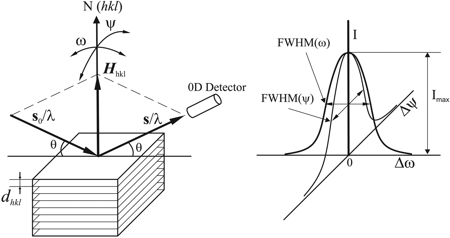
Figure 2. (left) Bragg condition and crystal rocking. (right) Rocking curve in both rocking directions.
The intensity of the diffraction is given by the total counts or photons collected by the 0D detector and denoted by I. At the above perfect Bragg condition, the intensity is given as Imax. The normal of the crystal plane N(hkl) can be rotated (rocking) away from the orientation of the diffraction vector Hhkl by either ω rotation or ψ rotation in a typical X-ray diffractometer. When the crystal plane normal rotates (rocking) away from the orientation of the diffraction vector Hhkl, the diffraction intensity collected by the 0D detector may not drop to zero immediately, but gradually as a function of the rocking angles Δω or Δψ. The rocking angles Δω or Δψ are defined as the angular deviation from perfect Bragg condition. The diffraction intensity as a function of the rocking angle Δω or Δψ are plotted in the right of Figure 2. The relationship between the diffraction intensity I and the rocking angle Δω or Δψ is called as rocking curve. Both rocking curves can be referred to as rocking curve (ω-scan) or rocking curve (ψ-scan) respectively, or simply ω-rocking curve and ψ-rocking curve. The full width at the half maximum of the rocking curve in both rocking direction is given as FWHM(Δω) and FWHM(Δψ). The FWHM and the profile of the rocking curve are determined by the defects of the crystal (such as mosaicity) and instrument condition (such as beam divergence).
B. Rocking curve with a 2D detector
Figure 3 illustrates the geometry for rocking curve collection with a 2D detector. If the sample is a fine powder or polycrystalline materials, a diffraction ring would be collected as shown in the image. For a single crystal at Bragg condition, spot P represents the location where the scattered X-ray beam (s/λ) hits the detection plane. The spot R along the trace of diffraction ring represents a scattered X-ray beam (s′/λ) deviated from (s/λ). The deviation in the 2D image is given by Δγ. The γ angle is used to define a location along the diffraction ring (He, Reference He2018). Correspondingly, the diffraction vector  ${\boldsymbol {H}^{\prime}}_{_{hkl} }$ is deviated from the direction of Hhkl by an angle of Δψ. This deviation is equivalent to rocking the crystal sample by ψ rotation. The equivalent rocking angle is given as
 $${\rm \Delta }\psi = 2{\rm arcsin}\left[{{\rm cos}\theta \sin \left({\displaystyle{{{\rm \Delta }\gamma } \over 2}} \right)} \right]$$
Figure 3. Rocking curve with a 2D detector.
Therefore, a virtual ψ-rocking curve can be obtained from the intensity distribution along the trace of diffraction ring, without actual ψ rotation of the sample. The ω-rocking curve can be collected in the same way as 0D detector by ω scan. The combination of the virtual ψ-rocking coverage and ω-rocking scan can ensure that the intensity at the perfect Bragg condition (Imax) to be measured.
C. Diffraction spots on 2D image
In the γ-profile analysis, the number of contributing crystallites for a measured diffraction ring (N s) is evaluated from γ-profile produced by 2θ integration. This method assumes all spots on a selected diffraction ring have the same 2θ, in another word, the diffraction spots are distributed along the diffraction ring. But in reality, crystallites are oriented in all possible directions, the diffracting crystallites are oriented either in perfect Bragg condition or within a vicinity of the Bragg condition. Therefore, some diffraction spots are aligned exactly on a constant 2θ ring, some are scattered around the diffraction ring. Figure 4 shows a diffraction frame collected from a proprietary multilayer battery anode with a Bruker VÅNTEC-500 2D detector. It shows that not all diffraction spots are aligned along a constant 2θ ring. Some spots can be separated from other spots only because of different 2θ values as shown in the two magnified boxes. These spots can be distinguished on the 2D frame, but may be merged in the γ-profile, resulting in inaccurate spots count. Apparently, the number of contributing crystallites for a measured diffraction ring (N s) can be more accurately counted directly on the 2D frame.

Figure 4. A 2D diffraction pattern for a proprietary multilayer battery anode with large crystallite size showing many spots varying from a constant 2θ ring.
There are many software packages available to identify the peaks/spots. For example, many single-crystal diffraction software packages have peak finding routines to evaluate the spots in 2D diffraction patterns (Schlichting, Reference Schlichting2015; Hadian-Jazi et al., Reference Hadian-Jazi, Sadri, Barty, Yefanov, Galchenkova, Oberthuer, Komadina, Brehm, Kirkwood, Mills, de Wijn, Letrun, Kloos, Vakili, Gelisio, Darmanin, Mancuso, Chapmand and Abbey2021). Peak/spot finding may involve user-selected threshold for determining a peak above the background or separation of merging spots. A similar software can be developed to identify spots along a diffraction ring.
Once the number of diffraction spots Ns is determined by peak finding software on the selected region defined by 2θ 1, 2θ 2, γ 1, γ 2 values. The average crystallite size can be calculated with Eq. (2) or Eq. (3) depending on the diffraction mode.
D. Diffraction intensity and crystallite size
In the crystallite size measurement by γ-profile method given in Section II, we assume that all crystallites are the same size. Or the measured crystallite size represents an average value. In many cases, it is necessary to measure the crystallite size distribution. The diffraction intensity of each spot is determined by at least two factors, one is the crystallite size and the other is the crystallite orientation relative to the diffraction vector. Figure 5 shows the integrated diffraction intensity determined by crystallite size and orientation. Assuming that the sample is single phase powder or polycrystalline, the incident X-ray beam has a cross-section size large enough to fully cover the crystallites A, B, and C, three diffraction spots are produced respectively on the trace of diffraction ring. The intensity of each diffraction spot is given by the total X-ray counts within the area of the spot. The crystallite A and B are so oriented that perfect Bragg condition is met. In another word, the intensity is given by the maximum intensity of the rocking curve. Due to the different crystallite size, the intensity from A and B are different. Without considering the effect of absorption and extinction, the intensity is proportional to the volume of the crystallite. Therefore, the size of the crystallites A and B can be evaluated from the respect intensity I A and I B. The orientation of crystallite C cannot fully satisfy the Bragg condition within the instrument window, so that diffraction intensity is not proportional to the size of the crystallite. The intensity I C is given by the intensity away from the maximum of the rocking curve. Due to the above reason, crystallite size distribution cannot be determined simply by the peak intensities on the γ-profile or intensity variation of diffraction spots on a single 2D frame.

Figure 5. The intensity of a diffraction spot as a function of crystallite size and orientation.
E. Maximum spot intensity from the rocking curve
In order to evaluate the crystallite size distribution, the intensity of each crystallite should be measured at the peak of rocking curve, Imax. With a two-dimensional detector, the rocking curve in ψ direction is covered by the γ angular range, therefore, ω scan is sufficient to reach the peak of the rocking curve. Figure 6 shows the rocking scan at reflection mode and transmission mode. In reflection mode, the sample is so thick that only scattered X-ray by reflection is considered. In a typical configuration at neutral position, the sample surface normal n bisects the incident and scattered X-rays. The rocking scan is achieved by rotating the sample in ω direction so the surface normal n scans over a ω range in the vicinity of the neutral position.

Figure 6. Rocking scan in reflection mode and transmission mode.
In transmission mode, the sample has a limited thickness t which allows the X-rays pass through. In a typical configuration at neutral position, the incident X-ray is perpendicular to the sample surface. In another word, the sample normal n is in the same direction as the incident beam. The rocking scan is achieved by rotating the sample in ω direction so the surface normal n scans over an angular range relative to the incident beam direction.
The transmission mode is preferred for crystallite size distribution measurement because the results are less affected by the sample absorption. The rocking scan can also be achieved by keeping the sample still, but moving the incident beam and detector relative to the sample orientation accordingly.
Figure 7 shows a rocking curve collected from a single-crystal Si wafer spot with Mo radiation and CCD detector. The rocking curve is created from (800) spot at 2θ = 62.99° with 0.1° ω scan steps. The 2D images of the (800) spot at selected ω steps are displayed over the rocking curve. Imax is the integrated intensity of the diffraction spot at the peak of the rocking curve. The integrated intensity is the total counts within the selected area containing the spot minus the background. This rocking curve was not collected from a polycrystalline sample for crystallite size determination, but merely used as an example to illustrate the construction of rocking curve from 2D diffraction pattern. For a crystallite significantly smaller than the diffraction volume, Imax is proportional to the crystallite volume. Because the diffraction ring from a polycrystalline or powder sample contains more diffraction spots, and the location of the spots varies slightly during ω scan, more sophisticated software is needed to recognize diffraction spots and follow each spot.

Figure 7. Rocking curve scan to evaluate maximum diffraction intensity.
F. Counting spots for size distribution
Figure 8 illustrates the method to measure Imax for all crystallites counted for size distribution. A series of simulated 2D frames is displayed at various ω angles. A 2D diffraction frame may contain several diffraction rings. For clarity, only the region containing one diffraction ring is displayed. The ω-scan range is between ω min and ω max. The ω-scan range should be sufficient so the profile of rocking curves can be determined. Therefore, the scan range should be at least two to three times of the FWHM(ω). In practice, the ω-scan range can be significantly larger so more crystallites can be evaluated. Δω is the scanning step. A coarse step is displayed in the figure for easy illustration. The actual steps should be much smaller so the rocking curve and Imax can be accurately determined, for instance, at least three to six steps within a range of FWHM(ω).

Figure 8. Rocking scan to evaluate maximum diffraction intensity from multiple spots.
In Figure 8, A total of six diffraction spots are observed during the rocking scan. Among the six spots, the rocking curves of four spots (B, C, D, and E) peaked within the scanning range. Therefore, the integrated intensity of the four spots at peak position can be determined as IB, IC, ID, and IE. The spots A and F do not reach the maximum intensity within the scanning range, so they are not counted for the size distribution evaluation. The number of diffraction spots in real measurements is most likely much higher. The algorithms and software to identify the diffraction spots and evaluate their integrated intensity are widely available for single crystal diffraction. The similar algorithm and strategy can be adopted to develop software for counting spots along the diffraction ring. The background of the diffraction pattern should also be subtracted to avoid the noise from the background. A user-adjusted minimum intensity could also be applied as a threshold of identifying diffraction spots.
The above evaluation results in a set of integrated intensity values Ii (i = 1, 2, 3, … Ns), where Ns is the total number of crystallites to be evaluated. In order to improve statistics, the above procedure can be done with multiple samples or various sample locations. Then, all the data set are combined to evaluate the size distribution with Ns representing the total number of crystallites by all combined measurement.
G. Size distribution from the intensity distribution
The intensity of the diffraction spots measured by the above method is proportional to the crystallite volume. Therefore, the crystallite size distribution can be calculated from the intensity distribution. First, the average crystallite size can be calculated from Eq. (2) or Eq. (3) depending on the diffraction mode: reflection or transmission. While the calibration factor k may be affected by the rocking range so the calibration should be done with the same rocking scan. The sample used for the calibration should have a known average crystallite size or crystallite size distribution. The procedure for calibration is the same as given in He (Reference He2009).
The total intensity of all the evaluated spots should be proportional to total volume calculated from the average volume of the crystallites. The average intensity (Ia) of all spots is given as
 $$I_a = \displaystyle{{\mathop \sum \nolimits_{i = 1}^{N_s} I_i} \over {N_s}}$$
Assuming a spherical crystallite shape, we have:
 $$C\cdot I_a = v = \displaystyle{\pi \over 6}d^3$$
and
 $$C = \displaystyle{{\pi d^3} \over {6I_a}}$$
where C is the scaling factor between volume and intensity, v is the average volume, and d is the size of a crystallite with the average volume. Then, we can calculate the volume of each crystallite by
 $$v_i = CI_i$$
where vi is the volume of ith crystallite with a diffraction intensity of Ii. Then, we have
 $$d_i = \left({\displaystyle{6 \over \pi }CI_i} \right)^{1/3}$$
or
 $$d_i = d\cdot \left({\displaystyle{{N_sI_i} \over {{\boldsymbol I}_\sum }}} \right)^{1/3}$$
In derivation of the above equation, the shape of each crystallite is assumed to be sphere, therefore the relationship between crystallite size and volume is given as v = (π/6)d 3. When crystallite is in different shapes, the constant in the equation may not be π/6, but a different constant. For example, if crystallite shape is ellipsoid with one dimension of d and other two dimensions of cd and ed. The constant c and e are scaling factors based on the shape of the ellipsoid. Then, the volume of crystallite is given as v = (πce/6)d 3. The constant will be πce/6 instead of π/6. Since this constant is canceled in the final equation, Eq. (12) should be valid for any crystallite shape. Introducing Eq. (2) or Eq. (3), we obtained the equation for the crystallite size distribution in reflection mode:
 $$d_i = k\left\{{\displaystyle{{I_i{\boldsymbol p}_{hkl}{\boldsymbol b}^2\arcsin [ \cos \theta \sin ( \Delta \gamma /2) ] } \over {2\mu I_aN_s}}} \right\}^{1/3}$$
For transmission mode with a sample thickness of t, we have:
 $$d_i = k\left\{{\displaystyle{{I_i{\boldsymbol p}_{{hkl}_i} {\boldsymbol b}^2{\boldsymbol t}\arcsin [ \cos \theta \sin ( \Delta \gamma /2) ] } \over {I_aN_s}}} \right\}^{1/3}$$
A 2D diffraction pattern may contain several diffraction rings, each represents a crystalline plane of particular (hkl) index. The above method can be used for any diffraction ring or several diffraction rings. Because the different 2θ value and multiplicity factor, the data sets from each (hkl) plane should be calculated separately. The final crystallite size distribution data set can include all data from various (hkl) planes.
H. Display of the crystallite size distribution
The size distribution data can be displayed in various formats depending on the field of applications and preferences. For instance, the crystallite size distribution (CSD) may be displayed as the number of crystallites or the volume of the crystallites with respect to a specific size range (bin). The CSD can also be displayed as the cumulative number of crystallites, or as a percentage to the total number of crystallites up to a given crystallite size. Figure 9 shows a crystallite size distribution in histogram and cumulative percent from a simulated data set. The left vertical axis is the number of crystallites, alternatively, frequency, population density, or volume density can be used. The horizontal axis is the crystallite size. The histogram shows the number of crystallites within each size range (bin). In this example, equal bin size of 1μ is used. The bin size for a specific experiment is chosen based on the statistics of each bin and desired size resolution of the distribution. Typically, all bins are the same size, but variable bin size in a histogram can also be used. The curve corresponding to the right vertical axis is the cumulative percent of the crystallite size distribution.

Figure 9. Crystallite size distribution in histogram and cumulative percent (simulated).
IV. SUMMARY AND PROSPECT
This paper introduces a method to measure crystallite size distribution by X-ray diffraction with a two-dimensional detector. By proper instrument setting and rocking scan, the intensity of each diffraction spot at perfect Bragg condition can be measured. The size of each crystallite can be evaluated from its corresponding diffraction spot. The crystallite size distribution can then be analyzed with the complete data set. The procedure and algorithm given in this paper are preliminary. More experimental work with real samples needs to be conducted in the future. The equations and procedure may be further modified and improved. For example, the effect of depth of penetration on the diffraction intensity, particularly in the reflection mode, has not been considered. The preferred orientation may also affect the accuracy of the measurement. The software dedicated for the method needs to be developed, which should be able to recognize the diffraction spots, trace all the spots through the rocking scan, calculate the crystallite size data set, and display the crystallite size distribution.


