Friend or foe? Social ties in bribery and corruption

Jin Di Zheng; Arthur Schram; Gönül Doğan

doi:10.1007/s10683-020-09683-7

Friend or foe? Social ties in bribery and corruption

Published online by Cambridge University Press: 14 March 2025

and

Jin Di Zheng*: Affiliation:
The Economics Experimental Lab, Nanjing Audit University, Nanjing, People’s Republic of China
Arthur Schram*: Affiliation:
CREED, Amsterdam School of Economics, Amsterdam, Netherlands Department of Economics, European University Institute, Fiesole, Italy
Gönül Doğan*: Affiliation:
Faculty of Management, Economics and Social Sciences, University of Cologne, Cologne, Germany
*: jindizheng@gmail.com
schram@uva.nl
dogan@wiso.uni.koeln.de

Article contents

Abstract
Introduction
Related literature
Experimental design
Results
Concluding remarks
Footnotes
References

Rights & Permissions

Abstract

This paper studies how social ties interact with bribery and corruption. In the laboratory, subjects are in triads where two ‘performers’ individually complete an objective real-effort task and an evaluator designates one of them as the winner of a monetary prize. In one treatment dimension, we vary whether performers can bribe the evaluator—where any bribe made is non-refundable, irrespective of the evaluator’s decision. A second treatment dimension varies the induced social ties between the evaluator and the performers. The experimental evidence suggests that both bribes and social ties may corrupt evaluators’ decisions. Bribes decrease the importance of performance in the decision. The effect of social ties is asymmetric. While performers’ bribes vary only little with their ties to the evaluator, evaluators exhibit favoritism based on social ties when bribes are not possible. This ‘social-tie-based’ corruption is, however, replaced by bribe-based corruption when bribes are possible. We argue that these results have concrete consequences for possible anti-corruption policies.

Keywords

Social ties In-group favoritism Bribery Laboratory experiment

JEL classification

C9: Design of Experiments

Type: Original Paper
Information: Experimental Economics , Volume 24 , Issue 3 , September 2021 , pp. 854 - 882

DOI: https://doi.org/10.1007/s10683-020-09683-7 [Opens in a new window]
Creative Commons: This is an Open Access article, distributed under the terms of the Creative Commons Attribution (CC-BY) license (http://creativecommons.org/licenses/by/4.0/), which permits unrestricted re-use, distribution, and reproduction in any medium, provided the original work is properly cited.
Copyright: Copyright © The Author(s) 2020

1 Introduction

People are often asked to evaluate others. Evaluations can be informal—like deciding on whom to ask on a date—or formal, such as deciding on whom to hire for a job or when grading an exam. Evaluations may be affected by favoritism or by monetary factors such as wedding dowries, expected productivity, or bribes (Abbink et al. Reference Abbink, Irlenbusch and Renner2002; Gneezy et al. Reference Gneezy, Saccardo and van Veldhuizen2018). In this paper, we ask whether and how the effects of favoritism and bribes interact in affecting an evaluation. This is important question to address; as we argue below, the success of anti-corruption policies may well depend on this interaction.

Monetary incentives may be legitimate or illegitimate and they may be socially acceptable or unacceptable. Our interest lies in bribes. In most countries, basing a decision on bribes is illegitimate (and in many cases socially unacceptable); here, we refer to such decisions as ‘corrupt’. Corruption, defined as “the abuse of public office for private gains” (World Bank and IMF 2002), is widespread. It may have a major impact on a country’s economy. It has been empirically related to decreased domestic and foreign direct investments (Mauro Reference Mauro1995), and distorted government expenditures on the maintenance of infrastructure and efficient public projects (Wei Reference Wei1999). It retards firm growth (Fisman and Svensson Reference Fisman and Svensson2007) and increases public debt (Arusha and Friedrich Reference Arusha and Schneider2017). Developing countries’ economies are likely to be particularly affected. This is because poorer countries are more corrupt. The correlation between a country’s GDP per capita (World Bank Reference Bank2018) and the corruption perception index (Transparency International Reference International2018) is high, at 0.72 (own calculation, Pearson correlation test, p < 0.01).

Though many people think of monetary bribes when thinking about corruption, non-monetary factors might also be important. For example, evaluations might be affected by social ties that are irrelevant for the issue being considered (Charness and Gneezy Reference Charness and Gneezy2008; Chen and Li Reference Chen and Li2009; Fiedler et al. Reference Fiedler, Haruvy and Li2011). The mere fact of having a close relationship with someone might bias one’s evaluation in that person’s favor, irrespective of objective measurements of her acts. This too will be referred to as ‘corruption’. In academia, for instance, coming from the same hometown as the members of a selection committee increases candidates’ chances of getting into a prestigious academy (Fisman et al. Reference Fisman, Shi, Wang and Rong2018). In sports, soccer referees tend to make more beneficial calls to players who are from the same country as they are (Pope and Pope Reference Pope and Pope2015). In investment, investors exhibit home country bias and are reluctant to diversify their equity portfolio across nations (French and Poterba Reference French and Poterba1991; Coval and Moskowitz Reference Coval and Moskowitz1999; Huberman Reference Huberman2001). In the labor market, “it’s whom you know that counts” (Xie Reference Xie2017); for some types of jobs a majority of job seekers find their jobs through personal contacts (Granovetter Reference Granovetter1995).

Social ties and favoritism have often been observed to play a role in the relationship between businesses and government. In China, guanxi is a well-known phenomenon that prescribes personal connections as an important factor in finding solutions to business problems. (Fan Reference Fan2002). When the business to government relationship relies too much on guanxi, rent-seeking behavior is likely to occur, as are nepotism and pork-barrel politics. Favoritism helps firms get governmental contracts and approval, which typically require lengthy processes with interpersonal interactions. Moreover, social relationships affect norms, exacerbating corruption by normalising it (Collins et al. Reference Collins, Uhlenbruck and Rodriguez2009). Through strong social ties, managers can find opportunities for corrupt behavior with a low risk of exposition. The reverse also holds; when government bureaucrats turn businesspeople, corruption can follow. For example, in Russia, regions that had a higher share of communist party members have higher corruption levels even 20 years after the collapse of the Soviet Union (Libman and Obydenkova Reference Libman and Obydenkova2013). Thus, social ties may increase the likelihood of bribes (Bardhan Reference Bardhan1997) and may damage the economy.

All in all, people in power may make biased decisions in response to bribes or as a consequence of favoritism. Moreover, favoritism may interact with the likelihood and influence of bribes or may have an effect of its own. Some may not consider the favoritism inherent in the examples of the previous paragraphs to constitute ‘corruption’. Though we agree that the decision bias involved is different than for a monetary bribe, both cases are characterized by a person in power benefiting from deciding in favor of a specific other. Her gains from bribe-based corruption will typically be material, whereas those from tie-based corruption are likely to be at least partially immaterial (the utility increase derived from helping a friend find a job, for example). Throughout the paper, we will therefore distinguish between ‘bribe-based corruption’ and ‘tie-based corruption’. The former involves decisions based on illegitimate monetary transfers, whereas the latter refers to situations where allocation decisions favor people with whom someone with power has strong social ties.Footnote ¹

It is generally acknowledged that both types of corruption are important phenomena (though the term ‘corruption’ is not always used). The relationship between social ties and bribery and how they affect corruption is, however, understudied. People with strong ties might be inclined to bribe more (as a signal of being connected, for example) or less (because the tie is already expected to work in their favor). Similarly, the importance of social ties may in- or decrease when bribes are made. Our aim is to shed light on these relationships.

We thus ask whether and how evaluations are affected by the social ties between people or by bribes, and their interactions. To the best of our knowledge, we are the first to study the interaction of the two types of corruption. Successful policy implementation may well depend on an understanding of this interaction. For example, a policy where public servants alternate across key positions is often used to reduce the social ties between those who make important decisions on procurement and those who stand to benefit from these decisions. Such a policy will be more successful if tie-based and bribe-based corruption reinforce each other—so that the reduced social ties also diminish the effects of bribes—than if they are substitutes. More generally, the mere presence of social ties may affect the frequency of bribery or the amount bribed. If so, and the extent to which bribery distorts outcomes will depend on the occurrence of social ties. These are key issues that need to be understood to better evaluate policies.

We study this in a laboratory experiment. To induce variations in social ties in the laboratory, we apply an extended version of the minimum group paradigm (Tajfel Reference Tajfel1970; Henri Tajfel et al. Reference Tajfel, Billig and Flament1971; Turner et al. Reference Turner, Brown and Tajfel1979; Tajfel and Turner Reference Tajfel and Turner1986; Chen and Li Reference Chen and Li2009), using techniques developed in Robalo et al. (Reference Robalo, Schram and Sonnemans2017). This creates two ‘social groups’. We subsequently induce social ties between members within a group. Any pair of participants are then considered to have a ‘strong social tie’ if they are in the same group and a ‘weak social tie’ if they are in different groups.

We then add the possibility of corruption by introducing a real-effort ‘Bribery game’. Subjects are grouped in triads consisting of one evaluator and two performers. The performers first individually perform a task where performance is objectively measurable. Then, the evaluator designates a winner who receives a monetary reward (from the experimenter) while the loser earns nothing. Before the evaluator does so, in some treatments, the performers have an opportunity to bribe the evaluator in an attempt to affect her decision. We distinguish between three situations with respect to the social ties among the three triad members: (1) the evaluator has weak ties with both performers; (2) she has a strong tie with one performer and a weak tie with the other; or (3) all members have strong social ties with each other.

We consider an evaluator to be corrupt if she designates the lower performer as the winner and either the lower performer has strong ties with the evaluator in case bribes are not possible or the lower performer sends a higher bribe. A corrupt decision reallocates an award from a qualified agent to an unqualified one, thereby damaging the integrity of the decision. Our construction allows us to abstract away from common, but by no means necessary, aspects of bribes in the world outside the laboratory such as welfare losses, or a violation of a rule or law. This allows us to focus exclusively on the integrity of the decision making. Comparing evaluators’ decisions across distinct sets of social ties when there are no bribes allows us to measure tie-based corruption. When bribes are allowed, evaluators’ decisions in cases where their ties with both performers are the same (either a strong tie with both or a weak tie) inform us of bribe-based corruption. Investigating how these decisions change when the evaluators have a strong tie with one performer and a weak tie with another informs us of the trade-off between tie-based and bribe-based corruption.

The laboratory provides a natural environment to address our research questions. It has various benefits compared to observational field data. Since we are interested in the effects of bribes and social ties on decision making, it is important to tease out correlations that may systematically affect decisions. For instance, people who exhibit self-regarding preferences might be more likely to respond to bribes than those who have a preference for fairness. If the extent of social preferences is also correlated with group membership and therefore social ties, this could bias the results obtained from observational field data. Induced social ties in the laboratory ensure that the differences between members of two groups are random on any other characteristics than that created by design. Moreover, collecting data about corruption and bribes in the field has practical limitations. After all, not many people are likely to report having given or accepted bribes. Finally, laboratory control allows us to make inferences about causal relations that are not easily attainable in the field. For example, we can isolate the effect of bribes by comparing two cases that are identical except for the possibility of bribing.Footnote ²

Our results show little effect of social ties on the decision to bribe, nor on the amount bribed. More than two-thirds of the performers send a bribe, but this varies little with the social ties between performers and evaluator. This is reminiscent of results reported by Benistant and Villeval (Reference Benistant and Villeval2019), where lying is affected neither by one’s group identity nor by the beliefs about others’ lying behavior. These authors conclude that “unethical behavior is mainly driven by the unconditional desire to win” in competitive settings. As for evaluators, they value both performance and social ties as long as no bribes are possible. A higher performance is clearly rewarded, but being the only performer with a strong tie also provides a strong advantage. When bribery is allowed, however, bribes crowd out both merit-based nominations (i.e., based on performance) and social-tie-based nominations. The bribes themselves matter for the evaluator; when there are no differences in social ties, a better performer only loses the prize if she bribes less than her competitor. We conclude that bribes crowd out the importance of social ties and decrease the objectivity in evaluators’ decisions.

Finally, our experiment contributes to studies on unethical behavior like bribery by applying an arguably more realistic setting than in previous studies. Social ties are omnipresent and to study the effects of bribery without taking these into account misses an important feature of the world outside the laboratory. We use a real-effort task in the experiment to create a more realistic ’performance environment’. We believe that as a consequence of these choices, the findings in our experiment will help in forming a better understanding of the effects of anti-corruption policies like staff rotation.

The remainder of this paper is structured as follows: Sect. 2 provides a brief overview of the relevant literature. Section 3 describes our experimental design and Sect. 4 introduces the data and describes the results. Section 5 concludes.

2 Related literature

As discussed in the introduction, various studies have investigated aspects of bribery and corruption in the laboratory.Footnote ³ Here, we first discuss the literature on the other dimension we are interested in, social ties. Social identity theory (Turner et al. Reference Turner, Brown and Tajfel1979) can be used to predict what will happen when there are social ties, but no bribes. Multiple studies on shared group identity have shown an ‘in-group favoritism’ in cooperation even when the ties between group members are “minimal”. In a seminal paper, Chen and Li (Reference Chen and Li2009) show that when sharing social ties, participants are more prosocial; they are more altruistic, less inclined to punish misbehavior, and more efficiency concerned.Footnote ⁴ Robalo et al. (Reference Robalo, Schram and Sonnemans2017) show that individuals in groups with strong social ties are more likely to participate in collective action like voting. Solaz et al. (Reference Solaz, De Vries and de Geus2019) suggest that voters are willing to support in-group corrupt candidates even when this is costly. Goette et al. (Reference Goette, Huffman and Meier2012) extend the analysis by considering naturally formed groups in the Swiss Army. They find that soldiers cooperate more in a prisoner’s dilemma game when they share social ties. In settings of unethical behavior, subjects are less likely to lie to a socially closer member (Feldhaus and Mans Reference Feldhaus and Mans2014), they cheat to benefit those with a shared social tie (Cadsby et al. Reference Cadsby, Du and Song2016); and when being treated unfairly, they are less likely to react with dishonest behavior (Valle and Ploner Reference Valle and Ploner2017). For our experiment, this straightforwardly yields the prediction that a performer who shares a social tie with the evaluator (while the other performer does not) is more likely to be selected the winner.

To this point, we have considered social ties generated by membership of the same group, as is the case in our experiment. Another strand of literature studies favoritism and social ties more generally.Footnote ⁵ The strength of a social tie is defined as the extent to which two individuals care about each other’s welfare (Van Dijk and Van Winden Reference Van Dijk and Van Winden1997). Bosman and Van Winden (Reference Bosman and Van Winden2002) study naturally-occurring social ties by allowing friends to jointly sign up for a laboratory experiment. The platform used is the power-to-take game, where a proposer is grouped with two recipients. The proposer can confiscate some (or all) of the recipients’ endowments; in response, a recipient can destroy her own endowment, leaving nothing for the proposer to take. The authors distinguish between treatments where the recipients are friends and where they are strangers to each other. The results show that friends punish the proposer more often by destroying their endowment and are also more likely to coordinate on this punishment (Reuben and Van Winden Reference Reuben and Van Winden2008). Other studies in experimental economics show that closer social ties increase the likelihood of risk-sharing (Hayashi et al. Reference Hayashi, Altonji and Kotlikoff1996; Fafchamps and Lund Reference Fafchamps and Lund2003; Angelucci et al. Reference Angelucci, De Giorgi and Rasul2016), increase reciprocity in a “Lost Wallet” game (Charness et al. Reference Charness, Haruvy and Sonsino2007), and cultivate trust in trust games (Fiedler et al. Reference Fiedler, Haruvy and Li2011). Meanwhile, ties decrease rejections of unfair offers in the ultimatum game (Kim et al. Reference Kim, Schnall, Yi and White2013). However, the role of social ties in bribery and corruption remains under-investigated. An exception is a recent study by Rong et al. (Reference Rong, Houser and Dai2016), who find in a committee decision-making experiment that ‘negative’ social ties increase the use of deception.

For the interaction between social ties and bribery, two mechanisms may play a role. On the one hand, social ties predict that an evaluator will prefer to designate the winner from those with whom they share a tie. If, on the other hand, a bribe is viewed as a gift, gift exchange (Fehr et al. Reference Fehr, Kirchsteiger and Riedl1993) and reciprocity (Fehr and Gächter Reference Fehr and Gächter2000) predict that the prize is awarded to the higher briber. In the presence of social ties, reciprocity might interact positively or negatively with social ties.

A pattern where social ties are valued when monetary incentives are absent but are crowded out by monetary incentives has been documented in an entirely different environment by Bandiera et al. (Reference Bandiera, Barankay and Rasul2009). They use a field experiment with fruit pickers and their managers to investigate the effects of social connections between workers and managers on effort provision. When managers have no marginal monetary incentive, they favor workers who are socially connected, irrespective of the workers’ ability. In contrast, when managers are paid performance bonuses based on the average productivity of their workers, they favor the high ability workers irrespective of social connections.

The experimental literature on corruption is by now extensive.Footnote ⁶ This literature, however, includes no prior research where social ties between the briber and bribee play a role. Moreover, previous experiments have typically involved abstract decision-making environments. One exception is Gneezy et al. (Reference Gneezy, Saccardo and van Veldhuizen2018), who do use a real-effort task in their bribery game (subjects have to write a joke). The setup there is otherwise similar to ours, because the jokes are subsequently evaluated by an evaluator. In the Gneezy et al. (Reference Gneezy, Saccardo and van Veldhuizen2018) experiment, however, performance is not objectively measurable. This makes it hard to attribute any particular evaluation to the bribes received. We believe that the experiment used in this paper increases the external validity of this type of work by using a real-effort task where performance can be objectively measured and performers can attempt to influence the evaluation by bribes.

3 Experimental design

The experiment was run at the CREED laboratory of the University of Amsterdam. We recruited 336 participants (14 sessions with 24 subjects each) from the CREED subject pool. The currency used in the experiment is ‘points’. Earned points were converted to euros at the end of the experiment at a rate of 1:1. On average each session lasted approximately 1 h and the average earnings were 21 euros, including a 7 euros show-up fee.

There are three parts in the experiment. We give instructions separately at the beginning of each part.Footnote ⁷ In the first two parts, we generate two groups and create social ties within each. In the third part, we conduct a bribery game in which triads are formed, consisting of one evaluator and two performers. The evaluator selects one performer as the winner of a contest. As discussed above, there are three ways to form the triads based on their social ties. One treatment dimension distinguishes between these. In a second treatment dimension we separate the cases where performers can bribe the evaluator from cases where they cannot. We apply a full-factorial $3 \times 2$ , between-subject design with a real-effort task.

3.1 Social ties

Upon arrival at the laboratory, each of the 24 subjects first individually reviews three pairs of paintings. Unknown to the participants, all paintings are made by children under the age of four.Footnote ⁸ Subjects are asked to indicate their appreciation for paintings by dividing 100 “appreciation units” between the two paintings in each pair. More units indicate a higher relative appreciation. An example of this task is shown in Fig. 1.

Subjects use a slider to adjust their relative preference for the two paintings. The slider keeps the sum equal to 100. The default position is at the middle of the bar (at 50–50), indicating indifference between the two paintings in a pair. This task is not incentivized. Once subjects have finished, they are separated into two groups of 12 based on their preferences for paintings on the left or right. One group has a higher score for paintings on the left and the other group has a higher score for paintings on the right. All subjects move to a new seat. One group moves to new seats in the original laboratory, the other to seats in an adjoining laboratory.

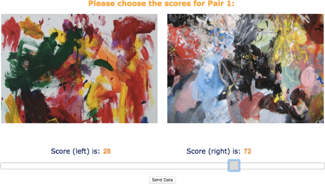
Fig. 1 Group allocation: painting pair 1. Notes: Subjects can move the grey slider. The sum of appreciation units is 100. The default position is at 50–50

After subjects have been reallocated across the two laboratories, they read the instructions for the second part of the experiment. The purpose of the second part is to create stronger social ties between subjects in the same laboratory than those between two subjects in distinct laboratories. The procedures used follow those introduced in Robalo et al. (Reference Robalo, Schram and Sonnemans2017). There are three tasks: first, subjects choose a slogan for their own laboratory to be selected from three options. They do so by chatting without time constraint via a chat box that is only available to subjects in the same laboratory.Footnote ⁹ The group decision is made via majority rule. Subjects are informed that the chosen slogan will be shown on their computer monitors for the remainder of the experiment.

The second task in this part 2 is a tournament between the two laboratories. This aims at further strengthening the social ties within the laboratory. Each subject individually reviews five pairs of paintings and is asked to determine the sources of the paintings in each pair; see Fig. 2 for an example. They are told that each painting may have been made by a child under the age of 15 or by a professional artist.Footnote ¹⁰ There are four possible answers for each pair (both by children; left by child, right by professional, etc.). For each correct answer by an individual, the accumulated score of the laboratory as a whole increases by one. The laboratory with the higher final score receives 24 points as a prize to be divided equally amongst the twelve subjects in that laboratory.

The final task in part 2 is an other-other dictator allocation task. Each subject is asked to allocate two points (in increments of 0.1) between a random participant in the own laboratory (excluding herself) and a random participant in the other laboratory. This provides an alternative measure for the closeness a subject feels towards someone in the own laboratory compared to someone in the other laboratory other than a direct question regarding closeness (see question 5 in exit survey in Appendix A in Electronic supplementary material file). It is an indication of the social ties with co-members relative to the others.

Fig. 2 Group tournament. Notes: Screenshot of the first pair of paintings in the group tournament. The painting on the left is by the 11-year-old Yavagina M. from Minsk, Belarus. The painting on the right is by Sam Gilliam “coffee thyme”. The correct answer is then that the left is painted by a child and the right by a professional painter

To avoid possible spillovers to part 3 of the experiment, the results for the tournament and other-other allocation are revealed only at the end of the experiment. All decisions are paid, including the group tournament, other-other allocation, and the payoffs in the bribery game that is introduced in the next section.

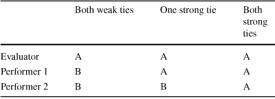
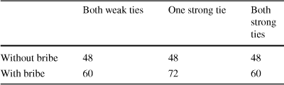
To inform them about the composition of the triads, subjects are told from which laboratory are the evaluator and the other performer. There are three possible compositions. Denote the evaluator’s laboratory by ‘A’; then any performer from laboratory A is defined to have a strong social tie to the evaluator. Any performer from the other laboratory (B) has a weak social tie to the evaluator. This yields the three triad compositions summarized in Table 1, where we label the name of the treatment groups according to the performers’ relationships to the evaluator. Note that having 12 subjects in each of the two laboratories allows us to form exactly 8 triads in each of the treatments. Combining the social-tie treatment with the bribe/no-bribe treatment dimension, Table 2 illustrates all treatment cells and lists the number of subjects in each.

Table 1 Triad composition

	Both weak ties	One strong tie	Both strong ties
Evaluator	A	A	A
Performer 1	B	A	A
Performer 2	B	B	A

A and B refer to laboratory A and laboratory B. We define laboratory A as the evaluator’s laboratory. (1) Both weak ties: the evaluator comes from one laboratory, both performers from the other; (2) One strong tie: the evaluator and one of the performers are from one laboratory, the other performer is from the other laboratory; (3) Both strong ties: all three players are from the same laboratory

Table 2 Number of subjects in treatment groups

	Both weak ties	One strong tie	Both strong ties
Without bribe	48	48	48
With bribe	60	72	60

3.2 The bribery game

The third part of the experiment is a bribery game with a general structure similar to Gneezy et al. (Reference Gneezy, Saccardo and van Veldhuizen2018). Each performer receives a 5-points endowment. Then, all performers conduct the real-effort task developed by Weber and Schram (Reference Weber and Schram2016); their results are sent to the evaluator in their triad. Subsequently, the evaluator selects one winner from the two performers. The winner receives an additional 10-points reward. The evaluator receives a fixed payoff of 10 points.

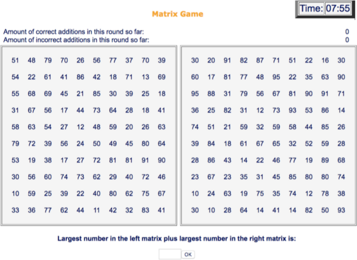
Fig. 3 Matrix task. Notes: A screenshot of the matrix task. Performers are given 8 min to solve as many matrices as possible. Subjects need to find the highest number in each matrix and calculate the sum. The program allows them to see the number of correct and incorrect answers. In this example, the correct answer should be 186 (= 91 + 95). Numbers are generated randomly in a way that puts lower probability on high numbers (to avoid a high probability that the maximum number is above 90); more information is available upon request

3.2.1 Task

Performers in this part are asked to find the sum of the largest numbers in two $10 \times 10$ matrices (Fig. 3). Each cell in these matrices contains a two-digit number between 01 and 99. The task is to find the highest numbers in each of the two matrices and add them up. After entering a number, a new pair of matrices appear, independently of whether the previous answer is correct.Footnote ¹¹ The two performers are given 8 min to solve as many of these matrix puzzles as possible (with a maximum of 30). A running digital clock reminds performers of the time. When time is up, a page pops up showing their own number of correct answers, but not the number of correct answers for the other performer. There is no payoff directly associated with correct answers.Footnote ¹²

After performers have finished the matrix puzzle and seen their own performance in the task, we reveal the social ties between the members of the triad by revealing to which laboratory each belongs. In the bribe treatments, performers are then informed that they may transfer points to the evaluator. Subsequently, each performer sends her result (and transfer points, in the bribe treatments) to the evaluator.Footnote ¹³ The evaluator sees the results and transfers from both performers and selects a winner. Each performer remains unaware of the performance and transfers of the other performer.

Performers may transfer any amount between zero and ten points.Footnote ¹⁴ The evaluator is aware of the social ties with both performers when selecting a winner. It is common knowledge that the transfers are non-refundable, there is no punishment to transferring points (which we interpret as a bribe), and that it is up to the evaluator to select a winner. In summary, the evaluator selects a winner knowing the number of correct answers by the two performers, the transfers from both performers, and her social ties with both performers.

Performers’ transfer decisions are made only once. To collect more observations from evaluators we ask them to make two rounds of decisions. After selecting a winner from the first pair of performers, we ask the evaluators to again select a winner from a different pair of performers. These are randomly chosen and with the same triad composition (in terms of social ties) as in the first round. Evaluators are informed about the second round of decisions only after they have made the decisions for the first round. All participants are informed that the final payment is determined by the decisions in one randomly chosen round.

Before we reveal any results from the experiment, we elicit (incentivized) beliefs of the performers about other performers’ ability to solve the matrix game. Performers guess the distribution of the correct number of answers in their session, i.e., how many performers manage to solve only one task, how many solve two tasks, etc. The closer their guesses are to the observed distribution in their session, the higher their payoff will be. They have five experimental points as an initial endowment, and we subtract 0.25 points for every unit deviation (in number of correct sums) between their answer and the correct answer (see question 6 in the exit survey in Appendix A in Electronic supplementary material file for more information). Finally, we also collect information on socio-economic characteristics and their subjective attachment or closeness towards in-group and out-group members. For the latter, subjects were asked to indicate on a ten-point scale how close they feel to their own laboratory and to the other laboratory, ranging from “don’t feel any attachment” to “really feel like belonging” (see question 5 of the exit survey in Appendix A in Electronic supplementary material file).

In summary, the earnings are determined as follows. Aside from a seven euros show-up fee, a performer’s earning is composed of five parts: the award from the inter-laboratory tournament if her laboratory wins, earnings from the other-other allocation task, five points of fixed payoff as a performer in the bribery game minus the transfer she offers to the evaluator, the ten-point award of being selected the winner in the bribery game (zero if she loses), and earnings from the post-experimental belief elicitation. A evaluator’s earning is also composed of four parts on top of the show-up fee; namely, the award in the tournament if her laboratory wins, money from the other-other allocation task, ten points of fixed payoff as an evaluator in the bribery game, and bribes from both performers. In treatments without bribes performers are not given an opportunity to transfer money to the evaluator and evaluators only receive the fixed wage.

3.3 Conjectures

Denote the fraction of possible occasions that the award is given to the better performer by $ϕ$ . Our point of departure is that, by-and-large, when there are no differences in performers’ bribes or social ties with the evaluator, then $ϕ$ is close to 1. We designed this experiment with the idea that bribe-based and tie-based corruption both bias an evaluator’s decision, in favor of, respectively, the higher briber and stronger tie. Let $B_{+}$ ( $B_{-}$ ) denote the bribe by the better (worse) performer. This yields the following conjectures.

Conjecture 1

Bribe-based corruption

When the better performer bribes less than the worse performer, the fraction of prizes awarded to the better performer is lower than when the better performer bribes as least as much as the worse performer. That is, $ϕ_{| [B_{+} < B_{-}]} < ϕ_{| [B_{+} \geq B_{-}]}$ .

Conjecture 2

Tie-based corruption

In the treatment with one strong tie and without bribes, better performers are less likely to be awarded the prize when they have a weak tie than when they have a strong tie. That is, $ϕ_{[w e a k t i e]} < ϕ_{[s t r o n g t i e]}$ .

We do not have a firm expectation with respect to the relationship between bribe-based and tie-based corruption. They may be complements or substitutes. In fact, this interaction is at the core of our research question.

4 Results

In this section, we first validate our creation of social ties and then present a general overview of our results. Subsequently, we test for treatment effects; we check whether performers’ bribes and evaluators’ corruption vary with the constellation of social ties in the performers-evaluator triads. Unless indicated otherwise, test results are based on permutation t-tests (indicated by 1 − PtT for one-sample tests and 2 − PtT for two-sample tests). These are non-parametric tests for differences in means (note that the often used Wilcoxon and Mann–Whitney tests test more generally for differences in distributions). As argued by Moir (Reference Moir1998) and Schram et al. (Reference Schram, Brandts and Gerxhani2019), such permutation tests have higher power than many alternatives.

4.1 Creating social ties

Our manipulation of social ties successfully created ties of different strength. Figure 4 presents two measures. We use measures for the subjective closeness collected in the post-experimental questionnaire (measured on a 10-point scale) as the main proxy for social ties. It is shown in the left panel in Fig. 4 that the median feeling of closeness towards someone with whom one has strong ties is five out of ten, while it is two out of ten towards someone with whom one shares only weak ties. The difference between the two groups is statistically highly significant (1 − PtT, $p < 0.001$ , $N = 336$ ). Our alternative measure of social ties confirms that subjects treat those from their own group better than those from the other group. Recall that each subject is asked to divide two points (in 0.1 point increments) between a random in-group member and a random out-group member in the other-other allocation task. The observed allocations are shown in the right panel. The points that subjects allocate are presented on a scale of 0 to 20. The results show that the median amount of money allocated to a random member in the same laboratory is three times more than that distributed to a random member in the other laboratory. The amount allocated to someone with whom one has strong ties is significantly higher than 10 (which would imply an equal split), (1 − PtT, $p < 0.001$ , $N = 144$ ).Footnote ¹⁵

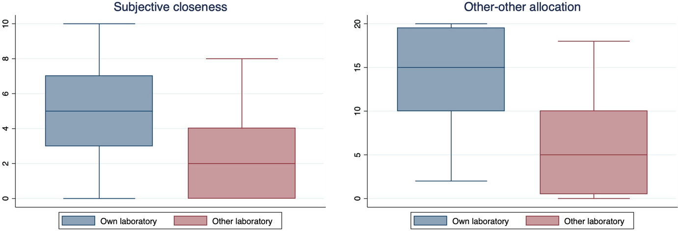
Fig. 4 Social tie manipulation. Notes: The left panel illustrates the subjective feelings of closeness towards members in the same and other laboratory as expressed in the post-experimental questionnaire. The right panel shows the results of the ‘other-other allocation’ task. Subjects are asked to distribute 2 points in 0.1 point increments between a random other participant in the same laboratory and a random participant in the other laboratory. The results are shown on a scale from 0 to 20. Upper and lower bounds indicate the maximum and minimum observed values; boxes depict 25–75 percentiles and the horizontal line gives the median observation

4.2 General overview

Randomization: We have data on 224 performers, of which 128 are in the Bribery treatment and 96 in the No-Bribery treatment. There are 108 evaluators, 60 in the Bribery treatment and 48 in the No-Bribery treatment.Footnote ¹⁶ Table D1 in Appendix D in Electronic supplementary material file presents descriptives for the participants in the various treatments. Pairwise differences across treatments in age, gender, and a variable measuring a major in economics or business are all insignificant at the 5% level (2 − PtT). Additional evidence of successful randomization comes from comparing performance (that is, the number of correct summations) in the two laboratories. Mean performance in the two laboraties was 7.58 and 7.48. The difference is statistically insignificant (2 − PtT, p = 0.852). Table 3 shows performance across treatments. The average number of correct matrix summations is between 7 and 8 and does not seem to vary much across treatments. Indeed, we find no statistically significant difference in task performance (all pairwise comparisons, $p > 0.1$ , 2 − PtT).Footnote ¹⁷ Recall that while doing the task, subjects are unaware of any of the features that distinguish between the treatments. This result, then, is an indication of a successful randomization of subjects across treatments.

Table 3 Descriptive statistics

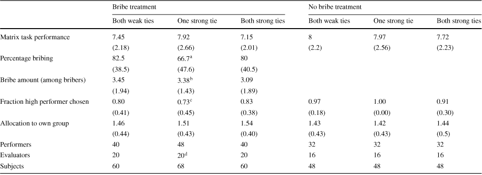
	Bribe treatment			No bribe treatment
	Both weak ties	One strong tie	Both strong ties	Both weak ties	One strong tie	Both strong ties
Matrix task performance	7.45	7.92	7.15	8	7.97	7.72
Matrix task performance	(2.18)	(2.66)	(2.01)	(2.2)	(2.56)	(2.23)
Percentage bribing	82.5	66.7 $^{a}$	80
Percentage bribing	(38.5)	(47.6)	(40.5)
Bribe amount (among bribers)	3.45	3.38 $^{b}$	3.09
Bribe amount (among bribers)	(1.94)	(1.43)	(1.89)
Fraction high performer chosen	0.80	0.73 $^{c}$	0.83	0.97	1.00	0.91
Fraction high performer chosen	(0.41)	(0.45)	(0.38)	(0.18)	(0.00)	(0.30)
Allocation to own group	1.46	1.51	1.54	1.43	1.42	1.44
Allocation to own group	(0.44)	(0.43)	(0.40)	(0.43)	(0.43)	(0.5)
Performers	40	48	40	32	32	32
Evaluators	20	20 $^{d}$	20	16	16	16
Subjects	60	68	60	48	48	48

Task performance refers to the number of matrix pairs correctly solved. Treatments are defined in Sect. 3.1. ‘Allocation to own group’ is the amount allocated to a random other of the own group when dividing two points with a random participant in the other group

$^{a}$ For player with the strong tie: 70.8 (46.4); for player with the weak tie: 62.5 (49.4). This difference is statistically insignificant (2 − PtT, $p = 0.763$ )

$^{b}$ For player with the strong tie: 3.41 (1.54); for player with the weak tie: 3.33 (1.34). This difference is statistically insignificant (2 − PtT, $p = 0.904$ )

$^{c}$ If the player with the strong tie performs as least as well as the other: 0.82 (0.39); if the player with the weak tie performs better than the other: 0.61 (0.51). This difference is statistically insignificant (2 − PtT, $p = 0.274$ )

$^{d}$ Data for four evaluators were lost due to technical problems in the first session

Bribes: Table 3 also shows bribes across treatments. It reveals that when given the opportunity, most subjects send a bribe. The average amount bribed (conditional on sending a bribe) varies little across treatments. More specifically, more than 66% of the performers send money to evaluators even though bribes are non-refundable. In ‘Both weak ties’ and ‘Both strong ties’, the bribe rate goes up to 82.5% and 80.0%, respectively, but neither is statistically different at the 5% level from the 66% observed in the ‘One strong tie’ treatment (‘Both weak tie’ vs. ‘One strong tie’: $p = 0.09$ , ‘Both strong tie’ vs. ‘One strong tie’: $p = 0.16$ , 2 − PtT).Footnote ¹⁸ On average bribers— conditional on the decision to bribe—give more than three points to the evaluator (Table 3). We observe no statistically significant differences across treatments in the conditional amount bribed.Footnote ¹⁹ Finally, as indicated in the table note, bribes do not differ much between the two performers in the treatment with one strong and one weak tie. Of course, the lack of an effect of social ties on bribing behavior might be due to the method used to induce ties. Perhaps social ties in the world outside the laboratory are stronger and do induce differential bribing behavior. On the other hand, we will see that the ties we induce do affect corruption. This suggests that such ties can have real consequences for participants’ decisions, even if they do not affect bribing choices.

Corruption: There are two situations in which we consider an evaluator’s decision to be corrupt. First, a decision is ‘bribe-based corrupt’ if it awards the prize to the worse performer when her bribe is higher.Footnote ²⁰ The second type is ‘tie-based corruption’. This may occur (only) in the treatment where one of the performers has a strong tie with the evaluator and the other has a weak tie, while the better performer bribes the same amount or more than the other. If the better performer has the weak tie and the other receives the prize, we consider this tie-based corruption; in spite of the fact that the performer with the weak tie performs better and bribes as least as much, the prize is allocated to the performer with a strong tie.Footnote ²¹ We have a total of 82 performer pairs where neither bribes nor performance were tied. In 42 of these cases (51%), the performer that performed poorer bribed more, thus creating scope for bribe-based corruption.Footnote ²² In the treatment with one strong tie, there were 26 cases where the better performer bribed as least as much as the other. This creates the possibility of tie-based corruption.

Figure 5 plots, by treatment, the mean fraction of times in which the evaluator awarded the prize to the better performer. For this analysis, we disregard performer pairs with equal performance (contrary to the corresponding row in Table 3). The figure distinguishes between cases where the better performer bribed less than, equal to, or more than the lower performer. The black bars (lower bribes by the better performer) represent the 38 cases where bribe-based corruption is possible. Indeed, corruption is observed in these cases; the better performer is not always the one to whom the prize is awarded. In aggregate, bribe-base corruption is observed in 53% of the cases where it is possible. Aside from the black bars, the only two cases where the poorer performer is sometimes awarded the prize are in the treatment with one strong and one weak tie, while the better performer bribes at least as much as the other. Of these 26 cases, there are 12 where the better performer has the weak tie, which opens the possibility of tie-based corruption. Such corruption is observed in four of these cases (33%).Footnote ²³ These first results suggest that bribe-based corruption is a more important phenomenon than tie-based corruption; below, we will study in more detail how evaluators weigh bribes and social ties. Finally, note that in all (34) cases where neither type of corruption is possible, the prize was awarded to the better performer. Together, these results provide support for Conjectures Footnote ¹ and Footnote ². The regressions to be presented below show that these results are statistically significant.

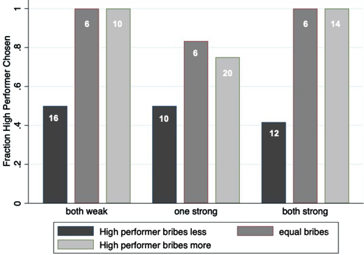
Fig. 5 Fraction of Better Performers Chosen. Notes: Bars show fraction of times that the high performer is awarded the prize. Numbers in the bars denote the numbers of observations. The horizontal axis depicts for each treatment whether the high performer bribed less than, equal to, or more than the low performer. Bribe-based corruption can occur only when the high performer bribes less (black bars). Tie-based corruption can occur only when there is one strong and one weak tie. In both cases, corruption is stronger, the lower is the bar

4.3 Treatment effects

Now we turn to the main research question; how do social ties interact with bribery and corruption? We first consider the treatment effects on performers’ decision, that is, the decision to bribe and the amount bribed and subsequently discuss the effects on evaluators’ corruption.

4.3.1 Bribes

Recall that we found no apparent treatment effects on bribes in Table 3, that is, neither at the intensive nor at the extensive margin do our social tie treatments seem to affect bribing behavior. The aggregation level used there, however, might gloss over more subtle differences. For example, we have not yet considered the distinct bribing behavior between the two performers when one has a strong tie to the evaluator and the other a weak tie.

We first consider in Table 4 the Pearson correlations between bribing, performance, beliefs about the other’s performance, and the treatment dummy variables. For the treatment with one weak and one strong tie we consider the two performers separately. Most of the correlations considered are weak and statistically insignificant.

Table 4 Correlations

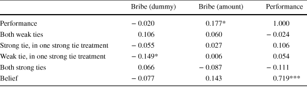
	Bribe (dummy)	Bribe (amount)	Performance
Performance	− 0.020	0.177*	1.000
Both weak ties	0.106	0.060	− 0.024
Strong tie, in one strong tie treatment	− 0.055	0.027	0.106
Weak tie, in one strong tie treatment	− 0.149*	0.006	0.054
Both strong ties	0.066	− 0.087	− 0.111
Belief	− 0.077	0.143	0.719***

‘Bribe (dummy)’ is 1 if the performer bribed. ‘Bribe (amount)’ is the amount bribed conditional on bribing. ‘Performance’: number of correct matrix sums. ‘Strong social tie’: the performer in the one-social-tie treatment with a strong social tie to the evaluator. ‘Belief’: expected number of correct summations by the other performer. Cells give the Pearson correlation coefficient; t-tests test the difference with correlation 0. * $p < 0.1$ , ** $p < 0.05$ *** $p < 0.01$

The second and third columns show that the decision to bribe (extensive margin) and the amount bribed (intensive margin) are both uncorrelated with the two treatments where the performers share the same tie. More specifically, all four correlation coefficients between the propensity to bribe or the amount bribed on the one hand and the ‘both weak ties’ and ‘both strong ties’ dummies on the other hand are statistically insignificant and below 0.11. Performers with the weak tie when the other has a strong tie to the evaluator bribe (marginally) significantly less often.Footnote ²⁴ The amount bribed is marginally significantly correlated with one’s performance in the matrix task. The positive correlation indicates that participants who perform well tend to transfer higher amounts if they bribe. The fourth column confirms our earlier observation that performance does not correlate with the treatments. Finally, the last row shows the correlations between elicited beliefs about the other performer’s score and the own bribe and performance. It shows that a better own performance correlates with a higher expected performance by the other. This belief, however, is not significantly correlated with the likelihood or level of bribing.

To complete the analysis of bribes, we regress the extensive and intensive margins of bribery on a set of treatment dummies and individual characteristics. Table 5 presents the results of a hurdle model combining a probit regression of performers’ decision on whether to bribe or not with a linear regression of the amount bribed conditional on bribing. The independent variables for the probit equation include treatment dummies, being the strong-tie performer in the ‘One strong tie’ treatment, performance, beliefs and interaction terms. For the linear equation, we add a set of individual characteristics.

We use the weak-tie performer in the ‘One strong tie’ treatment as the baseline. Compared to this performer we observe that (i) someone who also has a weak tie but is paired with another weak-tie performer (that is, someone in the ‘Both weak tie’ treatment) is more likely to bribe; and (ii) the effect of performance on the likelihood of bribing is stronger for her strong-tie partner. Both of these effects are marginally significant. The strongest effect of ties on bribes is observed for the role of beliefs. Beliefs about the partner’s performance do not significantly affect bribes for the baseline group, nor for the treatments where both performers share the same tie to the evaluator. In the ‘One strong tie’ treatment, we observe somewhat surprisingly that the performer with a strong tie is less likely to bribe, the higher is the performance she expects from the other. The big picture, however, is that there is very little evidence that bribes offered by the performers are affected by the social ties between the performers and the evaluator.

Table 5 Performers’ bribe behavior: hurdle model regression

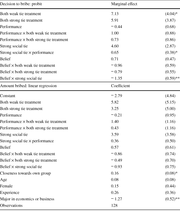
Decision to bribe: probit	Marginal effect
Both weak tie treatment	7.13	(4.04)*
Both strong tie treatment	5.91	(3.87)
Performance	$-$ 0.44	(0.68)
Performance $\times$ both weak tie treatment	1.00	(0.88)
Performance $\times$ both strong tie treatment	0.73	(0.86)
Strong social tie	4.60	(2.87)
Strong social tie $\times$ performance	0.65	(0.38)*
Belief	0.71	(0.47)
Belief $\times$ both weak tie treatment	$-$ 0.96	(0.59)
Belief $\times$ both strong tie treatment	$-$ 0.79	(0.55)
Belief $\times$ strong social tie	$-$ 1.35	(0.59)**

Amount bribed: linear regression	Coefficient
Constant	$-$ 2.79	(4.84)
Both weak tie treatment	5.82	(5.15)
Both strong tie treatment	3.25	(5.00)
Performance	$-$ 0.21	(0.95)
Performance $\times$ both weak tie treatment	1.40	(1.16)
Performance $\times$ both strong tie treatment	0.43	(1.16)
Strong social tie	3.59	(3.58)
Strong social tie $\times$ performance	0.36	(0.50)
Belief	0.57	(0.61)
Belief $\times$ both weak tie treatment	$-$ 0.86	(0.74)
Belief $\times$ both strong tie treatment	$-$ 0.49	(0.70)
Belief $\times$ strong social tie	$-$ 0.93	(0.75)
Closeness towards own group	0.16	(0.08)*
Age	0.08	(0.08)
Female	0.15	(0.44)
Experience	0.26	(0.36)
Major in economics or business	$-$ 1.27	(0.52)**
Observations	128

‘Performance’: number of correct matrix sums. ‘Strong social tie’: the performer in the one-social-tie treatment with a strong social tie to the evaluator. ‘Belief’: expected number of correct summations by the other performer. ‘Experience’: number of previous experiments the performer had participated in. * $p < 0.1$ , ** $p < 0.05$ *** $p < 0.01$

4.3.2 Corruption

We therefore now turn to investigating treatment effects in evaluators’ corruption. To capture how evaluators choose a winner from two candidate performers under varying constellations of social ties, we apply McFadden’s conditional logit analysis (McFadden Reference McFadden and Zarembka1973). This allows us to investigate how evaluators value performers based on different attributes of the performers themselves, including performance, bribes, and social ties to the evaluator. Since each evaluator in our experiment is asked to rate winners in two rounds, we have two observed choices for each evaluator. We will therefore cluster standard errors at the level of the evaluator.

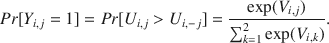
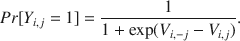
More specifically, suppose that evaluators have a random utility framework (Manski Reference Manski1977) as defined in equation (1):

(1)

\begin{matrix} U_{i, j} = V_{i, j} + ε_{i, j}, \end{matrix}

where evaluator i attributes (random) utility $U_{i, j}$ , $i = 1, \dots, N$ to performer $j \in 1, 2$ . Utility is composed of a deterministic term $V_{i, j}$ , that depends on observed performer characteristics; and a random term $ε_{i, j}$ . Let $Y_{i, j} = 1$ denote that evaluator i prefers performer j over the other performer $- j$ in her triad. Assuming that $ε$ follows a type-I extreme value distribution (Luce Reference Luce2005) this yields the probability that performer j is preferred by evaluator i

(2)

\begin{matrix} P r [Y_{i, j} = 1] = P r [U_{i, j} > U_{i, - j}] = \frac{exp (V_{i, j})}{\sum_{k = 1}^{2} exp (V_{i, k})} . \end{matrix}

To proceed, we assume a linear function for the latent variable $V_{j}$ (for ease of notation we drop the subscript i for the evaluator). Then the value of performer j is assumed to be given by a linear combination of observable characteristics:

(3)

\begin{matrix} V_{j} & = α + β_{1} P e r f o r m_{j} + β_{2} T i e_{j} + β_{3} P e r f o r m_{j} \times T i e_{j} \\ + β_{4} B r i b e_{j} + β_{5} B r i b e_{j} \times T i e_{j} + β_{6} Z_{j}^{'} + ε_{j}, \end{matrix}

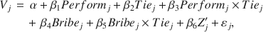
where $P e r f o r m_{j}$ is the number of correct summations, $B r i b e_{j}$ is the amount bribed (only used in the bribe treatments), $T i e_{j}$ is a dummy variable indicating that the performer has a strong tie to the evaluator, $\times$ indicates an interaction effect, and $Z_{j}^{'}$ denotes a vector of personal characteristics. Substituting equation (3) into equation (2), the probability that performer j is preferred to performer $- j$ by the evaluator is given by

(4)

\begin{matrix} P r [Y_{i, j} = 1] = \frac{1}{1 + exp (V_{i, - j} - V_{i, j})} . \end{matrix}

Equation (4) is the model we seek to fit.Footnote ²⁵ Since performers in the ‘Both strong ties’ and ‘Both weak ties’ treatments have the same social ties to the evaluator there is no difference between the two performers in this respect (the terms drop out of $V_{i, - j}$ – $V_{i, j}$ ). Moreover, personal characteristics of an evaluator are stable across her valuation of the performers so they do not enter the estimation equation. We estimate the combination of model (4) and (3) separately for treatments with and without bribes. Table 6 reports the estimated coefficients.

Table 6 The effect of performance and bribes on the chance of winning

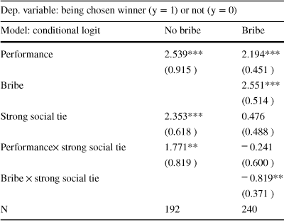
Dep. variable: being chosen winner ( $y = 1$ ) or not ( $y = 0$ )
Model: conditional logit	No bribe	Bribe
Performance	2.539***	2.194***
Performance	(0.915 )	(0.451 )
Bribe		2.551***
Bribe		(0.514 )
Strong social tie	2.353***	0.476
Strong social tie	(0.618 )	(0.488 )
Performance $\times$ strong social tie	1.771**	$-$ 0.241
Performance $\times$ strong social tie	(0.819 )	(0.600 )
Bribe $\times$ strong social tie		$-$ 0.819**
Bribe $\times$ strong social tie		(0.371 )
N	192	240

The unit of observation is the single performer. The dependent variable is whether or not the evaluator selects the performer to be the winner. Performance and bribe are both standardized. ‘Strong social tie” is a dummy variable which equals 1 if the performer has a strong social tie to the evaluator. Recall that this only enters the regression if the other performer has a weak tie to the evaluator. Conditional logit regression coefficients are reported. Robust standard errors between parentheses allow for clustering at the level of an evaluator. * $p < 0.1$ , ** $p < 0.05$ , *** $p < 0.01$

The coefficients in Table 6 reflect the direction and weights that the evaluator puts on the attributes when valuing two performers (Long and Freese Reference Long and Freese2006); a positive coefficient indicates that the evaluator values a higher score on the attribute concerned. The larger the coefficient is, the higher is the weight that the evaluator puts on the attribute. $β_{1}$ represents the effect on the evaluator’s decision of the performance of a performer in a treatment where two performers have the same social ties with the evaluator (see eq. 3). Similarly, $β_{4}$ measures the importance of bribes by that performer. The marginal effect of performance when being the only performer with a strong social tie to the evaluator is measured by $β_{1} + β_{3}$ ; the effect of her bribes is reflected by $β_{4} + β_{5}$ .

The results for the treatment without bribes show that both performance and social ties to the evaluator contribute positively to the chance of being selected as the winner.Footnote ²⁶ The effects are of a similar magnitude. Not only do both performance and social ties have an effect, they also reinforce each other. Performance of those with a (sole) social tie to the evaluator is rewarded at a significantly higher rate than for those without such a tie.

Now consider the situation where bribes are possible. Here, performance is somewhat less important than when bribes are not allowed. Moreover, for the effects of performance, being the only performer with a strong social tie is a further disadvantage. For these performers there is, however, still a significant effect of performance on the chances of winning the prize.Footnote ²⁷ Bribes increase the probability of being awarded the prize (which confirms Conjecture Footnote ²). Though this effect is significantly weaker for those with a (sole) strong social tie to the evaluator, bribes have a significantly positive effect for these performers as well.Footnote ²⁸. Note that the negative effect of the interaction term between Bribe and Strong Social Tie provides an answer to our main research question; bribes and social ties are substitutes.

To test the differences in the effects of strong social ties with and without the possibility of bribes, we conducted the conditional logit analysis for all treatments combined.Footnote ²⁹ We first set bribes in the non-bribe treatment to zero and created a dummy variable indicating the bribe treatment. To the regression equation for the treatment with bribes, we then added the interaction between the new dummy and the strong social tie dummy (note that we cannot add the bribe dummy itself because there is no within-pair variation). We also added the triple interaction between the bribe treatment dummy, strong social tie, and performance. The results for the variables reported in Table 6 remain qualitatively the same. For the interaction between the bribe-treatment dummy and having a strong social tie, the coefficient is $- 1 . 78^{* *}$ . The triple interaction term has coefficient $- 2 . 15^{* *}$ . This shows that the differences between the columns of Table 6 in the corresponding coefficients are statistically significant. More details are available upon request.

Table 7 illustrates the size of the effects implied by the coefficients reported in Table 6. Numbers show the estimated probability of winning for a performer in various circumstances. In all cells, the ‘other’ performer is assumed to have a weak social tie to the evaluator and mean performance and bribe. When bribes are not possible, simply having a strong social tie to the evaluator increases one’s likelihood of winning by 41%-points to 91%. The social-tie effect is much smaller at 62% when bribes are possible. Increased performance also leads to a very high chance of winning when there are no bribes. When a performer has a strong social tie to the evaluator (and the other performer does not), having a one-standard-deviation better performance makes winning the prize virtually certain. Even with a weak social tie, a better performance leads to a very high chance of winning (93%).Footnote ³⁰ These effects of performance are slightly weaker when bribes are possible, but—without difference in bribe—outperforming the other still leads to a very high chance of winning. Other things equal, a one-standard-deviation higher bribe than the other performer has an effect that is similar in magnitude to the one-standard-deviation effect of a better performance. All in all, the possibility of bribes crowds out the role of social ties and allows performers to compensate poor performance by bribing more than the other.

Table 7 Estimated probability of winning

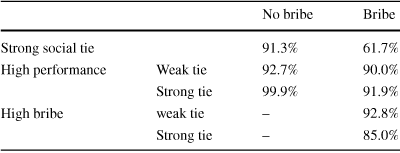
		No bribe	Bribe
Strong social tie		91.3%	61.7%
High performance	Weak tie	92.7%	90.0%
High performance	Strong tie	99.9%	91.9%
High bribe	weak tie	–	92.8%
High bribe	Strong tie	–	85.0%

If both performers have equal performance, social tie to the evaluator, and bribe, then each has a probability of 50% of being awarded the prize. The cells show a performer’s probability of winning if she has a strong social tie to the evaluator, or has a performance or bribe that is one standard deviation above the mean. The other performer is assumed to remain without strong social tie to the evaluator and have mean performance and bribe

5 Concluding remarks

We use a laboratory experiment to examine the interaction between social ties and corruption. After generating social ties, triads of players enter a real-effort bribery game where one evaluator selects one of two performers as the winner of a prize. There are three possible constellations of social ties between the evaluator and the performers. This allows us to draw conclusions about the causal relationship between on the one hand such ties and on the other hand performers’ decisions to bribe and evaluators’ corrupt behavior. We find that social ties have a strong effect on evaluators’ decisions. When bribing is not an option, evaluators’ decisions exhibit a strong tendency to give preferential treatment to those with whom they share a strong social tie. When the evaluator can be bribed, the effect of strong ties disappear. Now, performance and bribes are both rewarded to a similar extent, while ties have almost no effect on the evaluators’ decisions.

Our experiment is a first step towards a better understanding of how bribe-based corruption interacts with social-tie based corruption. Various extensions to our setup could provide further insights. First, one could extend the environment to allow for a repeated interaction between performers and the evaluator. In the world outside the laboratory, interactions are often not of a one-shot nature. Repetition would introduce reputation concerns (e.g., a reputation of being open to bribes). Secondly, to deter corruption, policies typically include a penalty or other type of punishment. Future research can determine the effect of punishment on bribes. Thirdly, by design, we create a very corrupt environment because the evaluators are ‘forced’ to take both bribes. We made this design choice in order to create an environment in which bribes somehow have become a ‘way of life’ and socially acceptable. Future work could extend on this and allow for rejection of bribes. Though such extensions certainly provide interesting venues for future research, we believe that the experiments discussed here provide valuable insights into the interaction between social distance and corruption. Specifically, the result that bribes crowd out tie-based corruption is important for understanding corruption in the world outside the laboratory. When bribes are possible, ‘old-boys networks’ may be a less important source of corruption than is typically assumed. It should be stressed, however, that the social ties we consider are formed within the minimal-group paradigm. Stronger ties may exist between members of groups that are formed naturally outside of the laboratory (see the examples mentioned in the introduction). Whether stronger ties can also be crowded out by bribes is an open question (note that bribes outside the laboratory are typically also orders of magnitude higher than in our experiments). What our results do show, is that such crowding out is a real possibility.

Though these should be taken with a caveat, some preliminary policy conclusions follow from our results. First, consider environments where strong social ties exist between government officials and business owners or managers, and bribes are common. Our results suggest that policies here might do well in focusing first on stopping the bribes. Second, when bribes are uncommon but social ties are strong, these ties should not be ignored. They may cause a strong bias in government officials’ choices. Finally, a policy that has been becoming more popular in recent years is staff rotation. This aims at reducing the effects of social ties on important public-sector decisions. Though we recognize the role of staff rotation in reducing repeated-game strategies in corruption, our results suggest that such a policy may not reduce corruption if bribes are readily used. In those circumstances, ties are less important for corrupt behavior than bribes.

We believe our results to be generally applicable. An argument can be made, however, that they are especially important for developing countries. As argued in the introduction, bribes are particularly prevalent in the developing world, and social ties dictate business to government relations. We conclude that in these countries, staff rotation, or alternative methods aimed at reducing the effects of social ties are likely to fail in reducing corruption. A first step that is needed is a reduction in the bribes themselves.

Acknowledgements

We owe our gratitude to financial support from the Research Priority Area Behavioral Economics of the University of Amsterdam. Gönül Doğan would like to thank for financial support by the Dr. Jürgen Meyer Stiftung. We also thank Soo Hong Chew, Uri Gneezy, Simin He, Rudy Ligtvoet, Joep Sonnemans, Jeroen van de Ven, Boris van Leeuwen, Matthias Weber, and participants at a CREED internal seminar, the 2014 Morality Incentives and Unethical Behavior Conference in San Diego, the 2015 IMEBESS conference in Toulouse, the ESA North America 2016 meetings, the 2016 BEAT conference at Tsinghua University, the 2017 LISER inaugural workshop, and the 4th Microeconomics conference at Nanjing Audit University in 2017 for valuable comments. Jin Di wants to thank Max Hoyer and Aaron Kamm for help in programming.

Footnotes

Electronic supplementary material The online version of this article (https://doi.org/10.1007/s10683-020-09683-7) contains supplementary material, which is available to authorized users.

¹ A special cast of tie-based corruption is ’nepotism’, where family ties are concerned.

² For a discussion of the use of experiments in the social sciences, see Falk and Heckman (Reference Falk and Heckman2009). Gächter and Schulz (Reference Gächter and Schulz2016) provide interesting evidence of the correlation between laboratory measures of dishonesty and evidence of corruption, tax evasion and fraudulent politics in the field.

³ For an overview from the social-psychology perspective, see Köbis et al. (Reference Köbis, van Prooijen, Righetti and Van Lange2015, Reference Köbis, Iragorri-Carter and Starke2018).

⁴ In studies like Chen and Li (Reference Chen and Li2009), a shared “group identity” is induced simply by grouping subjects based on trivial shared preferences. This is enough to create in-group bias. Here we interpret such “minimal groups” as yielding “minimal social ties”.

⁵ There is also a large literature that studies the related phenomenon of ingratiation, that is, making effort to establish oneself as ‘likeable’ towards someone else. See Robin et al. (Reference Robin, Rusinowska and Villeval2014) for an example and review of this literature.

⁶ The most recent literature review of experiments on corruption appears to be Bobkova and Egbert (Reference Bobkova and Egbert2012), which discusses the original papers like Abbink et al. (Reference Abbink, Irlenbusch and Renner2002), Abbink (Reference Abbink2004), Abbink and Hennig-Schmidt (Reference Abbink and Hennig-Schmidt2006), Barr and Serra (Reference Barr and Serra2009), Cameron et al. (Reference Cameron, Chaudhuri, Erkal and Gangadharan2009). Subsequent laboratory studies include Fahr and Djawadi (Reference Fahr and Djawadi2012); Armantier and Boly (Reference Armantier and Boly2013), Berninghaus et al. (Reference Berninghaus, Haller, Krüger, Neumann, Schosser and Vogt2013), Vetter (Reference Vetter2013), Abbink et al. (Reference Abbink, Dasgupta, Gangadharan and Jain2014), Drugov et al. (Reference Drugov, Hamman and Serra2014), Zhang (Reference Zhang2015), Zhang (Reference Zhang2015), Banerjee (Reference Banerjee2016), Campos-Vazquez and Mejia (Reference Campos-Vazquez and Mejia2016), Fišar et al. (Reference Fišar, Kubák, Špalek and Tremewan2016), Salmon and Serra (Reference Salmon and Serra2017), Abbink et al. (Reference Abbink, Freidin, Gangadharan and Moro2018), Vranka and Bahník (Reference Vranka and Bahník2018), Czap and Czap (Reference Czap and Czap2019), Gneezy et al. (Reference Gneezy, Saccardo and van Veldhuizen2018), Bühren (Reference Bühren2020) and Parra (Reference Parra2020).

⁷ Experimental instructions and questions asked in the exit survey can be found in Appendix A in Electronic supplementary material file.

⁸ See Appendix B in Electronic supplementary material file for more details.

⁹ Appendix C in Electronic supplementary material file provides an example of these chats.

¹⁰ Paintings by professional painters are obtained from MoMA’s online gallery, which are freely available for research purposes. For the children’s paintings, we are grateful to the “Global Children’s Art Gallery” (naturalchild.org/gallery) for granting us permission to use these. All paintings used are shown in Appendix C in Electronic supplementary material file.

¹¹ Success in this task is mainly related to the ability to focus in searching for the highest numbers. Schram et al. (Reference Schram, Brandts and Gerxhani2019) show that there are no gender differences in ability when the task is done in a non-competitive environment.

¹² After having finished the instructions for this part and before starting the task, all subjects have to correctly answer a set of questions testing their understanding of the task, the duties related to being the evaluator or a performer, the payoff scheme, and the time constraint. Before assigning roles to evaluators and performers, all subjects go through a trial session of the matrix puzzle to familiarize themselves with the task.

¹³ We designed the experiment in such a way that performers can only truthfully report their results.

¹⁴ Together with the show up fee of seven euros, the five point starting capital and one-to-one exchange rate ensure that a performer will have positive earnings from participation even if she transfers ten points and has no other earnings.

¹⁵ The dictator allocation measure and the closeness measure are positively and significantly correlated (Pearson’s correlation coefficient is 0.19, p < 0.01 ). Due to technical problems, the other-other allocation data of the first eight sessions were unfortunately lost. Figure 4 therefore plots observations collected in six sessions (144 observations). For this reason, we use the subjective measure in our regression analyses below. These regression results do not change qualitatively or quantitatively if we use the allocation measure instead.

¹⁶ Data on four evaluators in the Bribery treatment are missing due to a programming error in the first session. Performers’ decisions in this session are not affected.

¹⁷ For treatments with bribes, the p values for the pairwise comparisons are: ‘Both weak tie’ vs. ‘One strong tie’ p = 0.55 , ‘Both weak tie’ versus ‘Both strong tie’ p = 0.25 , and ‘One strong tie’ vs. ‘Both strong tie’ p = 0.13 . Without bribes, the pairwise comparisons show no significant differences, either: ‘Both weak tie’ vs. ‘One strong tie’ p = 0.91 , ‘Both weak tie’ vs. ‘Both strong tie’ p = 0.82 , and ‘One strong tie’ vs. ‘Both strong tie’ p = 0.73 .

¹⁸ The bribe rate in our experiment should not come as a surprise. We can compare our rates with those observed in a number of previous studies. Subjects in Abbink et al. (Reference Abbink, Irlenbusch and Renner2002) bribe at a rate of 51–76%, depending on the treatment. Subjects in Abbink (Reference Abbink2004) bribe at a rate of 34–51% while those in Abbink and Hennig-Schmidt (Reference Abbink and Hennig-Schmidt2006) show rates of 48–51%. The bribe rate is 63–87% in Barr and Serra (Reference Barr and Serra2009). Finally, in a treatment group in Gneezy et al. (Reference Gneezy, Saccardo and van Veldhuizen2018) to check for robustness where the task is objective, a bribe rate of 64% is observed.

¹⁹ ‘Both strong ties’ vs. ‘one strong tie’: p = 0.889 ; ‘one strong tie’ vs ‘both weak ties’: p = 0.543 ; ‘both weak ties’ vs. ‘both strong ties’: p = 0.475 , all 2 − PtT. As reported in the table note, in the treatment with one strong tie we also find no significant differences in bribes between the two performers.

²⁰ Note that the evaluator’s decision cannot be explained by greed, because she keeps bribes from both performers by design. Corruption might, however, be motivated by reciprocity, where rewarding the higher transfer is more important to the evaluator than rewarding performance.

²¹ If in the one-strong-tie treatment the better performer bribes less than the other and has a weak tie, then both types of corruption might cause the evaluator to allocate the prize to the other performer. For sake of simplicity, we categorize this as bribe-based corruption.

²² Because of the data recording problems in the first session (mentioned above), we do not have the evaluator’s decisions for four of these cases.

²³ Somewhat surprisingly, there were also two cases where the performer with a strong tie to the evaluator performed better and bribed at least as much, but the prize was awarded to the performer with a weak tie.

²⁴ This correlation compares those with a weak tie to all other performers. If we only consider participants in the ‘One strong tie’ treatment, the correlation drops to 0.088, with p = 0.55 .

²⁵ Note that the constant term a in (3) drops out of the equation in (4). In other words, the intercept plays no role in the conditional probability of performer j being preferred over - j . For this reason, there is no intercept in our estimation.

²⁶ The significant effect for a strong social tie provides support for Conjecture Footnote ¹.

²⁷ The effect of a marginal increase in performance is given by β 1 + β 3 ; this remains significantly different from zero ( χ 2 ( 1 ) = 2.45 , p = 0.001 ).

²⁸ For this group, the effect of a marginally higher bribe is given by β 4 + β 5 . This is significantly larger than zero ( χ 2 ( 1 ) = 11.91 , p = 0.001 ).

²⁹ We thank editor Marie-Claire Villeval for suggesting this analysis.

³⁰ The result that in the absence of bribes and tie differences performance is rewarded so strongly is a clear indication that evaluators consider it a natural choice to reward the better performer.

Springer Nature remains neutral with regard to jurisdictional claims in published maps and institutional affiliations.

References

Abbink, K (2004). Staff rotation as an anti-corruption policy: An experimental study. European Journal of Political Economy, 20(4), 887–906. 10.1016/j.ejpoleco.2003.10.008CrossRef Google Scholar

Abbink, K, Dasgupta, U, Gangadharan, L, & Jain, T (2014). Letting the briber go free: An experiment on mitigating harassment bribes. Journal of Public Economics, 111, 17–28. 10.1016/j.jpubeco.2013.12.012CrossRef Google Scholar

Abbink, K, Freidin, E, Gangadharan, L, & Moro, R (2018). The effect of social norms on bribe offers. The Journal of Law, Economics, and Organization, 34(3), 457–474. 10.1093/jleo/ewy015CrossRef Google Scholar

Abbink, K, & Hennig-Schmidt, H (2006). Neutral versus loaded instructions in a bribery experiment. Experimental Economics, 9(2), 103–121. 10.1007/s10683-006-5385-zCrossRef Google Scholar

Abbink, K, Irlenbusch, B, & Renner, E (2002). An experimental bribery game. Journal of Law, Economics, and Organization, 18(2), 428–454. 10.1093/jleo/18.2.428CrossRef Google Scholar

Angelucci, M., De Giorgi, G., & Rasul, I. (2016). Consumption and Investment in Resource Pooling Family Networks. Working Paper.Google Scholar

Armantier, O, & Boly, A (2013). Comparing corruption in the laboratory and in the field in burkina faso and in Canada. The Economic Journal, 123(573), 1168–1187. 10.1111/ecoj.12019CrossRef Google Scholar

Arusha, RDC, & Schneider, F (2017). How does corruotion affect public debt? An empirical analysis. World Development, 90, 115–127. 10.1016/j.worlddev.2016.08.020Google Scholar

Bandiera, O., Barankay, I., & Rasul, I. (2009). Social connections and incentives in the workplace: Evidence from personnel data. Econometrica, 1047–1094.Google Scholar

Banerjee, R (2016). On the interpretation of bribery in a laboratory corruption game: Moral frames and social norms. Experimental Economics, 19(1), 240–267. 10.1007/s10683-015-9436-1CrossRef Google Scholar

Bardhan, P (1997). Corruption and development: A review of issues. Journal of Economic Literature, 35(3), 1320–1346.Google Scholar

Barr, A, & Serra, D (2009). The effects of externalities and framing on bribery in a petty corruption experiment. Experimental Economics, 12(4), 488–503. 10.1007/s10683-009-9225-9CrossRef Google Scholar

Benistant, J, & Villeval, MC (2019). Unethical behavior and group identity in contests. Journal of Economic Psychology, 72, 128–155. 10.1016/j.joep.2019.03.001CrossRef Google Scholar

Berninghaus, SK, Haller, S, Krüger, T, Neumann, T, Schosser, S, & Vogt, B (2013). Risk attitude, beliefs, and information in a corruption game-an experimental analysis. Journal of Economic Psychology, 34, 46–60. 10.1016/j.joep.2012.11.004CrossRef Google Scholar

Bobkova, N., & Egbert, H. (2012). Corruption investigated in the lab: a survey of the experimental literature. Munich Personal RePEc Archive.Google Scholar

Bosman, R, & Van Winden, F (2002). Emotaional hazard in a power-to-take experiment. The Economic Journal, 112(476), 147–169. 10.1111/1468-0297.0j677CrossRef Google Scholar

Bühren, C (2020). Staff rotation as an anti-corruption policy in china and in germany: An experimental comparison. Jahrbücher für Nationalökonomie und Statistik, 240(1), 1–18. 10.1515/jbnst-2018-0036CrossRef Google Scholar

Cadsby, CB, Du, N, & Song, F (2016). In-group favoritism and moral decision-making. Journal of Economic Behavior and Organization, 128, 59–71. 10.1016/j.jebo.2016.05.008CrossRef Google Scholar

Cameron, L, Chaudhuri, A, Erkal, N, & Gangadharan, L (2009). Propensities to engage in and punish corrupt behavior: Experimental evidence from Australia, India, Indonesia and Singapore. Journal of Public Economics, 93(7–8), 843–851. 10.1016/j.jpubeco.2009.03.004CrossRef Google Scholar

Campos-Vazquez, RM, & Mejia, LA (2016). Does corruption affect cooperation? A laboratory experiment. Latin American Economic Review, 25(1), 1–19. 10.1007/s40503-016-0035-0CrossRef Google Scholar

Charness, G, & Gneezy, U (2008). What’s in a name? Anonymity and social distance in dictator and ultimatum games. Journal of Economic Behavior and Organization, 68(1), 29–35. 10.1016/j.jebo.2008.03.001CrossRef Google Scholar

Charness, G, Haruvy, E, & Sonsino, D (2007). Social distance and reciprocity: An internet experiment. Journal of Economic Behavior and Organization, 63(1), 88–103. 10.1016/j.jebo.2005.04.021CrossRef Google Scholar

Chen, Y, & Li, SX (2009). Group identity and social preferences. American Economic Review, 99(1), 431–457. 10.1257/aer.99.1.431CrossRef Google Scholar

Collins, JD, Uhlenbruck, K, & Rodriguez, P (2009). Why firms engage in corruption: A top management perspective. Journal of Business Ethics, 87(1), 89–108. 10.1007/s10551-008-9872-3CrossRef Google Scholar

Coval, J. D., & Moskowitz, T. J. (1999). Home Bias at Home: Local Equity Preference in Domestic Portfolios. Journal of Finance, 2045–2073.CrossRef Google Scholar

Czap, H. J., & Czap, N. V. (2019). I gave you more’: Discretionary power in a corruption experiment. Journal of Interdisciplinary Economics, 0260107919848640.Google Scholar

Drugov, M, Hamman, J, & Serra, D (2014). Intermediaries in corruption: An experiment. Experimental Economics, 17(1), 78–99. 10.1007/s10683-013-9358-8CrossRef Google Scholar

Fafchamps, M, & Lund, S (2003). Risk-sharing networks in rural Philippines. Journal of Development Economics, 71(2), 261–287. 10.1016/S0304-3878(03)00029-4CrossRef Google Scholar

Fahr, R., & Djawadi, B. M. (2012). The impact of risk perception and risk attitudes on corrupt behavior: Evidence from a petty corruption experiment. EconStor 10419/62022.Google Scholar

Falk, A., & Heckman, J. J. (2009). Lab experiments are a major source of knowledge in the social sciences. Science, 535–538.CrossRef Google Scholar

Fan, Y (2002). Ganxi’s consequences: Personal gains at social cost. Journal of Business Ethics, 38(4), 371–380. 10.1023/A:1016021706308CrossRef Google Scholar

Fehr, E, & Gächter, S (2000). Fairness and retaliation: The economics of reciprocity. Journal of Economic Perspectives, 14(3), 159–181. 10.1257/jep.14.3.159CrossRef Google Scholar

Fehr, E, Kirchsteiger, G, & Riedl, A (1993). Does fairness prevent market clearing? An experimental investigation. The Quarterly Journal of Economics, 108(2), 437–459. 10.2307/2118338CrossRef Google Scholar

Feldhaus, C., & Mans, J. (2014). Who do you Lie to? Social identity and the cost of lying. Working paper, University of Cologne.Google Scholar

Fiedler, M, Haruvy, E, & Li, SX (2011). Social distance in a virtual world experiment. Games and Economic Behavior, 72(2), 400–426. 10.1016/j.geb.2010.09.004CrossRef Google Scholar

Fisman, R, Shi, J, Wang, Y, & Rong, X (2018). Social ties and favoritism in chinese science. Journal of Political Economy, 126(3), 1134–1171. 10.1086/697086CrossRef Google Scholar

Fisman, R, & Svensson, J (2007). Are corruption and taxation really harmful to growth? Firm level evidence. Journal of Development Economics, 83(1), 63–75. 10.1016/j.jdeveco.2005.09.009CrossRef Google Scholar

Fišar, M, Kubák, M, Špalek, J, & Tremewan, J (2016). Gender differences in beliefs and actions in a framed corruption experiment. Journal of Behavioral and Experimental Economics, 63, 69–82. 10.1016/j.socec.2016.05.004CrossRef Google Scholar

French, KR, & Poterba, JM (1991). Investor diversification and international equity markets. American Economic Review, 81(2), 222–226.Google Scholar

Gneezy, U, Saccardo, S, & van Veldhuizen, R (2018). Bribery: Behavioral drivers of distorted decisions. Journal of the European Economic Association, 17(3), 917–946. 10.1093/jeea/jvy043CrossRef Google Scholar

Goette, L, Huffman, D, & Meier, S (2012). The impact of social ties on group interactions: Evidence from minimal groups and randomly assigned real groups. American Economic Journal: Microeconomics, 4(1), 101–115.Google Scholar

Granovetter, M (1995). Getting a job: A study of contacts and careers, Chicago: University of Chicago Press 10.7208/chicago/9780226518404.001.0001CrossRef Google Scholar

Gächter, S, & Schulz, JF (2016). Intrinsic honesty and the prevalence of rule violations across societies. Nature, 531(7595), 496–499. 10.1038/nature17160CrossRef Google Scholar PubMed

Hayashi, F., Altonji, J., & Kotlikoff, L. (1996). Risk-sharing between and within Families. Econometrica: Journal of the Econometric Society, 261–294.CrossRef Google Scholar

Huberman, G (2001). Familiarity breeds investment. The Review of Financial Studies, 14(3), 659–680. 10.1093/rfs/14.3.659CrossRef Google Scholar

Kim, H, Schnall, S, Yi, D-J, White, MP et al., (2013). Social distance decreases responders’ sensitivity to fairness in the ultimatum game. Judgment and Decision Making, 8(5), 632–638.CrossRef Google Scholar

Köbis, NC, Iragorri-Carter, D, & Starke, C (2018). A social psychological view on the social norms of corruption, Cham: Palgrave Macmillan 10.1007/978-3-319-66254-1_3CrossRef Google Scholar

Köbis, NC, van Prooijen, J-W, Righetti, F, & Van Lange, PAM (2015). “Who doesn’t?”—the impact of descriptive norms on corruption. PlosOne, 10(6), 1–14. 10.1371/journal.pone.0131830CrossRef Google Scholar PubMed

Libman, A, & Obydenkova, A (2013). Communism or communists? Soviet legacies and corruption in transition economies. Economics Letters, 77, 1047–1094.Google Scholar

Long, JS, & Freese, J (2006). Regression models for categorical dependent variables using stata, College Station: Stata press.Google Scholar

Luce, RD (2005). Individual choice behavior: A theoretical analysis, New York: Courier Corporation 10.1037/14396-000CrossRef Google Scholar

Manski, CF (1977). The structure of random utility models. Theory and Decision, 8(3), 229–254. 10.1007/BF00133443CrossRef Google Scholar

Mauro, P (1995). Corruption and growth. The Quarterly Journal of Economics, 110(3), 681–712. 10.2307/2946696CrossRef Google Scholar

McFadden, D, & Zarembka, P (1973). Conditional logit analysis of qualitative choice behaviour. Frontiers in econometrics, New York, NY, USA: Academic Press 105–142.Google Scholar

Moir, R (1998). A monte carlo analysis of the fisher randomization technique: Reviving randomization for experimental economists. Experimental Economics, 1(1), 87–100. 10.1023/A:1009961917752CrossRef Google Scholar

Parra, D (2020). The role of suggestions and tips in distorting a third party’s decision. Games, 11(2), 23 10.3390/g11020023CrossRef Google Scholar

Pope, BR, & Pope, NG (2015). Own-nationality bias: Evidence from UEFA champions league football referees. Economic Inquiry, 53(2), 1292–1304. 10.1111/ecin.12180CrossRef Google Scholar

Reuben, E, & Van Winden, F (2008). Social ties and coordination on negative reciprocity: The role of affect. Journal of Public Economics, 92(1), 34–53. 10.1016/j.jpubeco.2007.04.012CrossRef Google Scholar

Robalo, PB, Schram, AJHC, & Sonnemans, J (2017). Other-regarding preferences, group identity and political participation: An experiment. Journal of Economic Psychology, 62, 130–154. 10.1016/j.joep.2017.04.009CrossRef Google Scholar

Robin, S, Rusinowska, A, & Villeval, MC (2014). Ingratiation: Experimental evidence. European Economic Review, 66, 16–38. 10.1016/j.euroecorev.2013.11.005CrossRef Google Scholar

Rong, R, Houser, D, & Dai, AY (2016). Money or friends: Social identity and deception in networks. European Economic Review, 90, 56–66. 10.1016/j.euroecorev.2016.04.003CrossRef Google Scholar

Salmon, TC, & Serra, D (2017). Corruption, social judgment and culture: An experiment. Journal of Economic Behavior & Organization, 142, 64–78. 10.1016/j.jebo.2017.06.004CrossRef Google Scholar

Schram, AJHC, Brandts, J, & Gerxhani, K (2019). Social-status ranking: A hidden channel to gender inequality under competition. Experimental Economics, 22, 396–418. 10.1007/s10683-018-9563-6CrossRef Google Scholar

Solaz, H, De Vries, CE, & de Geus, RA (2019). In-group loyalty and the punishment of corruption. Comparative Political Studies, 52(6), 896–926. 10.1177/0010414018797951CrossRef Google Scholar

Tajfel, H (1970). Experiments in intergroup discrimination. Scientific American, 223(5), 96–102. 10.1038/scientificamerican1170-96CrossRef Google Scholar

Tajfel, MGH, Billig, RPB, & Flament, C (1971). Social categorization and intergroup behaviour. European Journal of Social Psychology, 1(2), 149–178. 10.1002/ejsp.2420010202CrossRef Google Scholar

Tajfel, H., & Turner, J. C. (1986). The social identity theory of intergroup behavior. Psychology of Intergroup Relations, 7–24.Google Scholar

International, Transparency. (2018). Corruption Perception Index 2017.Google Scholar

Turner, JC, Brown, RJ, & Tajfel, H (1979). Social comparison and group interest in ingroup favouritism. European Journal of Social Psychology, 9(2), 187–204. 10.1002/ejsp.2420090207CrossRef Google Scholar

Van Dijk, F, & Van Winden, F (1997). Dynamics of social ties and local public good provision. Journal of Public Economics, 64(3), 323–341. 10.1016/S0047-2727(96)01620-9CrossRef Google Scholar

Valle, ND, & Ploner, M (2017). Reacting to unfairness: Group identity and dishonest behavior. Games, 8(3), 28 10.3390/g8030028CrossRef Google Scholar

Vetter, S (2013). Delegating decision rights for anticipated rewards as an alternative to corruption: An experiment. European Journal of Political Economy, 31, 188–204. 10.1016/j.ejpoleco.2013.06.001CrossRef Google Scholar

Vranka, MA, & Bahník, Š (2018). Predictors of bribe-taking: The role of bribe size and personality. Frontiers in Psychology, 9, 1511 10.3389/fpsyg.2018.01511CrossRef Google Scholar PubMed

Weber, M., & Schram, A. (2016). The non-equivalence of labour market taxes: A real-effort experiment. The Economic Journal.Google Scholar

Wei, S.-J. (1999). Corruption in economic development: Beneficial grease, minor annoyance, or major obstacle? The World Bank.CrossRef Google Scholar

Bank, World. (2018). World Bank International Comparison Program Database 2018.Google Scholar

World Bank and IMF. (2002). Helping Countries Combat Corruption. A Source Book for Poverty Reduction.Google Scholar

Xie, Y (2017). It’s whom you know that counts. Science, 355(6329), 1022–1023. 10.1126/science.aam5408CrossRef Google Scholar PubMed

Zhang, N (2015). Changing a ‘culture’of corruption: Evidence from an economic experiment in Italy. Rationality and Society, 27(4), 387–413. 10.1177/1043463115605475CrossRef Google Scholar

Zhang, N. (2015). Institutions, norms and accountability: A corruption experiment with Northern and Southern Italians, working paper, European University Institute.Google Scholar

Fig. 1 Group allocation: painting pair 1. Notes: Subjects can move the grey slider. The sum of appreciation units is 100. The default position is at 50–50

Fig. 2 Group tournament. Notes: Screenshot of the first pair of paintings in the group tournament. The painting on the left is by the 11-year-old Yavagina M. from Minsk, Belarus. The painting on the right is by Sam Gilliam “coffee thyme”. The correct answer is then that the left is painted by a child and the right by a professional painter

Table 1 Triad composition

Table 2 Number of subjects in treatment groups

Fig. 3 Matrix task. Notes: A screenshot of the matrix task. Performers are given 8 min to solve as many matrices as possible. Subjects need to find the highest number in each matrix and calculate the sum. The program allows them to see the number of correct and incorrect answers. In this example, the correct answer should be 186 (= 91 + 95). Numbers are generated randomly in a way that puts lower probability on high numbers (to avoid a high probability that the maximum number is above 90); more information is available upon request

Fig. 4 Social tie manipulation. Notes: The left panel illustrates the subjective feelings of closeness towards members in the same and other laboratory as expressed in the post-experimental questionnaire. The right panel shows the results of the ‘other-other allocation’ task. Subjects are asked to distribute 2 points in 0.1 point increments between a random other participant in the same laboratory and a random participant in the other laboratory. The results are shown on a scale from 0 to 20. Upper and lower bounds indicate the maximum and minimum observed values; boxes depict 25–75 percentiles and the horizontal line gives the median observation

Table 3 Descriptive statistics

Fig. 5 Fraction of Better Performers Chosen. Notes: Bars show fraction of times that the high performer is awarded the prize. Numbers in the bars denote the numbers of observations. The horizontal axis depicts for each treatment whether the high performer bribed less than, equal to, or more than the low performer. Bribe-based corruption can occur only when the high performer bribes less (black bars). Tie-based corruption can occur only when there is one strong and one weak tie. In both cases, corruption is stronger, the lower is the bar

Table 4 Correlations

Table 5 Performers’ bribe behavior: hurdle model regression

Table 6 The effect of performance and bribes on the chance of winning

Table 7 Estimated probability of winning

Di Zheng et al. supplementary material

Di Zheng et. al. supplementary material

File 2.4 MB

Article contents

Friend or foe? Social ties in bribery and corruption

Abstract

Keywords

JEL classification

1 Introduction

2 Related literature

3 Experimental design

3.1 Social ties

3.2 The bribery game

3.2.1 Task

3.3 Conjectures

Conjecture 1

Conjecture 2

4 Results

4.1 Creating social ties

4.2 General overview

4.3 Treatment effects

4.3.1 Bribes

4.3.2 Corruption

5 Concluding remarks

Acknowledgements

Footnotes

References

Di Zheng et al. supplementary material

Save article to Kindle

Save article to Dropbox

Save article to Google Drive

Reply to: Submit a response

Your details

You have entered the maximum number of contributors

Conflicting interests