2. CONSTRUCTION OF A VESSEL SIMULATION MODEL

In order to perform a comparative analysis of a simulation model with a real vessel, it is necessary first to devise an adequate simulation model.

2.1. Construction of a vessel simulation model

The construction of the vessel simulation model was aided by the Model Wizard – Virtual Shipyard software by Transas and auxiliary applications designed for the generation of Three-Dimensional (3D) models. For the needs of this article, the authors built a virtual model of the training ship, ORP Wodnik, property of the Polish Navy. The process of creation of a virtual model of the vessel was completed in the following stages.

2.1.1. Construction of a 3D model of a vessel

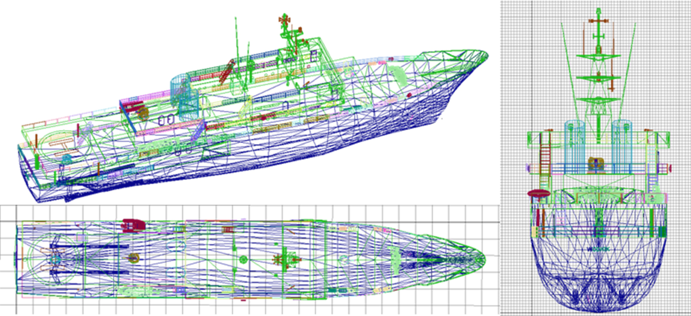
The process of generation of a three-dimensional model of a ship and in particular of its outline is relevant when it comes to the simulation of a mooring manoeuvre and when accounting for its geometry for the effects of ship-ship and ship-wharf interactions, etc. The first stage of the 3D model generation (for example, “3D Studio Max”) is the creation of the model construction grid (Figure 1). The sketches from the ship's technical documentation proved to be useful here.

Figure 1. Construction grid of a three-dimensional model of a vessel.

The next step is the overlaying of textures based on photographs, followed by rendering, which allows for a visualisation of the virtual model. The complete model is transformed to a format compatible with the simulator's environment (Figure 2).

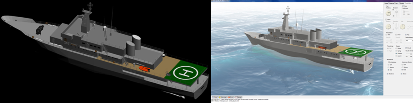
Figure 2. Model of a vessel after rendering.

2.1.2. Creation of the ship's motion

This involves the development of a simulation vessel based on input data with the use of the Virtual Shipyard application. This is the most important stage in the whole process of producing a virtual model of a ship. The process requires the introduction of a range of data and coefficients conditioning the model's credibility of behaviour in specific hydro-meteorological conditions. Generally, the process can be presented as shown in Figure 3.

Figure 3. Creating the model of a vessel's motion.

It is possible to devise simulation models using the data from the simulator's database, the technical documentation of a ship or the actual records. Therefore, for the purposes of the comparative analysis, two versions of the simulation model of ORP Wodnik were created:

1. (a) an “extended version” – based on detailed data from the ship's technical documentation;

2. (b) a “corrected version” – a corrected “extended version” based on the real manoeuvring data of the reference ship.

Each of the models mentioned above is characterised by a different degree of adequacy with comparison to the real-world model. Their limitations were confirmed by the method created for model assessment allowing for a determination of their suitability to various purposes. The results of this comparative analysis of both models in comparison with their reference ships are presented further in this article.

2.1.3. Basic manoeuvring tests

These allow for verification of the model's behaviour under specific weather conditions, or the performance of manoeuvres in accordance with IMO guidelines. During this process, the application shows all forces and coefficients available in the mathematical model of the simulation.

2.1.4. Creation of the ship's manoeuvring documentation

Alongside the creation of an object to be imported to the simulator's software, the ship's manoeuvring documentation in the form of three conventional documents is created: a pilot card, a wheelhouse poster, and a manoeuvring booklet.

2.1.5. Generation of the installation file

The process of creation of a simulation model ends with the generation of an output file that should be installed as a new object in the simulator environment. The algorithm of the construction process of a vessel's simulation model is presented in Figure 4.

Figure 4. Construction of a vessel's simulation model.

3. VESSEL SIMULATION MODEL - THE EVALUATION PROCESS

We decided to apply a multi-criteria analysis method to this problem. These methods are being used more and more frequently in various disciplines of science. Looking for a mathematical apparatus, we decided that the main goal must be the ability to apply a reference value, which will be the result of manoeuvring tests carried out on a real ship. Therefore, a multi-criteria evaluation method was chosen, as it utilises a reference of quality described among others in Jajuga and Walesiak (Reference Jajuga, Walesiak, Decker and Gaul2000), Cox and Cox (Reference Cox and Cox2000), Byun and Lee (Reference Byun and Lee2005) and Kläs et al. (Reference Kläs, Trendowicz, Lampasona and Münch2010).

The proposed method combines tools of various fields of knowledge such as: multi-criteria optimisation, multi-criteria decision support and statistical comparative analysis. The aim of the adopted method is to define the degree of correspondence of the selected vessel simulation model parameters with their real-world counterparts. This degree will be called “distance” $\lpar d_{U_{j}}\rpar $ and be defined as the difference of values of the parameters under study. In addition, the multi-criteria evaluation method enables several models to be analysed at the same time and their level of correspondence to be determined.

3.1. Defining the analysis goal and observation matrix of technical parameters

Owing to the significant number of technical parameters of a simulation model that can be tested, the goal of the comparative process must first be established. Depending on the goal, an adequate set of diagnostic parameters can be chosen, which will be subject to verification. The verification of a simulation model may be present only within a specific functional scope. It is possible, therefore, to select several research scenarios in which it is necessary to verify the individual parameters of the virtual model. Defining these scenarios will make it easier to choose an adequate set of technical parameters and, if necessary, apply weights to them, depending on their importance. In Table 1, the most frequently used sets of technical parameters suited to the research goal are shown.

Table 1. Example research scenarios and technical parameter features.

It may therefore be stated that for each of the simulation models studied, creating the set M = {M _i, i = 1, …, n}, may be defined by technical parameters (U _j) for j = 1, …, k. The technical parameters included by the authors are: drift speed, course over ground, drift angle, roll, pitch, etc. The distance of technical parameters of the simulation model from the real vessel affects the scope of its use in a scientific process. If the number of technical parameters k > 1, the evaluation of a model will be of a multi-criteria nature. Then, a set of technical parameters will be formed which will characterise the simulation model:

(1)$${\bi U} = \lcub U_1\comma \; U_2\comma \; \ldots\comma \; U_k\rcub $$

where U _j is the jth technical parameter describing the simulation model (j = 1, …, k) and k is the number of distinguished features.

After inserting the assumption Equation (1) into the function of the set of simulation models (M), a matrix of observations of technical parameters of individual models can be created:

(2)$${\bf U}_{{\bf M}} = \left[\matrix{U_1 \lpar M_1\rpar & U_1 \lpar M_2\rpar &\cdots & U_1 \lpar M_i\rpar \cr U_2 \lpar M_1\rpar & U_2 \lpar M_2\rpar &\cdots & U_2 \lpar M_i\rpar \cr \vdots &\vdots &\vdots &\vdots \cr U_j \lpar M_1\rpar & U_j \lpar M_2\rpar &\cdots & U_j \lpar M_i\rpar \cr }\right]$$

Likewise, a matrix of observations of technical parameters for the real vessel is created:

(3)$${\bf U}_{\bf W} = \left[\matrix{U_1 \lpar W\rpar \cr U_2 \lpar W\rpar \cr \vdots \cr U_j \lpar W\rpar \cr }\right]$$

During the measurements of technical parameters in comparable hydro-meteorological conditions, different values for individual parameters are obtained. Their number depends on the quantity of measurements made in real conditions. The larger the amount of data gathered in similar conditions, the more accurate the comparative analysis will be. Then, the elements of matrices U_M, U_W will be just arithmetic means of individual technical parameters from individual measurements.

3.2. Determination of the distance between the studied parameters and the real vessel

The distance between the individual technical parameters of the simulation model and the real vessel can be calculated using the formula:

(4)$$d_{U_j} = \sqrt{\sum_{j=1}^k w_{U_j} \lsqb U_j \lpar M_i\rpar - U_j \lpar W\rpar \rsqb ^2} $$

where $w_{U_{j}}$ is the weight for the jth technical parameter, U _j(M _i) is the normalised value of the jth technical parameter for the ith simulation model and U _j(W) is the normalised value of the technical parameter for the real vessel.

In this research problem, the most favourable situation is when distance (understood as the difference) between the individual technical parameters of the simulation model and the real vessel is as small as possible and is within the specified range:

(5)$$d_{U_j} = \left\{\matrix{d_{U_j}^0 & \quad \hbox{for} & d_{U_j} \in \langle a \comma \; b \rangle \cr d_{U_j} & \quad \hbox{for} &\hbox{other values} \cr}\right. $$

The values from the range $\langle a \comma \; b \rangle$ are the adopted limits of acceptability of the adequacy of the simulation model and are determined before each evaluation of the simulation models.

Depending on the type of research task defined in Table 1 with respect to which model M _i is to be used, the effect of the individual technical parameters on the degree of correspondence can be determined. For this purpose, the weight of an individual U _j should be determined in the studied model M _i. Weight may take values from the range $w_{U_{j}} \in \langle 0 \comma \; 1\rangle$.

In comparative practice, a quick assessment of the quality of determinations is related to the need to present the non-correspondence of a model with the real vessel as a percentage, therefore presenting the distance $d_{U_{j}}$ as a percentage seems reasonable. Then, the values obtained from Equation (4) can be specified as follows.

If U _j(M _i) > U _j(W) then:

(6)$$d_{U_j} \lpar \% \rpar = \displaystyle{{U_j \lpar M_i\rpar - U_j \lpar W\rpar } \over {U_j \lpar M_i\rpar }} \cdot 100\% $$

If U _j(M _i) < U _j(W) then:

(7)$$d_{U_j} \lpar \% \rpar = \displaystyle{{U_j \lpar M_i\rpar - U_j \lpar W\rpar }\over{U_j \lpar W\rpar }} \cdot 100\% $$

3.3. The use of the method of evaluation for a chosen research scenario

In order to verify the correctness of the assumptions, the authors adapted the assumed evaluation model to a research scenario: “The analysis of the effect of wind and waves on the behaviour of a drifting vessel” (Table 1). To this end, the technical parameters of the model subjected to assessment for accuracy were specified. A set of technical parameters takes the following form:

$${\bi U} = \lcub U_1\comma \; U_2\comma \; U_3\comma \; U_4\comma \; U_5\rcub $$

where U ₁ is the drift angle (difference of a change of a true course in the analysed time range) [^°], U ₂ is the drift speed (average drift speed in the analysed time range) [kn], U ₃ is the course over ground (average value in the analysed time range) [^°], U ₄ is the pitch (maximal pitch values) [^°] and U ₅ is the roll (maximal roll values) [^°].

Two versions of a simulation model of a ship were built, therefore, the set of simulation models will take the following form:

$${\bi M} = \lcub M_1\comma \; M_2\rcub $$

where M ₁ is the “extended” model and M ₂ is the “corrected” model.

According to Equation (2), a matrix of technical parameters in the function of models (U_M) was created, and according to Equation (3), a matrix of technical parameters of the reference (U_W) was built:

$${\bf U}_{{\bf M}} = \left[\matrix{U_1 \lpar M_1\rpar & U_1 \lpar M_2\rpar \cr U_2 \lpar M_1\rpar & U_2 \lpar M_2\rpar \cr U_3 \lpar M_1\rpar & U_3 \lpar M_2\rpar \cr U_4 \lpar M_1\rpar & U_4 \lpar M_2\rpar \cr U_5 \lpar M_1\rpar & U_5 \lpar M_2\rpar \cr }\right]\quad {\bf U}_{\bf W} = \left[\matrix{U_1 \lpar W\rpar \cr U_2 \lpar W\rpar \cr U_3 \lpar W\rpar \cr U_4 \lpar W\rpar \cr U_5 \lpar W\rpar \cr }\right]$$

Next, using Equations (4), (6) and (7), the distances for individual technical parameters were specified. In the research scenario, only the basic technical parameters are analysed, therefore, a constant value of weights $w_{U_{j}} = 1$ is assumed. Then, according to Equation (5), a correction of coefficients will follow. For the purpose of this article, we specified acceptability limits for the simulation model's adequacy as $d_{U_{j}} \in \langle -15\% \comma \; + 15\% \rangle$. A practical realisation of the method is presented next.

4. NUMERICAL TEST

A numerical test was performed with the use of a navigation and manoeuvring simulator located in the Polish Navy Academy in Gdynia. It was divided into two stages. The first consisted in verification of the level of correspondence of the “extended” model generated based on real construction parameters. The second stage involved checking the “corrected” model against the function of coefficients. A drifting vessel was subject to analysis (Table 1, scenario 3). Table 2 shows the actual records taken during the measurement session conducted on board ORP Wodnik (Czaplewski and Zwolan, Reference Czaplewski and Zwolan2016). These records provided the basis for the comparative analysis.

Table 2. Results of measurements for the vessel based on real-world studies.

¹True Wind Direction

²True Wind Speed

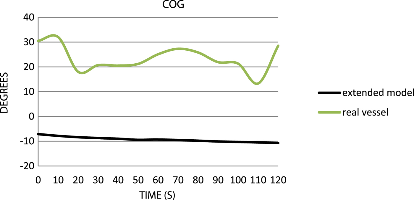
Table 3 presents the results of a simulation test of the “extended” model. The test was performed under simulated hydro-meteorological conditions corresponding to the real-world studies. Graphic results of comparative analysis of the “extended” model with the real vessel are presented in Figures 5–9.

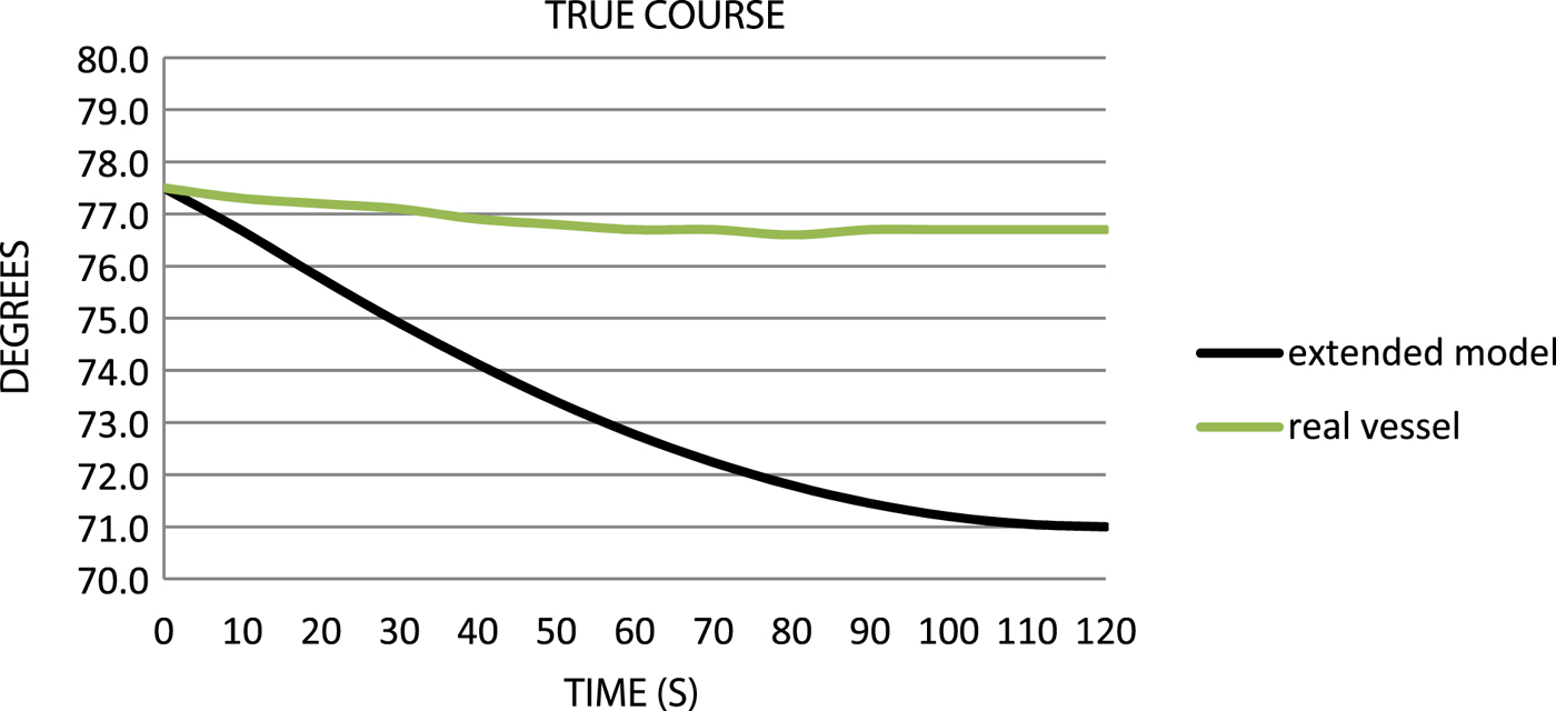
Figure 5. Comparison of the true courses.

Figure 6. Comparison of the courses over ground.

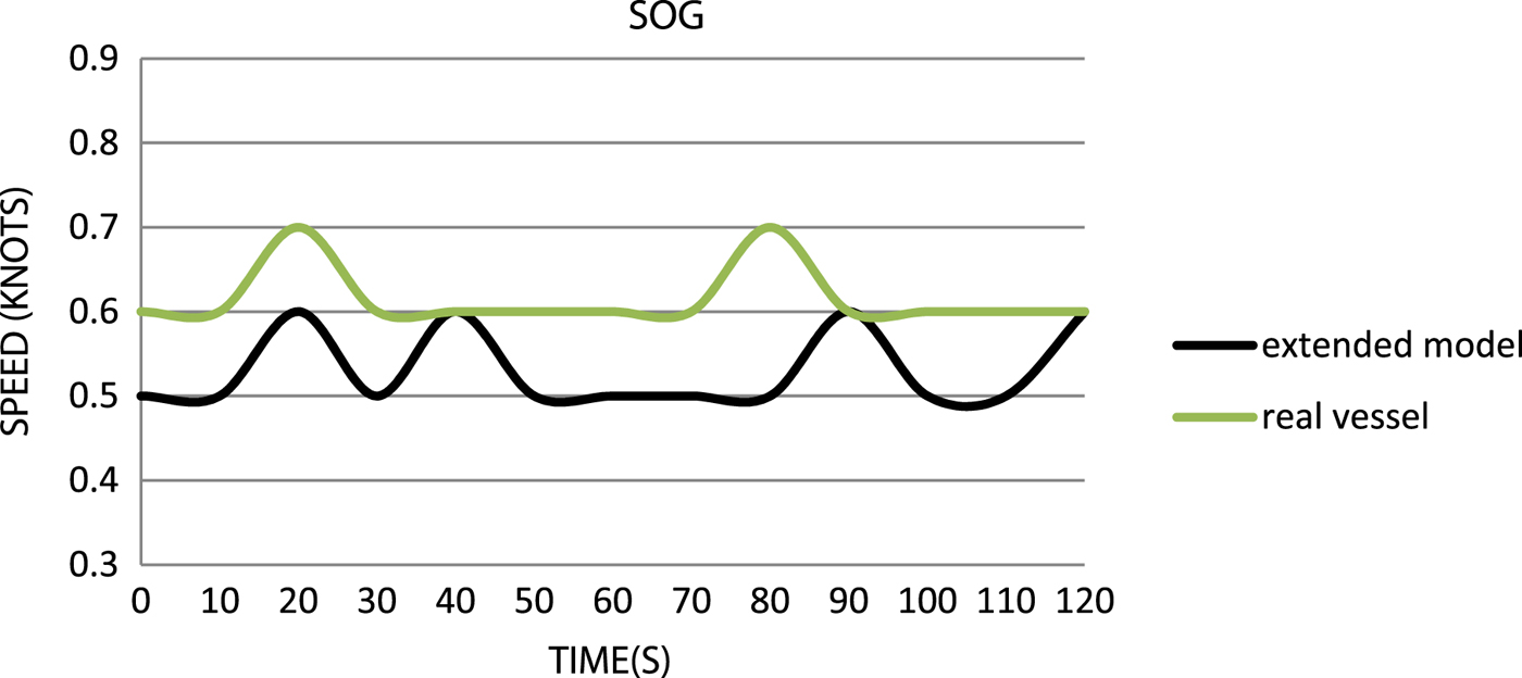
Figure 7. Comparison of the speeds over ground.

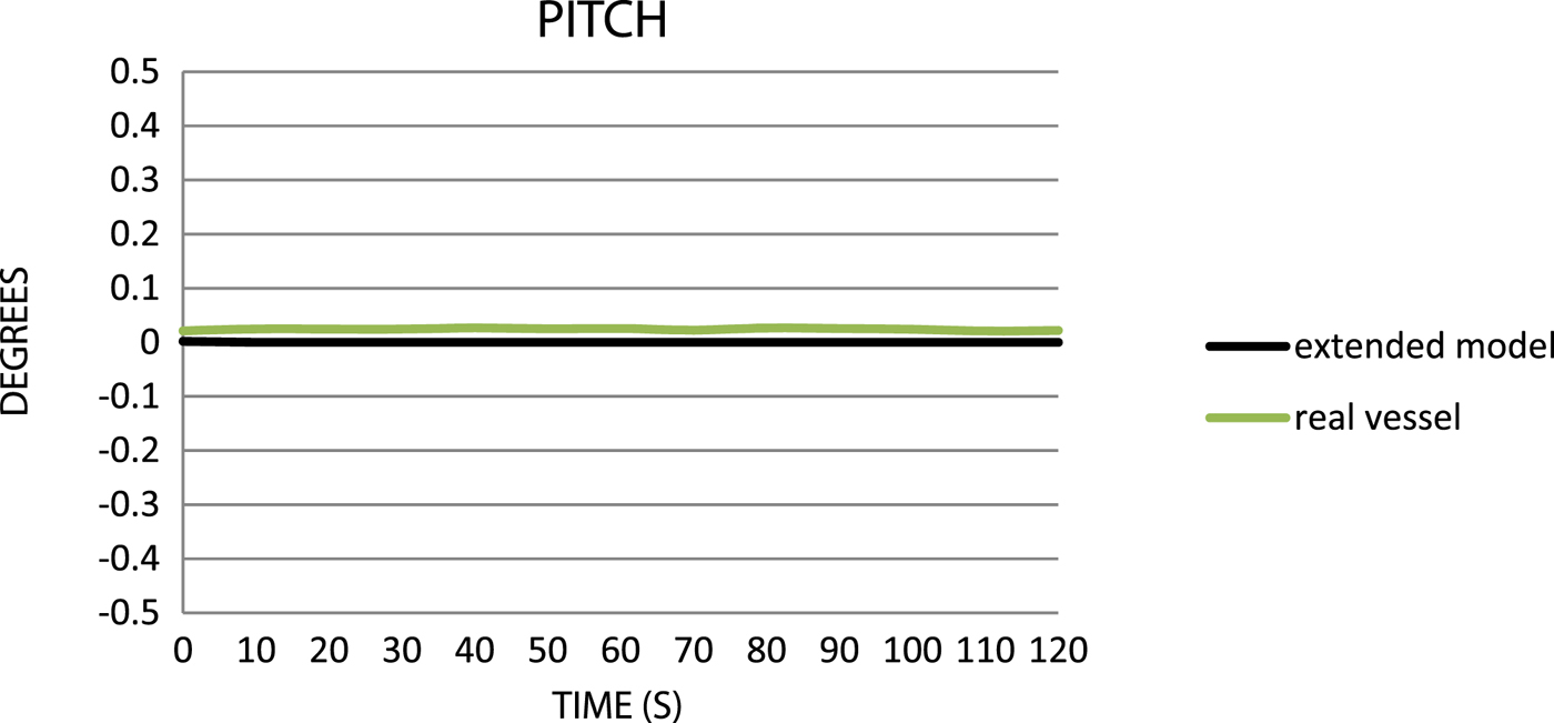
Figure 8. Comparison of the pitch values.

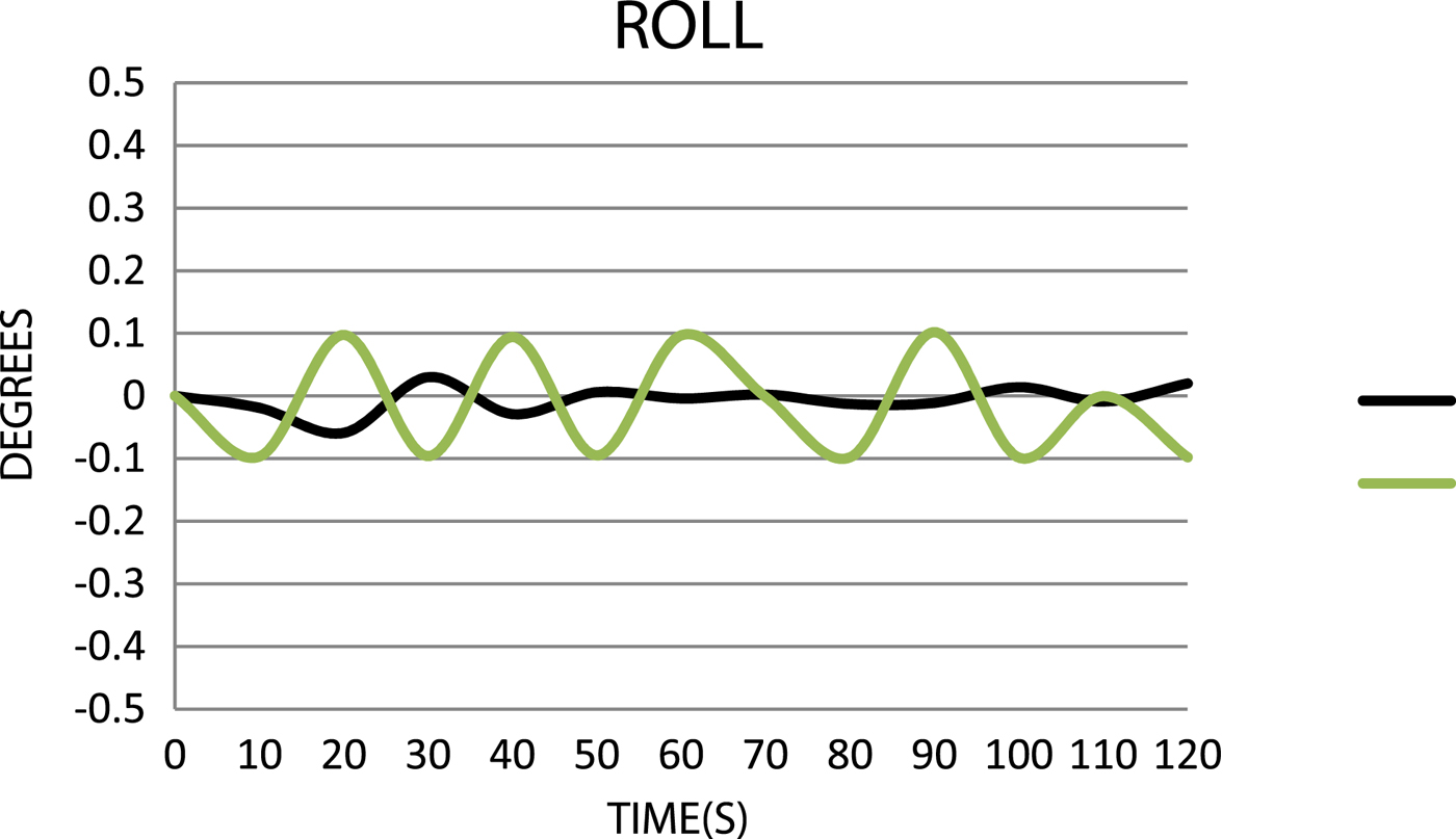
Figure 9. Comparison of the roll values.

Table 3. Results of the simulation test for the “extended” model.

As shown in Figure 5, the “extended” model changes its True Course (TC) under the influence of wind much more quickly. There is, however, a full compliance when it comes to the direction of the movement of the bow and stern.

The analysis of the track describing the Course Over Ground (COG) indicates significant differences between the two vessels; the difference is about 40^° (Figure 6). This illustrates a problem that despite the correct introduction of data pertaining to the lateral wind exposed area, the curves responsible for the drift angle need revising.

When comparing the drift speed data (Speed Over Ground, SOG) (Figure 7), it can be seen that the introduction to the model of detailed data concerning wind exposed areas or the underwater part of the hull does not give satisfactory results, and the simulation drifts more slowly than the real vessel.

For pitch and roll data, it is clear that the “extended” model is not correctly calibrated with the reference. Pitch is close to 0^° (Figure 8), which is caused by waves at transverse angles. The roll of the “extended” model is too small with respect to the reference (Figure 9), so the model also needs calibration in this respect.

According to the methodology of the model assessment described in this paper, the values of the technical parameters were specified for the real vessel, “extended” model (Table 4) and the “corrected model” (Table 7).

Table 4. Technical parameters of the extended model and the real vessel.

For the parameters presented in Table 4, a matrix of the “real vessel” technical parameters is constructed:

$${\bf U}_{\bf W} = \left[\matrix{U_1 \lpar W\rpar \cr U_2 \lpar W\rpar \cr U_3 \lpar W\rpar \cr U_4 \lpar W\rpar \cr U_5 \lpar W\rpar \cr }\right]= \left[\matrix{-0{\cdot}800 \cr 0{\cdot}620 \cr 23{\cdot}500 \cr 0{\cdot}007 \cr 0{\cdot}200 \cr }\right]$$

Also constructed is the matrix of the “extended” model's technical parameters:

$${\bf U}_{{\bf M}} = \left[\matrix{U_1 \lpar M_1\rpar \cr U_2 \lpar M_1\rpar \cr U_3 \lpar M_1\rpar \cr U_4 \lpar M_1\rpar \cr U_5 \lpar M_1\rpar \cr }\right]= \left[\matrix{-6{\cdot}500 \cr 0{\cdot}530 \cr 9{\cdot}800 \cr 0{\cdot}002 \cr 0{\cdot}089 \cr }\right]$$

The matrix of distances of the technical parameters du calculated based on Equation (4) takes the following form:

$${\bf du} = \left[\matrix{d_{U_1} \lpar M_1\rpar \cr d_{U_2} \lpar M_1\rpar \cr d_{U_3} \lpar M_1\rpar \cr d_{U_4} \lpar M_1\rpar \cr d_{U_5} \lpar M_1\rpar \cr }\right]= \left[\matrix{5{\cdot}700 \cr 0{\cdot}090 \cr 0{\cdot}110 \cr 0{\cdot}005 \cr 0{\cdot}111 \cr }\right]$$

The calculated percentage values of non-correspondence of distances $\lpar d_{U_{j}}\rpar $ for the specific technical parameters of the “extended” model with respect to the reference are shown in Table 5.

Table 5. Percentage values of non-correspondence of distances for individual technical parameters of the “extended” model with respect to the real vessel.

Based on the analysis of the data included in the table it may be stated that the model created based on the real vessel's construction data did not meet the condition of the percentage tolerance for correspondence. Therefore, the coefficients of the “extended” model need to be corrected. Table 6 shows the results of the simulation tests in the “corrected” model. Graphic results of comparative analysis of the “corrected” model with the real vessel are presented in Figures 10–14.

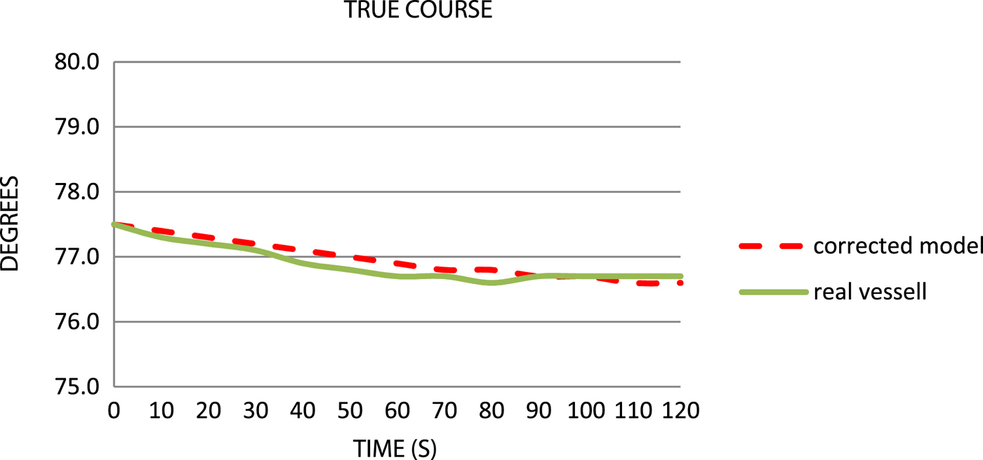
Figure 10. Comparison of the true courses.

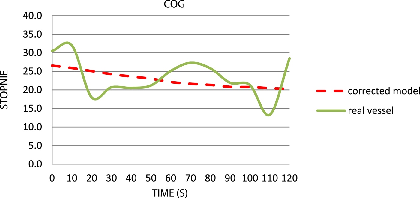
Figure 11. Comparison of the courses over ground.

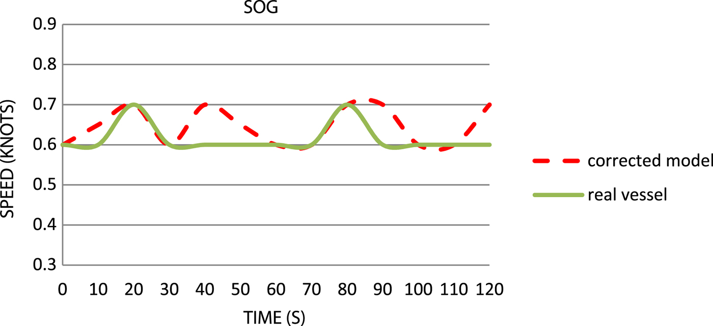
Figure 12. Comparison of the speeds over ground.

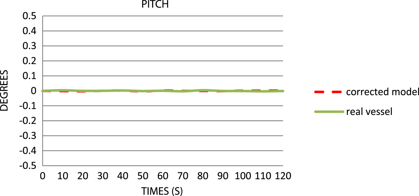
Figure 13. Comparison of the pitch values.

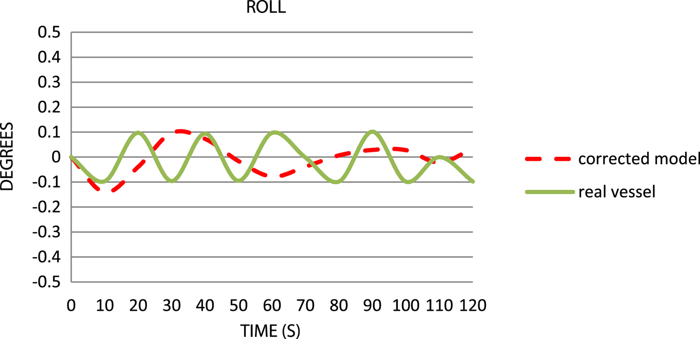
Figure 14. Comparison of the roll values.

Table 6. Results of simulation test for the “corrected” model.

It may be concluded from the above figure that differences of TC reach 0 · 1^°–0 · 2^° after 2 minutes (Figure 10). A noticeable difference, however, is a steadier movement of the simulation model.

The difference when comparing the mean values of the COG (Figure 11) of both vessels and the angle between the starting and the final position resulting from the adjustment of the model's coefficients is less than 1^°.

The comparative charts showing the values of SOG (Figure 12) indicate that accuracy with the real vessel occurs for the average speed. However, what is noticeable is a different reaction of the real vessel's hull from that of the simulation model with regard to the time ranges of differences in drift speeds. Most importantly, however, the average drift speed is fully correspondent with the ship.

The pitches (Figure 13) are close to 0^°, which is induced by waves at transverse angles. The roll (Figure 14) for a drifting vessel, with a sea state one, does not exceed 0 · 2^°. A remarkable improvement can be seen in the case of the model's behaviour in this aspect as compared with the “extended” model. The chart shows only maximum roll in the selected time ranges. To obtain a more precise analysis of roll, the time ranges must be much smaller.

The matrix of observations of technical parameters for the real vessel is the same as it was during the analysis of the “extended” model. The matrix of the observations of technical parameters for the “corrected” model, however, takes the following form:

$${\bf U}_{{\bf M}} = \left[\matrix{U_1 \lpar M_2\rpar \cr U_2 \lpar M_2\rpar \cr U_3 \lpar M_2\rpar \cr U_4 \lpar M_2\rpar \cr U_5 \lpar M_2\rpar \cr }\right]= \left[\matrix{-0{\cdot}900 \cr 0{\cdot}650 \cr 22{\cdot}700 \cr 0{\cdot}006 \cr 0{\cdot}238 \cr }\right]$$

The matrix of distances of technical parameters du is as follows:

$${\bf du} = \left[\matrix{d_{U_1} \lpar M_1\rpar \cr d_{U_2} \lpar M_1\rpar \cr d_{U_3} \lpar M_1\rpar \cr d_{U_4} \lpar M_1\rpar \cr d_{U_5} \lpar M_1\rpar \cr }\right]= \left[\matrix{0{\cdot}100 \cr 0{\cdot}030 \cr 0{\cdot}800 \cr 0{\cdot}001 \cr 0{\cdot}038 \cr }\right]$$

Having analysed the data contained in Table 8 concerning the final comparative analysis, it may be asserted that the non-correspondence values of the “corrected” model's technical parameters with respect to the real vessel, for four out of five parameters under study, is contained within a specific percentage range. Only the heel values exceed the assumed acceptability limits. This is because the angle values of heels are minute as the analysis is performed at sea states equal to one and two. Therefore, the differences equal to decimal numbers of an angle translate into significant percentage differences. Final results show that the model created based on construction data grossly deviates from the real vessel. Its application in a research process and the given scenario would result in significant errors in the interpretation of the studies. However, the adjustment of the model's coefficients significantly improves the degree of the models' correspondence with the real vessel.

Table 7. Values of technical parameters of the “corrected” model and the real vessel.

Table 8. Percentage values of distance non-correspondence of the “corrected model's” individual technical parameters with respect to the real vessel.