


1. Introduction
Unsteady flow conditions occur in a variety of applications, such as helicopters, wind turbines and biological locomotion. Here, the forces and moments on an airfoil are considered as its angle of attack is varied in time. For attached flows, the deviations of aerodynamic loads due to dynamic changes in the angle of attack are small and the magnitudes are comparable to those in static conditions (McCroskey & Pucci Reference McCroskey and Pucci1982). In the attached, linear, part of the lift curve, the unsteady load fluctuations can be analytically described and reasonably well predicted from theories by Theodorsen (Reference Theodorsen1935) and von Kármán & Sears (Reference von Kármán and Sears1938). As these theories are based on a flat plate subject to small amplitude oscillations in potential flow, they become inaccurate once the flow separates. Dynamic flow separation on an airfoil typically occurs at or above the static stall angle of the airfoil, which depends on the Reynolds number of the flow, the airfoil shape, turbulence levels and surface roughness, among other factors. When the static stall angle is rapidly exceeded in unsteady pitching manoeuvres, flow separation can be delayed, such that higher angles are required for stall. This can cause unsteady aerodynamic loads to exceed static loads many times over. Such events may result in structural damage to the machinery or loss of control in situations where stall is relied upon. For this reason, considerable effort has been made since the 1970s to characterize the mechanisms and flow behaviour of dynamic stall (Carta Reference Carta1974; Carr, McAlister & McCroskey Reference Carr, McAlister and McCroskey1977; McAlister, Carr & McCroskey Reference McAlister, Carr and McCroskey1978; McCroskey et al. Reference McCroskey, McAlister, Carr and Pucci1982). The majority of these efforts have been focused on the investigation of periodic oscillations of an airfoil (McCroskey Reference McCroskey1982), where the motion path is characterized by a pitching, heaving or translating motion, or any combination thereof. Inherently, a periodic oscillation results in the overlapping of two fundamentally different processes which occur within a single pitching period, namely the separation and the subsequent reattachment of the boundary layer. Depending on the kinematics and the time scales of the oscillation, these processes can be more or less entangled and therefore become difficult to analyse.
For this reason, the aim of the present study is to investigate the effects of dynamic flow separation separately from those of dynamic reattachment. To do so, well-prescribed kinematics corresponding to ramp type motions are investigated. In order to better compare the results from the individual pitching manoeuvres with those of continuous oscillations, the paths of the ramp motions were of sinusoidal form. The time dependence of the angle of attack and thus the pitching motion was defined by
 \begin{equation} \alpha(t) = \begin{cases} \bar{\alpha} - \hat{\alpha}, & t < 0, \\ \bar{\alpha} + \hat{\alpha} \sin\left(2 {\rm \pi}f t - {\rm \pi}/2\right), & 0 \leq t \leq \dfrac{1}{2f},\\ \bar{\alpha} + \hat{\alpha}, & t > \dfrac{1}{2f}, \end{cases} \end{equation}
where  $\bar {\alpha }$ depicts the mean angle,
  $\hat {\alpha }$ is the mean-to-peak amplitude,
  $f$ is the pitching frequency in Hz and
  $t$ is the dimensional time in s. The restricted domain was chosen such that the pitching frequencies between ramps and continuous pitching are directly comparable. As a result, the pitching motions begin at
  $t = 0$ and end at
  $t = 0.5 f^{-1} = T/2$. For the remainder of this study, the pitching motions are referred to as sinusoidal half-cycles or ramps.
Apart from the geometric characteristics of the pitching motion, the remaining parameters which govern the problem of unsteady pitching manoeuvres are the Reynolds number  $Re$, the Mach number
  $Ma$ and the reduced frequency
  $k$. A distinguishing feature of the present study is the wide parameter space covered, enabled by a unique highly pressurized wind tunnel, in which the experiments were performed. This facility allowed the investigation to be performed at high Reynolds numbers
  $Re_c = \rho U c / \mu$, where
  $c$ is the airfoil chord,
  $\rho$ is the fluid density,
  $U$ is free-stream velocity and
  $\mu$ is the dynamic viscosity. Since the high Reynolds numbers are achieved by increasing the density, the velocities can be kept low (
 ${<}4.5\,{\rm m}\,{\rm s}^{-1}$ for all test cases), enabling tests at very low Mach numbers
  $Ma = U / a \leq 0.013$, where
  $a$ is the speed of sound. Compressibility effects, which have a considerable impact on the dynamic stall process as elucidated by Carr (Reference Carr1988), can thus be neglected. Furthermore, the low velocity implies that the time scales can be kept relatively large, enabling highly dynamic events to be studied at high Reynolds numbers, something that is extremely challenging in conventional facilities.
To allow for convenient comparisons with continuous oscillations, the unsteadiness is expressed as the reduced frequency  $k$, instead of the reduced pitch rate
  $r$, which is commonly used for linear ramp profiles. The reduced frequency
  $k = \omega b / U$ is based on the half-chord length
  $b = c/2$ as the convective length scale and the angular velocity
  $\omega = 2 {\rm \pi}f$. As such, there are two time scales that are relevant to the unsteady flow field: the convective time scale of the flow, which non-dimensionalizes time as
  $t^* = t U / c$, and the time duration of the pitching motion, which non-dimensionalizes time as
  $\tilde {t}=t\omega /{2{\rm \pi} }$. The ratio of these two non-dimensionalized times yields the reduced frequency as
  $\tilde {t} / t^*=k/{\rm \pi}$.
In order to compare the results from this paper with other studies on ramp motions in the literature characterized by a reduced pitch rate  $r = \dot {\alpha } c / U_{\infty }$, a reduced pitch rate
  $r_{lin}$ can be calculated by a linear approximation of the sinusoidal half-cycle. Accordingly, the angular pitch rate is
  $\dot {\alpha } = 4 \hat {\alpha }f$. As a result, the linear reduced pitch rate can be related to the reduced frequency given in the figures by
  $r_{lin} = 4k\hat \alpha / {\rm \pi}$.
Likely due to the focus on helicopter aerodynamics and the use of relatively thin airfoils on helicopters, many early and highly influential studies on unsteady airfoil experiments link the occurrence of dynamic stall inevitably to a vortex structure emerging from the leading-edge region (Carr et al. Reference Carr, McAlister and McCroskey1977; McAlister et al. Reference McAlister, Carr and McCroskey1978; McCroskey Reference McCroskey1982). Comparable remarks can be found in more recent publications as well (Simão Ferreira et al. Reference Simão Ferreira, Van Kuik, Van Bussel and Scarano2009; Gupta & Ansell Reference Gupta and Ansell2019). Similarly, the description of unsteady insect and bird flight is generally associated with a leading-edge vortex (Dickinson, Lehmann & Sane Reference Dickinson, Lehmann and Sane1999; Lentink Reference Lentink2013). It is important to note that these descriptions concern the dynamic stall process at specific operating conditions, which cannot be generalized for arbitrary wing shapes or Reynolds numbers.
Only a few previous studies, such as McCroskey et al. (Reference McCroskey, McAlister, Carr, Pucci, Lambert and Indergrand1981) and Gracey, Niven & Galbraith (Reference Gracey, Niven and Galbraith1989), in which multiple airfoils were studied, note that the emergence of the vortical structure is not necessarily bound to the leading edge, but may arise much further aft on the airfoil. This appears to be particularly true for thicker airfoils, for which the leading-edge region remains attached throughout the stall process, while the mid-chord to trailing-edge region of the airfoil experiences highly disturbed and separated flow which eventually rolls up into a vortical structure.
The isolated effect of airfoil thickness was investigated in a numerical study by Sharma & Visbal (Reference Sharma and Visbal2019), who found that the transient aerodynamics differs considerably between the tested airfoils at a Reynolds number of  $Re_c = 200\,000$. The same authors noted that with increasing airfoil thickness the mechanism of stall onset changes and the size of the laminar separation bubble (LSB) decreases. The stall process on thinner airfoils is triggered by the pressure-gradient-induced bursting of the LSB close to the leading edge, whereas thicker airfoils display a gradual trailing-edge separation which moves upstream up to the LSB. In the latter case, it was not certain whether the approaching separation causes a collapse of the LSB or the separation itself triggers the onset of the stall. In a numerical study by Benton & Visbal (Reference Benton and Visbal2019) at a higher Reynolds number of
  $Re_c = 1.0 \times 10^6$, the same mechanism of augmented trailing-edge separation was found to penetrate the LSB, which initiated the vortex formation and the stall process. In comparison with previous studies, the authors concluded that the upstream progression of the trailing-edge separation intensifies with Reynolds number.
Similarly to static stall behaviour, dynamic stall can be categorized into three types of stall, namely leading-edge stall, trailing-edge stall and mixed stall according to McCroskey et al. (Reference McCroskey, McAlister, Carr, Pucci, Lambert and Indergrand1981), who tested six different airfoil geometries in a large parameter study. Quasi-static behaviour was found not to be a reliable guide for dynamic performance, as large differences between the different airfoil models were observed. Furthermore, boundary layer separation characteristics were found to be additionally dependent on the reduced frequency for some of the tested airfoils.
A characteristic, widely described feature of dynamic stall is delayed boundary layer separation, which eventually forms a larger-scale vortical structure that can momentarily increase lift before the airfoil ultimately stalls. In steady flows, the point of flow reversal and the point of initial boundary layer separation are identical. The criterion for separation was formulated by Prandtl as  $\partial u/\partial y = 0$ at
  $y= 0$. However, in unsteady boundary layers flow reversal and separation generally do not coincide (Koromilas & Telionis Reference Koromilas and Telionis1980). Instead, in the case of pitching airfoils a thin layer of reversed flow momentarily appears at the bottom of the boundary layer prior to the probable but not necessary onset of separation. This thin layer generally does not affect the outer extent of the boundary layer. As a result, the inviscid flow field and thus the surface-pressure distribution remain largely unaltered (Gracey et al. Reference Gracey, Niven and Galbraith1989).
2. Experimental set-up
The experiments were conducted in the High Reynolds number Test Facility (HRTF), a closed-loop high-pressure wind tunnel located at the Gas Dynamics Laboratory at Princeton University. The flow facility, which is shown in figure 1, uses dry air as a working fluid, compressed to static pressures of up to  $p_0 = 24$ MPa (3500 psi or 238 bar). For all test cases, density and viscosity were calculated from static pressure and temperature measurements by employing the real-gas relationship
  $\rho = p_0 / (zRT)$, where
  $\rho$ is the fluid density,
  $R$ is the specific gas constant for air,
  $T$ is the temperature and
  $z$ is the compressibility factor. The exact procedure is outlined in Zagarola (Reference Zagarola1996) and Miller et al. (Reference Miller, Duvvuri, Brownstein, Lee, Dabiri and Hultmark2018).

Figure 1. The High Reynolds number Test Facility (HRTF) located at the Princeton Gas Dynamics laboratory. (a) Connection to the external motor which drives the pump; (b) flow conditioning and subsequent contraction; (c) access port and model location as shown in figure 2 highlighted in red.
The flow is conditioned by a coarse-meshed grid, a honeycomb grid and a fine grid before it passes through a  $2.2:1$ nozzle into the circular test section. Depending on the Reynolds number, the flow conditioning yields turbulence intensity levels between
  $0.3\,\%$ and
  $1.1\,\%$ (Jiménez, Hultmark & Smits Reference Jiménez, Hultmark and Smits2010). Independently of the tunnel static pressure, a free-stream velocity of up to
  $10\,{\rm m}\,{\rm s}^{-1}$ can be attained in the test section, which measures 0.49 m in diameter and 4.88 m in length. The model is supported in an access port located 1.1 m downstream of the entrance to the test section. Further information on the facility can be found in Jiménez et al. (Reference Jiménez, Hultmark and Smits2010), Miller et al. (Reference Miller, Duvvuri, Brownstein, Lee, Dabiri and Hultmark2018) and Miller et al. (Reference Miller, Kiefer, Westergaard, Hansen and Hultmark2019).
2.1. Airfoil model
A NACA0021 airfoil profile with a chord length of  $c = 0.17$ m and an aspect ratio of
  $AR = 1.5$ was employed in the experiments. The thickness of 21 % was chosen to make the study relevant to modern day wind turbines, where the thinnest part of the blade is commonly of the order of 20 %. The relatively low aspect ratio was chosen due to a combination of spatial constraints, Reynolds number and angular velocity requirements. To reduce end effects, the model was equipped with elliptical endplates, as shown in figure 2. As detailed in Brunner et al. (Reference Brunner, Kiefer, Hansen and Hultmark2021), the low aspect ratio delays stall to higher angles of attack in this experimental set-up. Furthermore, Angulo & Ansell (Reference Angulo and Ansell2019) found that a decrease in aspect ratio can lead to less severe dynamic stall.

Figure 2. Cutaway drawing of the airfoil assembly installed in an access port of the HRTF shown in figure 1. The annotations show the following components: (a) support plate; (b) load cell; (c) rotary table with attached stepper motor and encoder; (d) support rod; (e) endplates; ( f) airfoil model; (g) test section. Flow goes from left to right.
A total of 33 brass pressure taps were press fitted into the model, of which 32 were used for the tests. The assembly was sanded and polished by hand to a mirror-like finish, with a normalized root-mean-square roughness height,  $\kappa$, of
  $1.8 \times 10^{-7} \leq \kappa /c \leq 5.3 \times 10^{-7}$. The airfoil assembly was attached to a rotary stage using a circular support rod. The rotation axis was located at half-chord, which is different from many previous studies on dynamic stall. A downstream shift in the rotation axis has been found to cause a delay of dynamic stall to higher angles of attack (Helin & Walker Reference Helin and Walker1985). The combined frontal-area blockage of airfoil, endplates and support rod varies within
  $8\,\% \leq B \leq 15\,\%$ for angles of attack in the range of
  $0^{\circ } \leq \alpha \leq 40^{\circ }$. The airfoil surface was untripped to promote free transition of the airfoil boundary layer. A thorough description of the set-up can be found in Brunner et al. (Reference Brunner, Kiefer, Hansen and Hultmark2021).
2.2. Instrumentation
The data presented in this paper were derived from surface-pressure measurements acquired by 32 temperature-compensated differential pressure sensors (Honeywell Inc., model HSC). For comparison, forces and moments acting on the entire airfoil assembly were simultaneously acquired by a six-degrees-of-freedom force-torque sensor (JR3 Inc.) with a range of  ${\pm }200$ N and
  ${\pm }25$ N m. Force sensor and integrated pressure data showed excellent temporal agreement (see Appendix A.1), as well as nearly identical lift values. The use of independent pressure sensors allowed for increased accuracy as the individual sensor ranges could be chosen to match the anticipated pressures at their specific locations on the airfoil. Three transducer sensing ranges were used:
  ${\pm }$10 kPa for the highest anticipated pressures in the leading-edge region,
  ${\pm }$6.9 kPa for the intermediate range and
  $\pm$2.5 kPa for the smallest range. The pressure sensors, together with four 8-channel multiplexers for sampling, were embedded in a circuit board, which was mounted inside the airfoil model to ensure the shortest possible tube lengths between taps and sensors. A Pitot-static probe served as the reference pressure and was installed 2.24 chord lengths upstream of the airfoil. The free-stream velocity was measured by another Pitot-static probe located 4.35 chord lengths upstream of the airfoil rotation axis. The Pitot-static tube was connected to a Validyne DP-15 differential pressure transducer with a range of
  ${\pm }13.79$ kPa.
The angle of attack change around the rotation axis at half-chord was executed by a stepper motor connected to a rotary stage. The motion of the motor was hardware controlled by an external waveform generator, triggered by the data acquisition program. The angle of attack was monitored using a CUI AMT103 capacitive encoder attached to the stepper motor drive shaft.
This motion control, as opposed to the use of a lever mechanism to produce the angle variation, provided a high degree of freedom in the design of the waveform, so that not only sinusoidal but any arbitrary oscillations could be generated (Kiefer et al. Reference Kiefer, Brunner, Hultmark and Hansen2020). The set-up, however, was limited by the torque provided by the stepper motor to overcome the aerodynamic moment induced in a given test condition. This hardware limitation defined the envelope of the parametric study.
2.3. Data acquisition and test procedure
For a given test run, standstill zero readings were acquired before and after the experiment and their average was subtracted from the experimental data. In a second step, the airfoil was pitched in a no-flow condition to capture possible acceleration effects on the sensor readings due to the airfoil motion. The pressure sensors were not influenced by the motion itself, whereas force sensor data showed deviations from the standstill zero readings due to the inertia of the airfoil assembly. For every individual ramp motion, the flow field was allowed to equilibrate at the initial angle of attack before data acquisition commenced. The encoder and force sensor readings were carefully monitored to ensure there was no drift in the airfoil motion.
In all test cases, 50 pressure distributions were recorded during every half-cycle. The temporal bin averaging of the airfoil surface-pressure sensors showed no relevant loss in detail compared with the continuously acquired signals from the force sensor. A Savitzky–Golay filter, with a window size of  $\Delta t^* = 2.8$, was applied to all pressure data, from which lift, drag and moment data were then derived. The window size was carefully chosen to remove electrical noise but to retain all aerodynamic features of the time series. The data presented herein are the phase-averaged results of 150 individual half-cycles for any given test case.
The data were not corrected for blockage effects, aspect ratio, induction from the wake or the presence of endplates. Hence, the angle of attack  $\alpha$ is the geometric angle of attack. Corrections were applied to static data from this set-up in Brunner et al. (Reference Brunner, Kiefer, Hansen and Hultmark2021), which showed good agreement with data from previous literature.
3. Non-dimensionalization
A unique aspect of testing in a pressurized wind tunnel is that a test case, at a specific Reynolds number and reduced frequency, can be obtained using a variety of density–velocity combinations, even if the test model remains the same. Figure 3 shows an example of this for the case at  $Re_c = 3.0 \times 10^6$ and
  $k = 0.1$, where the data on the left-hand side of the figure are given in dimensional form and the right-hand side shows the non-dimensional lift
  $C_l$, drag
  $C_d$ and moment coefficient
  $C_{m,c/4}$ for the same three data sets, defined by
 \begin{equation} C_l = \frac{l}{\dfrac{1}{2} \rho U^2 c},\quad C_d = \frac{d}{\dfrac{1}{2}\rho U^2 c},\quad C_{m,c/4} = \frac{m_{c/4}}{\dfrac{1}{2} \rho U^2 c^2}. \end{equation}
Different combinations of velocity and density yield different dimensional forces and moments (panels  $b$–
$b$– $d$) because forces and moments scale linearly with density but quadratically with velocity (3.1a–c) for a given Reynolds number. The temporal differences in the dimensional data sets are caused by the linear relationship of velocity and dimensional pitching frequency in the reduced frequency. Panels (
 $e$–
$e$– $h$) convincingly show that both the magnitudes and the temporal developments collapse as a result of non-dimensionalization, as expected. The light-grey areas in this and all following figures highlight the period of airfoil motion. The variations from the phase-averaged means by two standard deviations (
 $2\sigma$) are indicated as shaded regions in panels (
 $b$–
$b$– $d$) and (
 $f$–
$f$– $h$). The non-dimensionalized standard deviations differ slightly from each other and are the smallest in the case of the highest velocity
  $U_\infty = 3.8\,{\rm m}\,{\rm s}^{-1}$, and thus the highest dimensional forces, which is expected as the instrumentation accuracy is increased at higher loads. The data for this study were acquired at static tunnel pressures in the range of
  $14.3 \leq p_0 \leq 216.8$ bar and free-stream velocities in the range
  $1.7 \leq U_\infty \leq 4.5\,{\rm m}\,{\rm s}^{-1}$. The flow conditions for all test cases are given in table 1 in Appendix B.

Figure 3. Lift, drag and pitching moment in dimensional form (left column) and non-dimensional form (right-hand column) for a pitch-up manoeuvre characterized by  $\bar {\alpha } = 24^\circ$,
  $\hat \alpha = 5^\circ$ and
  $k = 0.1$ at a Reynolds number of
  $Re_c = 3.0 \times 10^6$. Data sets were taken at different static pressures and velocities as specified in the legend.
4. Dynamic stall evolution
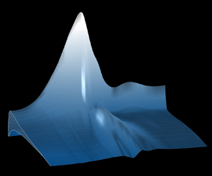
The temporal development of the suction-side pressure distribution of the baseline test case previously presented in figure 3 is shown in figure 4. Here,  $C_p$-levels are indicated by black isolines in increments of
  $\Delta C_p = 0.25$. Furthermore, vertical black solid lines mark start and end of the pitching manoeuvre and the black dashed line indicates the passing of the static stall angle. The origin
  $t = 0$, and therefore also
  $t^* = 0$, is defined as the beginning of the motion. During the pitching manoeuvre, the contour lines indicate a growing suction peak near the leading edge and a suction hump at half-chord and
  $t^* \approx 19$, which likely indicates the presence of a dynamic stall vortex (DSV) that causes peaks in the drag and moment histories (cf. figure 3). After the DSV has been convected downstream, a diminished suction peak remains at the leading edge, whereas the remainder of the airfoil suction side experiences a nearly constant pressure indicating a fully separated boundary layer downstream of
  $x/c > 0.15$.

Figure 4. Temporal development of the suction-side pressure distribution for the test case shown in figure 3:  $k = 0.1$,
  $\bar {\alpha } = 24^\circ$,
  $\hat {\alpha } = 5^\circ$,
  $Re_c = 3.0 \times 10^6$ and
  $Ma_\infty = 0.007$. The time span of
  $0 \leq t^* \leq 15.7$ indicates when the airfoil is in motion. Isolines indicate constant
  $C_p$-levels with values provided on the left-hand side of the plot.
Since specific  $C_p$-values have only a limited significance in transient manoeuvres, the plot is additionally coloured to illustrate the temporal change of the pressure distribution
  $\partial C_p / \partial t^*$, which results in a distinct picture of the pressure variations across the airfoil suction side. Here, blue colours reveal an increase in suction and red colours a loss of suction over time.
During the first half of the pitching motion, suction builds up across the entirety of the airfoil suction side with the strongest increase concentrated near the leading edge. With the passage of the static stall angle a region of suction loss (red) begins to develop at about half-chord and progresses toward the leading edge during the remainder of the pitching motion. During the same time, the trailing-edge region experiences a gradual increase in suction (blue) which advances forward up to  $x/c \approx 0.2$. Thus, all temporal pressure variations up until the formation of the DSV progress forward toward the leading edge, suggesting a stall type characterized by a gradual trailing-edge stall. Based on comparisons with other dynamic stall descriptions, such as Sharma & Visbal (Reference Sharma and Visbal2019), the suction increase near the trailing edge may stem from a roll-up of the separated shear layer.
The origin of the DSV appears to be located approximately at mid-chord, similar to findings reported in Mulleners & Raffel (Reference Mulleners and Raffel2012), Gupta & Ansell (Reference Gupta and Ansell2019) and Sharma & Visbal (Reference Sharma and Visbal2019). Benton & Visbal (Reference Benton and Visbal2019) describe the formation of the main DSV as the merging of two preceding vortices; a compact leading-edge vortex and a large, diffuse shear layer vortex. From the surface pressure data alone, it is not clear whether the same mechanisms dominate the stall process in the present experiments or only a single DSV develops. Following rapid convection of the DSV, brief surges of suction appear at the trailing edge (TE) and subsequently at the leading edge (LE). The surges imply alternating vortex shedding from TE and LE, where the LE vortex appears to convect downstream above the separated shear layer, as only minimal pressure traces of the vortex are visible in the region of separated flow downstream of  $x/c \approx 0.15$.
The characteristic picture of a growing region of suction increase (blue triangle shape) originating from the TE and enclosed by regions of suction loss in figure 4 is similarly prevalent throughout the vast majority of test cases presented herein. Thus, it is concluded that all test cases exhibit a nearly identical TE stall behaviour with minor differences induced by the variation of the four isolated test parameters. Relevant differences and similarities are elucidated in the following and are highlighted by the suction-side pressure variations of selected test cases shown in figure 5.

Figure 5. The temporal change of suction-side surface pressure presented for selected test cases (in bold numbers; see table 1 in Appendix B) of the Reynolds number ( $a$–
$a$– $c$), the mean angle (
 $d$–
$d$– $f$), amplitude (
 $g$–
$g$– $i$) and reduced frequency series (
 $j$–
$j$– $l$), respectively. Blue colours illustrate an increase in suction over time; red colours indicate a loss of suction. Black solid lines mark the start and end of the pitching motion; black dotted lines specify the passage of the static stall angle. Grey dotted horizontal lines mark the location of pressure taps.
4.1. Reynolds number
Figure 5(a,b,c) shows three test cases of the Reynolds number variation at  $Re_c = 0.5 \times 10^6$ (figure 5a),
  $Re_c = 2.0 \times 10^6$ (figure 5b) and
  $Re_c = 5.0 \times 10^6$ (figure 5c). In all three test cases the mean angle, the amplitude and the reduced frequency are identical (
 $\bar {\alpha } = 24^\circ$,
  $\hat {\alpha }= 5^\circ$,
  $k = 0.1$). An increase of the angle of attack generally causes LSBs to progress forward toward the LE while contracting in length (Tani Reference Tani1964). This mechanism can be observed during the ramp-up manoeuvre of the two lower-Reynolds-number cases (figure 5a,b) where the presence of LSBs is revealed by momentary losses of suction
  $\partial C_p/\partial t^*$ when the LSBs pass over discrete pressure tap locations between
  $0.05 < x/c < 0.13$, as indicated in the figure. Similar signatures of LSBs were found up to
  $Re_c = 2.5 \times 10^6$, whereas at higher Reynolds numbers, no signature of LSBs is evident. LSBs have been experimentally observed in Tani (Reference Tani1964) up to Reynolds numbers of the order of
  $Re = 10^7$. However, in the current study, LSBs are not expected to be present at the highest Reynolds numbers because figure 5(a,b) indicates that the laminar separation point is located around
  $x/c = 0.1$. At
  $Re_c = 5.0 \times 10^6$, the local Reynolds number at this location is
  $Re_x = 5 \times 10^5$. As such, the boundary layer is expected to transition to turbulence upstream of the laminar separation point.
The size of LSBs was found to decrease with increasing airfoil thickness (Tani Reference Tani1964; Sharma & Visbal Reference Sharma and Visbal2019) and also with increasing Reynolds number (Benton & Visbal Reference Benton and Visbal2019). Furthermore, the interaction of TE separation with the LSB was believed to trigger the stall process at  $Re_c = 5 \times 10^5$ at an airfoil thickness of 18 % and similarly at a higher Reynolds number of
  $Re_c = 1.0 \times 10^6$ and 12 % thickness. However, in the current study, the surface-pressure measurements do not indicate a fundamental change in stall development due to a variation of the Reynolds number, or size or existence of LSBs despite the shift of the stall evolution to later times, which is further described in § 6.
4.2. Mean angle and amplitude
Figure 5(d–f) clearly demonstrates how the duration of the temporal pressure variations decreases with increasing mean angle  $\bar {\alpha }$. Both the suction loss near mid-chord as well as the advancing TE separation develop distinctly slower at lower angles of attack. How this affects the time of stall onset is further elaborated in § 7.
In test cases with higher amplitudes alternating vortex shedding becomes increasingly prevalent (figure 5i). Thus, the unsteadiness of the flow field dramatically increases at high angles of attack as described in § 9.
5. Effects of reduced frequency
The parameter with the strongest association with dynamic stall is undoubtedly the reduced frequency  $k$, which is commonly used to characterize the degree of unsteadiness of the pitching manoeuvre with respect to the free-stream flow (see § 9). To investigate the effects of reduced frequency on the stall process,
  $k$ was varied in the range of
  $0.01 \leq k \leq 0.40$, with all other parameters held constant at
  $\bar {\alpha } = 24^\circ$,
  $\hat {\alpha } = 5^\circ$ and
  $Re_c = 3.0 \times 10^6$. Consequently, the initial pre-stall as well as the final post-stall values of lift, drag and moment are identical in all test cases. The static stall angle at this Reynolds number is
  $\alpha _{ss} = 24^\circ$ (cf. Brunner et al. Reference Brunner, Kiefer, Hansen and Hultmark2021).
Figure 6 shows the temporal development of the loads plotted against the pitch-based non-dimensional time  $\tilde {t}$ in panels (
 $a$–
$a$– $d$) and against the convection-based non-dimensional time
  $t^*-t^*_{ss}-t^*_0$ in (
 $e$–
$e$– $h$), where
  $t^*_{ss}$ is the duration from the beginning of the motion until the passing of the static stall angle and
  $t^*_0$ is an offset discussed below. In the pitch-based time scale, the instantaneous angle of attack
  $\alpha$ is identical in all test cases for a given value of
  $\tilde {t}$ (see figure 6a). Note that the pitching manoeuvres differ significantly in duration with respect to the convective time scale as seen in figure 6(e). However, even at the highest reduced frequency, the free-stream flow still convects 3.9 chord lengths during the pitching manoeuvre.

Figure 6. Variation of the reduced frequency in the range of  $0.01 \leq k \leq 0.40$ scaled with the pitch-related time
  $\tilde {t}$ in (
 $a$–
$a$– $d$) and with the convective time
  $t^*-t^*_{ss}-t^*_0$ in (
 $e$–
$e$– $h$), where
  $t^*_{ss}$ is the duration from the beginning of the motion until the passing of the static stall angle and
  $t^*_0$ is an offset discussed in § 5. The pitching manoeuvres are characterized by
  $\bar {\alpha } = 24^\circ$,
  $\hat \alpha = 5^\circ$,
  $Re_c = 3.0 \times 10^6$ and
  $Ma_\infty \leq 0.013$.
5.1. Early-time dynamics
In figure 6 it is evident that different segments of the time series are governed by different characteristic time scales. In the beginning of the pitching manoeuvre at  $0 \leq \tilde {t} \lessapprox 0.3$, the pitch-related time scale best characterizes the flow. This is especially clear in the lift coefficient (figure 6b).
During the pitching motion, two counteracting mechanisms are responsible for the temporal development of the loads, namely the increase in suction magnitude near the LE and the simultaneous boundary layer separation progressing upstream from the TE. The LE suction peak adapts almost instantly to a change in angle of attack and is responsible for the majority of the lift production, which is why the lift values are initially nearly identical in all test cases. Higher reduced frequencies result in slightly lower suction peak magnitudes due to lower local flow velocities with respect to the moving airfoil surface.
Due to delayed boundary layer separation with respect to the angle of attack (figure 5j–l), the lift production in the mid-section of the airfoil is stronger in high reduced frequency cases as shown in figure 7, where instantaneous pressure distributions of dynamic test cases are compared with their static counterpart at an angle of attack of  $\alpha = 23^\circ$ (
 $\tilde {t} = 0.22$). Conversely, low reduced frequency cases experience an earlier suction loss in the mid-section of the airfoil due to an earlier onset of separation with respect to the angle of attack. Higher suction in the mid-section of the airfoil combined with lower suction peak magnitudes at the LE result in stronger negative pitching moments in high reduced frequency cases during the pitching motion at times
  $0 \leq \tilde {t} \lessapprox 0.3$ (compare figures 6d and 7). Similarly, the higher suction around mid-chord is responsible for higher drag values at high reduced frequencies.

Figure 7. (a) Instantaneous pressure distributions for static and dynamic test cases at  $\alpha = 23^\circ$ (
 $\tilde {t} = 0.22$). (b) Relative comparison between the suction side pressure distributions of static and dynamic test cases shown in (a).
5.2. Later-time dynamics
Past the initial stall development, in which attached flow dominates, the stall process enters the vortex evolution stage. Figure 6(e–h) reveals, perhaps surprisingly, that this stage of the stall process scales solely with the convective time scale of the flow and is thus independent of the reduced frequency, at least for the higher reduced frequencies. As such, it appears as if the onset of boundary layer separation is governed by the pitching motion, but the subsequent vortex evolution is entirely governed by convection, much like a frozen field hypothesis, and thus solely dependent on the convective nature of the mean flow. This becomes especially evident when comparing panels (j–l) in figure 5, in which the duration of the temporal pressure changes appear nearly identical despite vastly different reduced frequencies.
In figure 6(e–h), the terms  $t^*_{ss}$ and
  $t^*_0$ are subtracted from the non-dimensional time
  $t^*$. The offset
  $t^*_0$ describes the duration between the passing of the static stall angle and the moment when the convective time scale takes over. It was found that this offset is
  $\tilde {t}_0=0.05$, or equivalently
  $t^*_0 = {\rm \pi}/(20k)$. The time point
  $t^*_{ss}+t^*_0$ serves as the cross-over time from the early to the later scaling behaviour of the flow. As such, it serves as a virtual origin for the later time scales.
As seen in figure 6, a critical reduced frequency exists at around  $k \approx 0.05$ below which the time series depart considerably from the trend of the remaining test cases. We hypothesize that this threshold is determined by the time it takes for the LE suction peak to collapse. For
  $k > 0.05$, the suction peak persists until the end of the pitching motion. For lower reduced frequencies, the suction peak collapses beforehand. However, it is important to point out that even for the lowest reduced frequencies tested herein, the flow shows significant unsteady effects and cannot be represented by the quasi-steady solution.
From the above observations, it can be noted that if the reduced frequency is greater than the critical reduced frequency, the stall delay time  $t^*_d$, i.e. the time between the passing of the static stall angle and the initiation of lift stall (approximately simultaneous with
  $C_{d, max}$) depends on the reduced frequency in the following form:
 \begin{equation} t^*_d = A/k + f(\beta),\quad k \geq k_{crit}. \end{equation}
The term  $A/k=t_0^*$ represents the duration between the static stall angle and the time at which the stall process becomes invariant of the reduced frequency. In this study
  $A={\rm \pi} /20$, but it is possible that it depends on the geometry of the set-up, i.e. airfoil thickness, airfoil camber and blockage. The function
  $f(\beta )$ describes the reduced-frequency-invariant period of the stall development (
 $t^*-t^*_{ss}-t_0^* > 0$ in figure 6e–h), which depends on the geometry of the pitching motion, characterized by the parameter
  $\beta$, as elucidated in §§ 6 and 7. For the test cases presented in figure 6
  $f(\beta )$ is constant.
The present results support findings from Galbraith, Niven & Seto (Reference Galbraith, Niven and Seto1986), who reported that the dynamic stall process is principally free stream dependent after its initiation. The same authors remark that the consensus in literature about this phenomenon is mixed. Data in that study were obtained at  $Re_c = 1.5 \times 10^6$ for two airfoil geometries. Deparday & Mulleners (Reference Deparday and Mulleners2019) also showed that the primary instability stage depends on the reduced frequency, whereas the stall development stage is independent of
  $k$.
$k$.
5.3. Loads and concept of limited pitching manoeuvres
Remarkably, the load peaks in figure 6 attain an upper limit for reduced frequencies greater than  $k \approx 0.1$. Beyond this threshold, maximum drag and moment remain constant, whereas the maximum lift increases minimally. This occurs when the LE suction peak persists until the end of the pitching manoeuvre instead of collapsing earlier. Consequently, the further growth of the suction peak is limited by the geometry of the pitching manoeuvre, which manifests itself in an upper load limit. More specifically, the loads depend on the angle of attack at which the suction peak collapses as described in § 9.
6. Significance of the static stall angle
6.1. Mean angle variation at constant Reynolds number
To investigate the effect of geometric modifications on the stall process, the mean angle of the pitching motion was varied in the range  $19\,^\circ \leq \bar {\alpha } \leq 26^\circ$, while the amplitude,
  $\hat \alpha = 5^\circ$, the reduced frequency,
  $k = 0.1$, and the Reynolds number,
  $Re_c = 3.0 \times 10^6$, were all held constant.
Figure 8(b–d) indicates that all test cases except for  $\bar {\alpha } = 19^\circ$ experience stall within a time frame of
  $\Delta t^* \leq 40$ from the start of the pitching manoeuvre. The magnitudes of the load peaks are strongly dependent on how far above the static stall angle
  $\alpha _{ss} = 24^\circ$ the motion stops, where larger final angles attain higher loads. Conversely, the delay until the onset of stall is longer for smaller final angles close to the static stall angle. In panels (c,d) it is evident that the vortex-induced load surges develop more slowly for smaller final angles of the pitching motion.

Figure 8. (a–d) Variation of the mean angle at  $Re_c = 3.0 \times 10^6$. (e–h) Variation of the Reynolds number for a pitching motion characterized by
  $\bar {\alpha } = 24^\circ$. Panels (a,e) show the characteristic motion profiles
  $\alpha (t^*)$ together with the static stall angles
  $\alpha _{ss}(Re)$, which are illustrated as horizontal lines. In all test cases the amplitude is
  $\hat \alpha = 5^\circ$ and the reduced frequency is
  $k = 0.1$.
6.2. Reynolds-number variation at constant mean angle
The pitching motions in figure 8(e–h) are characterized by  $\bar {\alpha } = 24^\circ$,
  $\hat \alpha = 5^\circ$ and
  $k = 0.1$. As shown in the legend, the chord Reynolds number was increased tenfold in the range of
  $0.5 \times 10^6 \leq Re_c \leq 5.5 \times 10^6$ at Mach numbers
  $Ma_\infty \leq 0.012$.
Despite an identical angle of attack of  $\alpha = 19^\circ$, all load coefficients exhibit a dependency on the Reynolds number at times
  $t^* \leq 0$, as discussed in Brunner et al. (Reference Brunner, Kiefer, Hansen and Hultmark2021). During the pitching motion, a modest difference in moment development can be observed, implying augmented boundary layer separation in low-Reynolds-number cases. In these cases, the advanced separation with respect to the angle of attack leads to an earlier initiation of stall, after which the remaining temporal development of the stall process is mainly dependent on the free-stream velocity.
As discussed in § 4, the stall process for all tested Reynolds numbers occurs gradually from the TE and appears not to be triggered by a bursting of the LSB.
6.3. Coherence between the test cases
Figure 8(a,e) illustrates the progression of the angle of attack over time as characteristic ramp-up profiles and the Reynolds-number-dependent static stall angles  $\alpha _{ss}(Re)$ as horizontal lines. While the motion profiles in the mean angle series (figure 8a–d) incrementally exceed the constant static stall angle at
  $\alpha _{ss} = 24^\circ$, the motion profile in the Reynolds-number series (figure 8e–h) is geometrically constant, but instead the static stall angles increase with Reynolds number (
 $\alpha _{ss}(Re)$) (see Brunner et al. Reference Brunner, Kiefer, Hansen and Hultmark2021).
By considering the angular distance between the static stall angle and the angle at which the LE suction peak collapses,  $\Delta \alpha = \alpha |_{Cpmin} - \alpha _{ss}$, it can be observed that test cases with smaller values of
  $\beta =\Delta \alpha / \alpha _{ss}$ attain a prolonged delay until the initiation of stall. The parameter
  $\beta$ is a function of Reynolds number and of kinematic features of the pitch motion.
7. Stall delay
Figure 9(a) shows the non-dimensional time between when the convective time scale takes over and the instance of maximum drag as a function of  $\beta$ for all test cases listed in table 1. The results suggest that the stall delay is characterized by
 \begin{equation} t^*_d = t_0^* + C~\beta^\gamma, \end{equation}
where  $t_0^*={\rm \pi} /(20k)$,
  $C=4$ and
  $\gamma = -0.5$. The generally applicable equation (7.1) is shown by a dashed line in figure 9(a) and was established by combining the stall delay relationships found in sections §§ 5 and 6. The instance of maximum drag is induced by maximum suction of the DSV and coincides approximately with the time of lift stall.

Figure 9. (a) Time between when the convective time scale takes over and the instance of maximum drag plotted against the relative angular difference  $\beta$ between the angle at which the LE suction peak collapses and the static stall angle. (b) The maximum drag coefficient plotted against the angle at which the LE suction peak collapses:
  $\alpha |_{C_{p,min}}$. Marker colours are consistent with the colours found in the legends of the preceding figures. Both plots show all test cases listed in table 1.
It can be observed that a smaller value of  $\beta$ significantly increases the non-dimensional time until the onset of stall. More specifically, inspection of the pressure distributions reveals that both the initial boundary layer separation as well as the time for vortex formation are prolonged. However,
  $\beta$ is presumably only an indirect measure for stall delay, which characterizes the ratio of LE flow velocity to free-stream velocity. This flow velocity ratio could be regarded as the non-dimensional feeding velocity to the vortex.
The static stall angle appears to play a significant role even in the event of unsteady pitching manoeuvres. Particularly at high Reynolds numbers, the static stall angle is clearly defined, as only minimal TE separation occurs before the sudden static stall (cf. Pires et al. Reference Pires, Munduate, Ceyhan, Jacobs and Snel2016; Brunner et al. Reference Brunner, Kiefer, Hansen and Hultmark2021). This can also explain why the two lowest-Reynolds-number test cases do not fall on the otherwise convincing trend in figure 9, as the static stall process is smeared out over a range of angles due to a gradual TE separation. The test case with the lowest reduced frequency,  $k = 0.01$, clearly diverges from the power law, which can be explained by an inadequate sampling rate, as it was kept a constant in
  $\tilde {t}$ units.
Moreover, it can be observed in figure 9(b), that the vortex-induced loads, here approximated by  $C_{d,max}$, are strongly dependent on the angle at which the LE suction peak collapses.
8. Optimal vortex formation
The characteristics of reduced frequency independence paired with identical load histories in magnitude and reduced time (§ 5) appear strikingly similar to the framework of optimal vortex formation reported in Gharib, Rambod & Shariff (Reference Gharib, Rambod and Shariff1998) and Dabiri (Reference Dabiri2009). Originally, Gharib et al. (Reference Gharib, Rambod and Shariff1998) showed that vortex rings generally develop within a non-dimensional formation time (in  $t^*$ units) of 3.6–4.5 across a broad range of investigated flow conditions. Furthermore, the vortex strength of the primary vortex was found to attain an asymptotic maximum independent of the piston velocity. The non-dimensional vortex formation time is equally prevalent in DSV formation as the duration of the moment peak development caused by vortex formation is of the order of
  $\Delta t^* \approx 4$. Dabiri (Reference Dabiri2009) reports that stronger vortices develop quicker in vortex formation time, which is consistent with the results shown in figure 9.
The reduced frequency threshold presented in § 5 can be regarded as the lowest reduced frequency at which the maximum vortex strength is achieved. Lower reduced frequencies attain smaller vortex-induced loads, whereas the higher energy input for  $k>0.1$ cannot be utilized to increase the strength of the DSV. Furthermore, § 6 and figure 9(b) indicate that higher loads can be realized at higher amplitudes. The time until stall, which is equivalent to the time of maximum vortex strength, is significantly shortened at higher values of
  $\beta$ as shown in figure 9(a). Consequently, larger amplitudes can result in greater vortex strength paired with shorter stall delays, which in return allows operation at higher reduced frequencies.
9. Measure of unsteadiness
A common categorization of the unsteadiness of the flow, based on the reduced frequency, can be found in Leishman (Reference Leishman2016). The pitching motion or flow field is considered to be quasi-steady below  $k \leq 0.05$, unsteady for
  $0.05 < k \leq 0.2$ and highly unsteady for
  $k > 0.2$. In unrestricted pitching motions, in which stall occurs before the maximum angle is reached, the reduced frequency serves as a means to attain higher angles of attack before the onset of stall, where increased load magnitudes and fluctuations emerge. Section 5 demonstrates that the reduced frequency loses its impact if the pitching motion is geometrically limited by a maximum angle of attack. In the case of restricted pitching motions, the reduced frequency does not contribute to an increasing unsteadiness of the flow field, as seen in figure 6 where loads and time delay reach asymptotic limits.
To capture the influence of periodic sinusoidal airfoil motions on the onset of stall, Mulleners & Raffel (Reference Mulleners and Raffel2012) introduced the instantaneous effective unsteadiness  $\dot {\alpha }^*$ as a single representative parameter which combines geometric and temporal characteristics of the dynamic stall problem. It is defined as
  $\dot {\alpha }^* = \dot {\alpha }_{ss} c / U$, where
  $\dot {\alpha }_{ss}$ is the angular velocity of the pitching manoeuvre at the static stall angle. This parameter has been shown to describe the dynamic stall behaviour in various studies (Mulleners & Raffel Reference Mulleners and Raffel2012; Kissing et al. Reference Kissing, Kriegseis, Li, Feng, Hussong and Tropea2020; Le Fouest, Deparday & Mulleners Reference Le Fouest, Deparday and Mulleners2021). However, due to the symmetry of the sine function about its mean value, the magnitude of the instantaneous effective unsteadiness is identical for test cases at mean angles equidistant to the static stall angle. Thus, test points like
  $\bar {\alpha } = 22^\circ$ and
  $\bar {\alpha } = 26^\circ$ attain the same instantaneous effective unsteadiness, but yield vastly different times until stall onset and considerably different peak load magnitudes (cf. figure 8a–d). As such, the kinematics of the motion appear to play a significant role in determining the unsteadiness, which cannot be captured by the angular velocity at the static stall angle alone. Unsteadiness and the effect of higher-order terms warrant further investigation.
The present results suggest that the unsteadiness of the flow field is first and foremost dependent on the angle of attack at which the LE suction peak collapses. At sufficiently high pitch rates, a high angle of attack can be attained before stall is initiated, which leads to considerably higher vortex suction in the pressure distributions. Generally, the maximum drag value appears to be a suitable albeit indirect indicator for vortex strength, which can be examined in figure 6(c), where the drag peak at high reduced frequencies develops long past the end of the pitching motion. Figure 9(b) indicates that the maximum drag value increases nearly linearly with the angle at which the LE suction peak collapses. The present results in figure 5(g–i) as well as data from the Glasgow database (Green & Giuni Reference Green and Giuni2017) show that load fluctuations caused by alternating vortex shedding after the convection of the main DSV are more frequent and distinct at higher angles of attack, implying increased unsteadiness of the flow field. The time until stall is drastically shortened when high angles are attained, as shown in figure 9(a).
10. Conclusions
The transient pressure field around a moderately thick airfoil was experimentally investigated as it was undergoing ramp-type pitching motions at high Reynolds numbers. In a parametric study, the influence of mean angle, angle amplitude, Reynolds number and reduced frequency on the dynamic stall process were investigated. Independently of the parameter variations, all test cases exhibited a nearly identical stall behaviour characterized by a gradual TE stall, in which the DSV formed approximately at mid-chord, whereas the LE displayed continually attached flow throughout the entirety of the stall event.
Testing in a variable density flow facility enabled the decoupling of Reynolds number and Mach number effects, and thus allowed for an investigation of the isolated influence of the Reynolds number on the dynamic stall process, in addition to the investigation of the pitching motion. The Reynolds number was increased tenfold between  $0.5 \times 10^6 \leq Re_c \leq 5.5 \times 10^6$, at Mach numbers of
  $Ma_{\infty } \leq 0.013$, well within the incompressible range.
It was found that the location of the pitching window with respect to the Reynolds-number-dependent static stall angle plays a crucial role in the temporal development of the stall process. The delay until stall onset was found to be characterized by a power law, where a small excess of the static stall angle resulted in a drastically prolonged delay until the initiation of stall. Furthermore, the results indicate that vortex-induced loads scale linearly with the angle of attack at which the LE suction peak collapses.
The reduced frequency, a historically defining parameter for the unsteadiness, was increased 40-fold and exhibited a decrease in impact on the stall development in the case of angle-limited pitching manoeuvres. If the pitching manoeuvre is restricted by a maximum angle, a critical reduced frequency exists beyond which the load magnitudes and the vortex evolution become independent of the reduced frequency. Instead, the load magnitudes depend on the maximum angle of attack, and vortex evolution is governed by the free-stream velocity. Thus, initial vortex formation, growth and subsequent convection become independent of the reduced frequency for  $k > k_{crit}$ and instead dependent solely on the mean flow.
Overall, the characteristics of vortex evolution induced by dynamic stall showed remarkable similarities to the framework of optimal vortex formation reported in Gharib et al. (Reference Gharib, Rambod and Shariff1998) and Dabiri (Reference Dabiri2009).
In agreement with the Glasgow database (Green & Giuni Reference Green and Giuni2017), the present results suggest that the unsteadiness of the flow field is primarily dependent on the angle of attack at which the LE suction peak collapses. A high angle of attack results in a higher unsteadiness of the flow field, indicated by increased vortex-induced loads, as well as stronger and more frequent vortex shedding after the convection of the primary DSV.
Acknowledgements
The authors would like to thank D. Hoffman at the Gas Dynamics Laboratory at Princeton University for his great help in setting up the experiment and his useful advice. The authors would also like to thank K. Mulleners and the two anonymous reviewers for their detailed and thoughtful comments which significantly improved this manuscript.
Funding
The authors gratefully acknowledge the support of the National Science Foundation under grant CBET 1652583, the United States Department of Defense through the National Defense Science and Engineering Graduate Fellowship and the O. Mønsteds Foundation through a travel grant.
Data availability statement
The data from this study are publicly available at https://doi.org/10.34770/b3vq-sw14.
Declaration of interests
The authors report no conflict of interest.
Author contributions
J.K. designed the experiment and built the set-up. J.K. and C.E.B. carried out the experiments. J.K. and C.E.B. analysed the data. J.K. wrote the manuscript. All authors reviewed the paper. M.O.L.H. and M.H. provided scientific advice and contributed to study supervision.
Appendix A
A.1. Experimental constraints
Even though the airfoil was equipped with endplates to mitigate end effects arising from pressure equalization, they are not able to fully suppress flow around the tips of the airfoil. The presence and rotation direction of tip vortices presumably leads to a spanwise contraction of streamlines on the suction side, decelerated flow on the pressure side of the airfoil and additional downwash in the near wake. McAlister et al. (Reference McAlister, Carr and McCroskey1978) conducted a series of experiments on a NACA0012 with an aspect ratio of  $AR = 1.5$, where deviations were found at low reduced frequencies between test cases with and without endplates. With endplates, even the lowest reduced frequency test case of
  $k = 0.004$ was found not to satisfy quasi-steady behaviour. In tests without endplates,
  $k = 0.004$ appeared to be the dividing case between quasi-steady and unsteady flow behaviour.
Geometric blockage and wake blockage assuredly contribute to higher flow velocities over the airfoil compared with a wing in free air and induce a lower effective angle of attack due to artificial bending of streamlines. The combination of the above is likely the reason for the rather high stall angles observed in the tests.
The three-dimensionality of the dynamic stall flow field can be approximately quantified by comparing the simultaneous recordings from the two-dimensional surface-pressure measurements with the integrated loads from the force balance. For this, the points in time at which maximum drag occurred were compared between the surface pressure and the load cell measurements:  $\Delta t^*_{2D-3D} = t^*_{Cdmax, SP} - t^*_{Cdmax, LC}$. Across all test cases, a nearly constant delay of
  $C_{d,max}$ was found in the load cell measurements:
  $\Delta t^*_{2D-3D} = -0.89 \pm \sigma _{2D3D}$, where
  $\sigma _{2D3D} = 0.64$ represents one standard deviation from the mean. Since this delay is relatively small (
 ${\approx }1/10$) in comparison with the overall development time of the stall process, the unsteady flow field is regarded as nearly uniform across a greater portion of the span. The increasing delay in flow field development towards the airfoil tips is consistent with findings in Galbraith, Coton & Jiang (Reference Galbraith, Coton and Jiang1995), in which surface-pressure measurements were performed at multiple spanwise locations.
Appendix B
Table 1. Operating conditions of all test cases shown in previous plots.


