


NOMENCLATURE
- acy, acz
-
acceleration command
- ay, az
-
acceleration of interceptor
- c
-
distance between onboard accelerometer and centre of gravity
- FD
-
drag force
- FL
-
lift force
- Ix
-
longitudinal moment of inertia
- It
-
lateral moment of inertia
- ka
-
acceleration feedback gain of three-loop autopilot
- kg
-
scaling factor of onboard gyro
- kp
-
amplifier gain of three-loop autopilot
- kr
-
dynamic gain of servo system under spinning
- ks
-
gain of servo system
- kss
-
scaling factor of strapdown seeker
- kz
-
attitude angle feedback gain of three-loop autopilot
- k ω
-
rate feedback gain of three-loop autopilot
- MS
-
static moment
- M μ
-
Magnus moment
- Mq
-
damping moment
- MC
-
control moment
- N
-
proportional navigation gain
- Ts
-
time constant of actuator
- p, q, r
-
angular velocities of the non-spinning frame with respect to the inertial frame
- P
-
propulsive force
- qz
-
LOS angle with respect to the inertial frame
- Rd
-
scaling factor error
- V
-
missile velocity
- Vc
-
relative velocity
- α
-
non-spinning angle-of-attack
- β
-
non-spinning sideslip angle
- δ
-
complex angle-of-attack
- ε
-
angle between the LOS and the interceptor body axis
- ζ
-
complex attitude angle
- μ s
-
damping ratio of actuator
- ϕ d
-
total delay angle
- σ cy , σ cz
-
non-spinning deflection command
- σ y , σ z
-
non-spinning deflection angle
- ϑ, ψ, ϕ
-
pitch, yaw and roll angle
- τ
-
command transmission delay of actuator
1.0 INTRODUCTION
Strapdown seekers have attracted increasing interest among engineers in recent years due to their low cost, small size and simple structure(Reference Park, Kim and Tahk1). However, the strapdown seeker is fixed with missile's body and, therefore, cannot directly measure the inertial line-of-sight (LOS) rate information, which is usually required for modern guidance law implementation. To obtain such information, one must combine the strapdown seeker's measurement with the onboard gyro's measurement. Since the scaling factors of these two sensors are highly non-linear and non-constant, the body's attitude rate is coupled in the computation of the inertial LOS rate. As a consequence, this sensor combination inevitably induces a parasitic loop in the guidance system, which severely degrades the guidance performance and is well researched by many scholars(Reference Kim, Ryoo, Kim and Kim2-Reference Yun, Ryoo and Song5).
Coning motion has long been used to describe the rotation of a slender body about the velocity vector, usually at high incidence due to the forces and moments arising from asymmetric vortices shed from the nosecone, as discussed in Ref. Reference Park, Kim and Tahk1. This motion is usually characterised by a constant angle-of-attack. More recently, the term ‘coning motion’ was used in Ref. Reference Kuhn, Nielsen and Spangler6 to discuss the destabilising effect of yaw or Magnus moments on spinning missiles commonly at lower angles of attack. This is what we concerned with in this paper. The spinning missiles, unlike the non-spinning ones, have severe aerodynamic and control cross-couplings between the yaw channel and the pitch channel. The aerodynamic cross-couplings consist of Magnus effect and gyroscope effect caused by spinning, for which the corresponding coning motion stability was discussed in Refs Reference Kuhn, Nielsen and Spangler6-Reference Mao, Yang and Xu11. On the other hand, the control cross-couplings result from time lag of control commands transmission and actuator response(Reference Zhou, Yang and Dong12,Reference Koohmaskan, Arvan, Vali and Behazin13) . Considering this, the stability criteria for non-spinning missiles is no longer valid for the spinning case. To solve this problem, the authors in Refs Reference Yan, Yang and Zhang14-Reference Li, Yang and Zhao17 derived analytically stable regions for spinning missiles with rate loop, attitude autopilot and acceleration autopilot. However, none of them considered spinning missiles with strapdown seekers.
Motivated by the aforementioned problem, this paper tries to propose an analytical stability condition for spinning missiles with strapdown seekers. To the best of our knowledge, this may be the first attempt in the literature. The contributions of this paper are twofold.
-
1) A sufficient and necessary condition for the stability of spinning missiles with strapdown seekers is proposed analytically using a complex summation method;
-
2) Case studies show that the parasitic loop induced by scaling factor error severely narrows the stable region and there exists a trade-off design for the navigation ratio between guidance precision and coning motion stability.
The rest of the paper is organised as follows. The model derivation is stated in Sec. 2.0. In Sec. 3.0, the stability analysis is presented in detail, followed by the numerical verifications provided in Sec. 4.0. Finally, some conclusions are offered in Sec. 5.0.
2.0 MODEL DERIVATION
2.1 Model of strapdown seeker considering scaling factor error
Taking the longitudinal plane as an example, the associated angles are defined in Fig. 1, where qz
denotes the LOS angle with respect to the inertial frame, ϑ stands for the body pitch angle with respect to the inertial frame, ε represents the angle between the LOS and the interceptor body axis. Unlike gimbal platform seeker, the strapdown seeker is fixed with missile body and, therefore, can only measure the error angle ε and its rate. Considering this, the required inertial LOS rate for the well-known proportional navigation guidance can only be obtained by combing the onboard gyro's measurement
 $\dot{\vartheta }$
and the strapdown seeker's measurement
$\dot{\vartheta }$
and the strapdown seeker's measurement
 $\dot{\varepsilon }$
.
$\dot{\varepsilon }$
.
Figure 1. Model of strapdown seeker.
Suppose the scaling factors of the onboard gyro and the strapdown seeker are kg and kss , respectively. For practical strapdown seekers, the scaling factor kss is usually calibrated off-line on the ground, but it may have some unpredictable fluctuations due to environmental difference and long-term storage. Considering this, the scaling factor error always exists in real-time flight. Let Rd = kss − kg be the scaling factor error, then, the measured LOS rate can be formulated as
 $$\begin{equation}
\dot{q}_z^m = {\dot{q}_z} + {R_d}\dot{\vartheta },
\end{equation}$$
$$\begin{equation}
\dot{q}_z^m = {\dot{q}_z} + {R_d}\dot{\vartheta },
\end{equation}$$
where Rd > 0 means positive feedback, while Rd < 0 denotes negative feedback.
It follows from Equation (1) that the measured LOS rate of strapdown seeker has an additional term
 ${R_d}\dot{\vartheta }$
compared with gimbal platform seeker and, therefore, results in a parasitic loop in the guidance loop.
${R_d}\dot{\vartheta }$
compared with gimbal platform seeker and, therefore, results in a parasitic loop in the guidance loop.
2.2 Model of spinning missile
To establish the mathematical equations of spinning missiles, the pitch and yaw motion of spinning missiles are described in non-spinning body coordinates, where the non-spinning angle-of-attack and equivalent control effects are used. According to Ref. Reference Zipfel18, the dynamic equations of a symmetric spinning missile can be formulated as
 $$\begin{eqnarray}
\dot{\alpha } &=& - p\beta + q - \left( {{F_L}/mV} \right)\alpha - \left[ {\left( {P - {F_D}} \right)/mV} \right]\alpha \nonumber\\
\dot{\beta } &=& p\alpha - r - \left( {{F_L}/mV} \right)\beta - \left[ {\left( {P - {F_D}} \right)/mV} \right]\beta \nonumber\\
\dot{q} &=& \left( {{M_S}/{I_t}} \right)\alpha - \left( {{M_\mu }/{I_t}} \right)\left( {p + \dot{\phi }} \right)\beta + \left( {{M_q}/{I_t}} \right)q\nonumber\\
&&+\, \left( {{M_C}/{I_t}} \right){\sigma _y} - \left( {{I_x}/{I_t} - 1} \right)pr - \left( {{I_x}/{I_t}} \right)\dot{\phi }r\nonumber\\
\dot{r} &=& \left( {{M_S}/{I_t}} \right)\beta - \left( {{M_\mu }/{I_t}} \right)\left( {p + \dot{\phi }} \right)\alpha + \left( {{M_q}/{I_t}} \right)r\nonumber\\
&&+\, \left( {{M_C}/{I_t}} \right){\sigma _z} - \left( {{I_x}/{I_t} - 1} \right)pq - \left( {{I_x}/{I_t}} \right)\dot{\phi }q,
\end{eqnarray}$$
$$\begin{eqnarray}
\dot{\alpha } &=& - p\beta + q - \left( {{F_L}/mV} \right)\alpha - \left[ {\left( {P - {F_D}} \right)/mV} \right]\alpha \nonumber\\
\dot{\beta } &=& p\alpha - r - \left( {{F_L}/mV} \right)\beta - \left[ {\left( {P - {F_D}} \right)/mV} \right]\beta \nonumber\\
\dot{q} &=& \left( {{M_S}/{I_t}} \right)\alpha - \left( {{M_\mu }/{I_t}} \right)\left( {p + \dot{\phi }} \right)\beta + \left( {{M_q}/{I_t}} \right)q\nonumber\\
&&+\, \left( {{M_C}/{I_t}} \right){\sigma _y} - \left( {{I_x}/{I_t} - 1} \right)pr - \left( {{I_x}/{I_t}} \right)\dot{\phi }r\nonumber\\
\dot{r} &=& \left( {{M_S}/{I_t}} \right)\beta - \left( {{M_\mu }/{I_t}} \right)\left( {p + \dot{\phi }} \right)\alpha + \left( {{M_q}/{I_t}} \right)r\nonumber\\
&&+\, \left( {{M_C}/{I_t}} \right){\sigma _z} - \left( {{I_x}/{I_t} - 1} \right)pq - \left( {{I_x}/{I_t}} \right)\dot{\phi }q,
\end{eqnarray}$$
where FL, P, FD
are lift force, propulsive force and drag force, respectively; MS, M
μ, Mq
and MC
are static moment, Magnus moment, damping moment and control moment, respectively; Ix
and It
are longitudinal moment of inertia and lateral moment of inertia, respectively; α, β are non-spinning angle-of-attack and sideslip angle, respectively; p, q, r are angular velocities of the non-spinning frame with respect to the inertial frame;
 $\dot{\phi }$
is the spinning rate.
$\dot{\phi }$
is the spinning rate.
By defining
 $q = \dot{\vartheta }$
,
$q = \dot{\vartheta }$
,
 $r = \dot{\psi }$
, a
1 = FL/mV, a
2 = (P − FD
)/mV, b
11 = MS/It, b
12 = M
μ/It, b
21 = Ix/It, b
22 = Mq/It, b
3 = MC/It
and under small angle assumption, the non-linear dynamics in Equation (2) can be linearised as
$r = \dot{\psi }$
, a
1 = FL/mV, a
2 = (P − FD
)/mV, b
11 = MS/It, b
12 = M
μ/It, b
21 = Ix/It, b
22 = Mq/It, b
3 = MC/It
and under small angle assumption, the non-linear dynamics in Equation (2) can be linearised as
 $$\begin{equation}
\begin{array}{@{}l@{}} \dot{\alpha } = \dot{\vartheta } - \left( {{a_1} + {a_2}} \right)\alpha \\ \dot{\beta } = - \dot{\psi } - \left( {{a_1} + {a_2}} \right)\beta \\ \ddot{\vartheta } = {b_{11}}\alpha + {b_{12}}\dot{\phi }\beta - {b_{21}}\dot{\phi }\dot{\psi } + {b_{22}}\dot{\vartheta } + {b_3}{\sigma _y}\\ \ddot{\psi } = {b_{11}}\beta - {b_{12}}\dot{\phi }\alpha + {b_{21}}\dot{\phi }\dot{\vartheta } + {b_{22}}\dot{\psi } + {b_3}{\sigma _z} \end{array}
\end{equation}$$
$$\begin{equation}
\begin{array}{@{}l@{}} \dot{\alpha } = \dot{\vartheta } - \left( {{a_1} + {a_2}} \right)\alpha \\ \dot{\beta } = - \dot{\psi } - \left( {{a_1} + {a_2}} \right)\beta \\ \ddot{\vartheta } = {b_{11}}\alpha + {b_{12}}\dot{\phi }\beta - {b_{21}}\dot{\phi }\dot{\psi } + {b_{22}}\dot{\vartheta } + {b_3}{\sigma _y}\\ \ddot{\psi } = {b_{11}}\beta - {b_{12}}\dot{\phi }\alpha + {b_{21}}\dot{\phi }\dot{\vartheta } + {b_{22}}\dot{\psi } + {b_3}{\sigma _z} \end{array}
\end{equation}$$
The onboard actuator is modelled as the following second-order system
 $$\begin{equation}
\frac{\sigma }{{{\sigma _c}}} = \frac{{{k_s}{e^{ - \tau s}}}}{{{T_s}^2{s^2} + 2{\mu _s}{T_s}s + 1}},
\end{equation}$$
$$\begin{equation}
\frac{\sigma }{{{\sigma _c}}} = \frac{{{k_s}{e^{ - \tau s}}}}{{{T_s}^2{s^2} + 2{\mu _s}{T_s}s + 1}},
\end{equation}$$
where σ
c
denotes the generated command signal; 1/Ts
, μ
s
, τ stand for natural frequency, damping ratio and command transmission delay, respectively. For a given constant spinning rate
 $\dot{\phi }$
, the relationship between the input and output of the servo system in the non-spinning system can be obtained as(Reference Yan, Yang and Zhang14)
$\dot{\phi }$
, the relationship between the input and output of the servo system in the non-spinning system can be obtained as(Reference Yan, Yang and Zhang14)
 \begin{equation}
\left[ {\begin{array}{*{20}{c}} {{\sigma _y}}\\ {{\sigma _z}} \end{array}} \right] = {k_s}{k_r}\left[ {\begin{array}{*{20}{c}} {\cos {\phi _d}}&{\sin {\phi _d}}\\ { - \sin {\phi _d}}&{\cos {\phi _d}} \end{array}} \right]\left[ {\begin{array}{*{20}{c}} {{\sigma _{cy}}}\\ {{\sigma _{cz}}} \end{array}} \right],
\end{equation}
\begin{equation}
\left[ {\begin{array}{*{20}{c}} {{\sigma _y}}\\ {{\sigma _z}} \end{array}} \right] = {k_s}{k_r}\left[ {\begin{array}{*{20}{c}} {\cos {\phi _d}}&{\sin {\phi _d}}\\ { - \sin {\phi _d}}&{\cos {\phi _d}} \end{array}} \right]\left[ {\begin{array}{*{20}{c}} {{\sigma _{cy}}}\\ {{\sigma _{cz}}} \end{array}} \right],
\end{equation}
where ks is the gain of the servo system; kr and ϕ d are the dynamic gain of the servo system under spinning and the total delay angle, respectively, which are governed by the following equations(Reference Yan, Yang and Zhang14)
 $$\begin{equation}
{k_r} = \frac{1}{{\sqrt {{{\left( {1 - T_s^2{{\dot{\phi }}^2}} \right)}^2} + {{\left( {2{\mu _s}{T_s}\dot{\phi }} \right)}^2}} }}
\end{equation}$$
$$\begin{equation}
{k_r} = \frac{1}{{\sqrt {{{\left( {1 - T_s^2{{\dot{\phi }}^2}} \right)}^2} + {{\left( {2{\mu _s}{T_s}\dot{\phi }} \right)}^2}} }}
\end{equation}$$
 $$\begin{equation}
{\phi _d} = \arccos \left( {1 - \frac{{T_s^2{{\dot{\phi }}^2}}}{{\sqrt {{{\left( {1 - T_s^2{{\dot{\phi }}^2}} \right)}^2} + {{\left( {2{\mu _s}{T_s}\dot{\phi }} \right)}^2}} }}} \right) + \tau \dot{\phi }
\end{equation}$$
$$\begin{equation}
{\phi _d} = \arccos \left( {1 - \frac{{T_s^2{{\dot{\phi }}^2}}}{{\sqrt {{{\left( {1 - T_s^2{{\dot{\phi }}^2}} \right)}^2} + {{\left( {2{\mu _s}{T_s}\dot{\phi }} \right)}^2}} }}} \right) + \tau \dot{\phi }
\end{equation}$$
2.3 Model of autopilot
Due to its robustness and effectiveness, the classical three-loop autopilot was widely accepted in modern engineering applications. This kind of autopilot consists of an angular rate feedback loop, an attitude angle feedback loop and an acceleration feedback loop. Each of these three loops has its own specific functions. The rate loop is used to increase the damping ratio of the missile and improve the transient performance. The attitude loop is used to stabilise the attitude of the missile and improve the overall performance. The acceleration loop is used to increase the tracking precision of the autopilot. The command signals for the three-loop autopilot are(Reference Zarchan19)
 $$\begin{equation}
\left[ {\begin{array}{*{20}{c}} {{\sigma _{cy}}}\\ {{\sigma _{cz}}} \end{array}} \right] = \left[ {\begin{array}{*{20}{c}} { - \int {{k_p}\left( {{a_{cz}} - {k_a}\left( {{a_z} + c\ddot{\vartheta }} \right)} \right) - {k_z}\vartheta - {k_\omega }\dot{\vartheta }} }\\ {\int {{k_p}\left( {{a_{cy}} - {k_a}\left( {{a_y} + c\ddot{\psi }} \right)} \right) - {k_z}\psi - {k_\omega }\dot{\psi }} } \end{array}} \right],
\end{equation}$$
$$\begin{equation}
\left[ {\begin{array}{*{20}{c}} {{\sigma _{cy}}}\\ {{\sigma _{cz}}} \end{array}} \right] = \left[ {\begin{array}{*{20}{c}} { - \int {{k_p}\left( {{a_{cz}} - {k_a}\left( {{a_z} + c\ddot{\vartheta }} \right)} \right) - {k_z}\vartheta - {k_\omega }\dot{\vartheta }} }\\ {\int {{k_p}\left( {{a_{cy}} - {k_a}\left( {{a_y} + c\ddot{\psi }} \right)} \right) - {k_z}\psi - {k_\omega }\dot{\psi }} } \end{array}} \right],
\end{equation}$$
where kp, ka, kz, k ω are the amplifier gain, acceleration feedback gain, attitude angle feedback gain and rate feedback gain, respectively; and c denotes the distance between the onboard accelerometer and the centre of gravity. Without loss of generality, it is assumed that the accelerometer is placed at the centre of gravity, i.e. c = 0, and the acceleration feedback gain equals one.
For missiles using the well-known proportional navigation guidance, one has
 $$\begin{equation}
\left[ {\begin{array}{*{20}{c}} {{a_{cz}}}\\ {{a_{cy}}} \end{array}} \right] = \left[ {\begin{array}{*{20}{c}} { - N{V_c}\dot{q}_z^m}\\ {N{V_c}\dot{q}_y^m} \end{array}} \right] = \left[ {\begin{array}{*{20}{c}} { - N{V_c}\left( {{{\dot{q}}_z} + {R_d}\dot{\vartheta }} \right)}\\ {N{V_c}\left( {{{\dot{q}}_y} + {R_d}\dot{\psi }} \right)} \end{array}} \right]
\end{equation}$$
$$\begin{equation}
\left[ {\begin{array}{*{20}{c}} {{a_{cz}}}\\ {{a_{cy}}} \end{array}} \right] = \left[ {\begin{array}{*{20}{c}} { - N{V_c}\dot{q}_z^m}\\ {N{V_c}\dot{q}_y^m} \end{array}} \right] = \left[ {\begin{array}{*{20}{c}} { - N{V_c}\left( {{{\dot{q}}_z} + {R_d}\dot{\vartheta }} \right)}\\ {N{V_c}\left( {{{\dot{q}}_y} + {R_d}\dot{\psi }} \right)} \end{array}} \right]
\end{equation}$$
For stability analysis, it can be assumed that the system inputs
 ${\dot{q}_z}$
and
${\dot{q}_z}$
and
 ${\dot{q}_y}$
are zero. Then, the command signals can be further written as
${\dot{q}_y}$
are zero. Then, the command signals can be further written as
 $$\begin{equation}
\left[ {\begin{array}{*{20}{c}} {{\sigma _{cy}}}\\ {{\sigma _{cz}}} \end{array}} \right] = \left[ {\begin{array}{*{20}{c}} {\displaystyle\frac{{{k_p}V{a_1}}}{{{a_1} + {a_2}}}\alpha - \left( {\frac{{{k_p}V{a_1}}}{{{a_1} + {a_2}}} + {k_z} - N{V_c}{R_d}} \right)\vartheta - {k_\omega }\dot{\vartheta }}\\ [12pt]
{ - \displaystyle\frac{{{k_p}V{a_1}}}{{{a_1} + {a_2}}}\beta - \left( {\frac{{{k_p}V{a_1}}}{{{a_1} + {a_2}}} + {k_z} - N{V_c}{R_d}} \right)\psi - {k_\omega }\dot{\psi }} \end{array}} \right]
\end{equation}$$
$$\begin{equation}
\left[ {\begin{array}{*{20}{c}} {{\sigma _{cy}}}\\ {{\sigma _{cz}}} \end{array}} \right] = \left[ {\begin{array}{*{20}{c}} {\displaystyle\frac{{{k_p}V{a_1}}}{{{a_1} + {a_2}}}\alpha - \left( {\frac{{{k_p}V{a_1}}}{{{a_1} + {a_2}}} + {k_z} - N{V_c}{R_d}} \right)\vartheta - {k_\omega }\dot{\vartheta }}\\ [12pt]
{ - \displaystyle\frac{{{k_p}V{a_1}}}{{{a_1} + {a_2}}}\beta - \left( {\frac{{{k_p}V{a_1}}}{{{a_1} + {a_2}}} + {k_z} - N{V_c}{R_d}} \right)\psi - {k_\omega }\dot{\psi }} \end{array}} \right]
\end{equation}$$
2.4 Model of overall system
Following the above subsections, the overall system can be modelled as Fig. 2. One can see that the scaling factor error induces an additional parasitic loop in the system.
Figure 2. Model of overall system.
To simplify the mathematical expressions, complex summation is used to formulate the dynamics of the spinning missile. Defining the complex angle-of-attack as δ = −β + iα and the complex attitude angle as ζ = ψ + iϑ, then, it follows from Equation (3) that
 $$\begin{equation}
\begin{array}{@{}l@{}} \dot{\delta } = \dot{\zeta } - \left( {{a_1} + {a_2}} \right)\delta \\ \ddot{\zeta } = \left( {{b_{11}} - i{b_{12}}\dot{\phi }} \right)\delta + \left( {{b_{22}} - i{b_{21}}\dot{\phi }} \right)\dot{\zeta } + {b_3}\left( {{\sigma _z} + i{\sigma _y}} \right) \end{array}
\end{equation}$$
$$\begin{equation}
\begin{array}{@{}l@{}} \dot{\delta } = \dot{\zeta } - \left( {{a_1} + {a_2}} \right)\delta \\ \ddot{\zeta } = \left( {{b_{11}} - i{b_{12}}\dot{\phi }} \right)\delta + \left( {{b_{22}} - i{b_{21}}\dot{\phi }} \right)\dot{\zeta } + {b_3}\left( {{\sigma _z} + i{\sigma _y}} \right) \end{array}
\end{equation}$$
Similarly, defining the complex control signal as σ = σ z + iσ y , based on Equation (5), one has
 $$\begin{equation}
\sigma = {k_s}{k_r}\left( {\cos {\phi _d} - i\sin {\phi _d}} \right)\left( {{\sigma _{cz}} + i{\sigma _{cy}}} \right)
\end{equation}$$
$$\begin{equation}
\sigma = {k_s}{k_r}\left( {\cos {\phi _d} - i\sin {\phi _d}} \right)\left( {{\sigma _{cz}} + i{\sigma _{cy}}} \right)
\end{equation}$$
Substituting Equation (10) into Equation (12) gives
 $$\begin{equation}
\sigma = {k_s}{k_r}\left( {\cos {\phi _d} - i\sin {\phi _d}} \right)\left[ {\frac{{{k_p}V{a_1}}}{{{a_1} + {a_2}}}\delta - \left( {\frac{{{k_p}V{a_1}}}{{{a_1} + {a_2}}} + {k_z} - N{V_c}{R_d}} \right)\zeta - {k_\omega }\dot{\zeta }} \right]
\end{equation}$$
$$\begin{equation}
\sigma = {k_s}{k_r}\left( {\cos {\phi _d} - i\sin {\phi _d}} \right)\left[ {\frac{{{k_p}V{a_1}}}{{{a_1} + {a_2}}}\delta - \left( {\frac{{{k_p}V{a_1}}}{{{a_1} + {a_2}}} + {k_z} - N{V_c}{R_d}} \right)\zeta - {k_\omega }\dot{\zeta }} \right]
\end{equation}$$
Further substituting Equation (13) into Equation (11) yields
 $$\begin{eqnarray}
\dot{\delta } &=& \dot{\zeta } - \left( {{a_1} + {a_2}} \right)\delta \nonumber\\
\ddot{\zeta } &=& \left[ {{b_{11}} - i{b_{12}}\dot{\phi } + {b_3}{k_s}{k_r}\left( {\cos {\phi _d} - i\sin {\phi _d}} \right)\frac{{{k_p}V{a_1}}}{{{a_1} + {a_2}}}} \right]\delta \nonumber\\
&&-\, {b_3}{k_s}{k_r}\left( {\cos {\phi _d} - i\sin {\phi _d}} \right)\left( {\frac{{{k_p}V{a_1}}}{{{a_1} + {a_2}}} + {k_z} - N{V_c}{R_d}} \right)\zeta \nonumber\\
&&+\, \left[ {{b_{22}} - i{b_{21}}\dot{\phi } - {b_3}{k_s}{k_r}\left( {\cos {\phi _d} - i\sin {\phi _d}} \right){k_\omega }} \right]\dot{\zeta } \end{eqnarray}$$
$$\begin{eqnarray}
\dot{\delta } &=& \dot{\zeta } - \left( {{a_1} + {a_2}} \right)\delta \nonumber\\
\ddot{\zeta } &=& \left[ {{b_{11}} - i{b_{12}}\dot{\phi } + {b_3}{k_s}{k_r}\left( {\cos {\phi _d} - i\sin {\phi _d}} \right)\frac{{{k_p}V{a_1}}}{{{a_1} + {a_2}}}} \right]\delta \nonumber\\
&&-\, {b_3}{k_s}{k_r}\left( {\cos {\phi _d} - i\sin {\phi _d}} \right)\left( {\frac{{{k_p}V{a_1}}}{{{a_1} + {a_2}}} + {k_z} - N{V_c}{R_d}} \right)\zeta \nonumber\\
&&+\, \left[ {{b_{22}} - i{b_{21}}\dot{\phi } - {b_3}{k_s}{k_r}\left( {\cos {\phi _d} - i\sin {\phi _d}} \right){k_\omega }} \right]\dot{\zeta } \end{eqnarray}$$
3.0 STABILITY ANALYSIS
To analyse the stability of spinning missiles, let
 $x = {[ {\begin{array}{*{20}{c}} \delta &{\dot{\zeta }}&{\ddot{\zeta }} \end{array}} ]^T}$
be the system state vector, and denoting k
1 = b
3
kskr, k
2 = b
3
kskr
(cosϕ
d
− isinϕ
d
). Then, the closed-loop system can be formulated as
$x = {[ {\begin{array}{*{20}{c}} \delta &{\dot{\zeta }}&{\ddot{\zeta }} \end{array}} ]^T}$
be the system state vector, and denoting k
1 = b
3
kskr, k
2 = b
3
kskr
(cosϕ
d
− isinϕ
d
). Then, the closed-loop system can be formulated as
 $$\begin{equation}
\dot{x} = \underbrace {\left[ {\begin{array}{*{20}{c}} { - \left( {{a_1} + {a_2}} \right)}&0&1\\ 0&0&1\\ {{b_{11}} - i{b_{12}}\dot{\phi } + {k_2}\frac{{{k_p}V{a_1}}}{{{a_1} + {a_2}}}}&{ - {k_2}\left( {\frac{{{k_p}V{a_1}}}{{{a_1} + {a_2}}} + {k_z} - N{V_c}{R_d}} \right)}&{{b_{22}} - i{b_{21}}\dot{\phi } - {k_2}{k_\omega }} \end{array}} \right]}_Ax
\end{equation}$$
$$\begin{equation}
\dot{x} = \underbrace {\left[ {\begin{array}{*{20}{c}} { - \left( {{a_1} + {a_2}} \right)}&0&1\\ 0&0&1\\ {{b_{11}} - i{b_{12}}\dot{\phi } + {k_2}\frac{{{k_p}V{a_1}}}{{{a_1} + {a_2}}}}&{ - {k_2}\left( {\frac{{{k_p}V{a_1}}}{{{a_1} + {a_2}}} + {k_z} - N{V_c}{R_d}} \right)}&{{b_{22}} - i{b_{21}}\dot{\phi } - {k_2}{k_\omega }} \end{array}} \right]}_Ax
\end{equation}$$
The characteristic equation of the system matrix A is
 $$\begin{equation}
\begin{array}{@{}l@{}} {\lambda ^3} + \left[ {\left( {{a_1} + {a_2}} \right) - \left( {{b_{22}} - i{b_{21}}\dot{\phi } - {k_2}{k_\omega }} \right)} \right]{\lambda ^2} + \left[ { - \left( {{b_{11}} - i{b_{12}}\dot{\phi }} \right)} \right.\\
\quad\left. { - \left( {{a_1} + {a_2}} \right)\left( {{b_{22}} - i{b_{21}}\dot{\phi }} \right) + \left( {{a_1} + {a_2}} \right){k_2}{k_\omega } + {k_2}{k_z}} \right]\lambda \\
\quad+ \left( {{a_1} + {a_2}} \right){k_2}{k_z} + V{a_1}{k_2}{k_p} = 0 \end{array}
\end{equation}$$
$$\begin{equation}
\begin{array}{@{}l@{}} {\lambda ^3} + \left[ {\left( {{a_1} + {a_2}} \right) - \left( {{b_{22}} - i{b_{21}}\dot{\phi } - {k_2}{k_\omega }} \right)} \right]{\lambda ^2} + \left[ { - \left( {{b_{11}} - i{b_{12}}\dot{\phi }} \right)} \right.\\
\quad\left. { - \left( {{a_1} + {a_2}} \right)\left( {{b_{22}} - i{b_{21}}\dot{\phi }} \right) + \left( {{a_1} + {a_2}} \right){k_2}{k_\omega } + {k_2}{k_z}} \right]\lambda \\
\quad+ \left( {{a_1} + {a_2}} \right){k_2}{k_z} + V{a_1}{k_2}{k_p} = 0 \end{array}
\end{equation}$$
Rewriting Equation (16) in the format of Equation (A.1) as
 $$\begin{equation}
{\lambda ^3} + \left( {{m_1} + i{n_1}} \right){\lambda ^2} + \left( {{m_2} + i{n_2}} \right)\lambda + \left( {{m_3} + i{n_3}} \right) = 0,
\end{equation}$$
$$\begin{equation}
{\lambda ^3} + \left( {{m_1} + i{n_1}} \right){\lambda ^2} + \left( {{m_2} + i{n_2}} \right)\lambda + \left( {{m_3} + i{n_3}} \right) = 0,
\end{equation}$$
where
 $$\begin{equation}
\begin{array}{@{}l@{}}
{m_1} &=& {a_1} + {a_2} - {b_{22}} + {k_1}{k_\omega }\cos {\phi _d}\\{n_1}&=&{b_{21}}\dot{\phi } - {k_1}{k_\omega }\sin {\phi _d}\\
{m_2} &=& - \left( {{b_{11}} + {a_1}{b_{22}} + {a_2}{b_{22}}} \right) + \left[ {\left( {{a_1} + {a_2}} \right){k_\omega } + {k_z}} \right]{k_1}\cos {\phi _d}\\
{n_2} &=& \left( {{b_{12}} + {a_1}{b_{21}} + {a_2}{b_{21}}} \right)\dot{\phi } + \left[ {\left( {{a_1} + {a_2}} \right){k_\omega } + {k_z}} \right]{k_1}\sin {\phi _d}\\
{m_3} &=& \left[ {\left( {{a_1} + {a_2}} \right){k_z} + V{a_1}{k_p}} \right]{k_1}\cos {\phi _d}\\
{n_3}&=& - \left[ {\left( {{a_1} + {a_2}} \right){k_z} + V{a_1}{k_p}} \right]{k_1}\sin {\phi _d} \end{array}
\end{equation}$$
$$\begin{equation}
\begin{array}{@{}l@{}}
{m_1} &=& {a_1} + {a_2} - {b_{22}} + {k_1}{k_\omega }\cos {\phi _d}\\{n_1}&=&{b_{21}}\dot{\phi } - {k_1}{k_\omega }\sin {\phi _d}\\
{m_2} &=& - \left( {{b_{11}} + {a_1}{b_{22}} + {a_2}{b_{22}}} \right) + \left[ {\left( {{a_1} + {a_2}} \right){k_\omega } + {k_z}} \right]{k_1}\cos {\phi _d}\\
{n_2} &=& \left( {{b_{12}} + {a_1}{b_{21}} + {a_2}{b_{21}}} \right)\dot{\phi } + \left[ {\left( {{a_1} + {a_2}} \right){k_\omega } + {k_z}} \right]{k_1}\sin {\phi _d}\\
{m_3} &=& \left[ {\left( {{a_1} + {a_2}} \right){k_z} + V{a_1}{k_p}} \right]{k_1}\cos {\phi _d}\\
{n_3}&=& - \left[ {\left( {{a_1} + {a_2}} \right){k_z} + V{a_1}{k_p}} \right]{k_1}\sin {\phi _d} \end{array}
\end{equation}$$
According to Lemma 1 in Appendix A, the sufficient and necessary stability condition of spinning missiles is obtained as
 $$\begin{equation}
\begin{array}{@{}l@{}} {m_1} > 0\\
m_1^2{m_2} - {m_1}{m_3} + {m_1}{n_1}{n_2} - n_2^2 > 0\\
\left( {m_1^2{m_2} - {m_1}{m_3} + {m_1}{n_1}{n_2} - n_2^2} \right)\left( {{m_1}{m_2}{m_3} - m_3^2 + {m_1}{n_2}{n_3}} \right)\\
\quad-\, {\left( {m_1^2{n_3} - {m_1}{m_3}{n_1} + {m_3}{n_2}} \right)^2} > 0 \end{array}
\end{equation}$$
$$\begin{equation}
\begin{array}{@{}l@{}} {m_1} > 0\\
m_1^2{m_2} - {m_1}{m_3} + {m_1}{n_1}{n_2} - n_2^2 > 0\\
\left( {m_1^2{m_2} - {m_1}{m_3} + {m_1}{n_1}{n_2} - n_2^2} \right)\left( {{m_1}{m_2}{m_3} - m_3^2 + {m_1}{n_2}{n_3}} \right)\\
\quad-\, {\left( {m_1^2{n_3} - {m_1}{m_3}{n_1} + {m_3}{n_2}} \right)^2} > 0 \end{array}
\end{equation}$$
The above inequality reveals that the design parameters k ω, kz, kp, N and the scaling factor error Rd must satisfy certain conditions to guarantee the stability of the spinning missiles. To this end, autopilot gains must be checked carefully to satisfy the stability condition during initial designs. Although inequality (19) is relatively complex, the stable region can be easily solved by using Maple solver.
4.0 NUMERICAL VERIFICATION
In this section, the correctness of the proposed stability condition is verified by numerical simulations. The required simulation parameters are summarised in Table 1.
Table 1 Simulation parameters

Without loss of generality, the navigation ratio is set as N = 3, and the autopilot parameters are chosen as k ω = 0.7, kz = 50. By solving Inequality (19), the stable region is calculated as kp < 0.803. Numerical simulations for stable, critical state and unstable coning motions with a 4° initial angle-of-attack disturbance are provided in Figs. 3, 4 and 5, respectively. The first column is α − β phase plane, while the second column is acceleration response. From these three figures, one can note that kp inside the stable region leads to rapid convergence to the equilibrium, kp on the stable boundary results in a limit cycle state, and kp beyond the stable region causes a divergent coning motion. These results, evidently, verify the correctness of the proposed analytical stability condition.
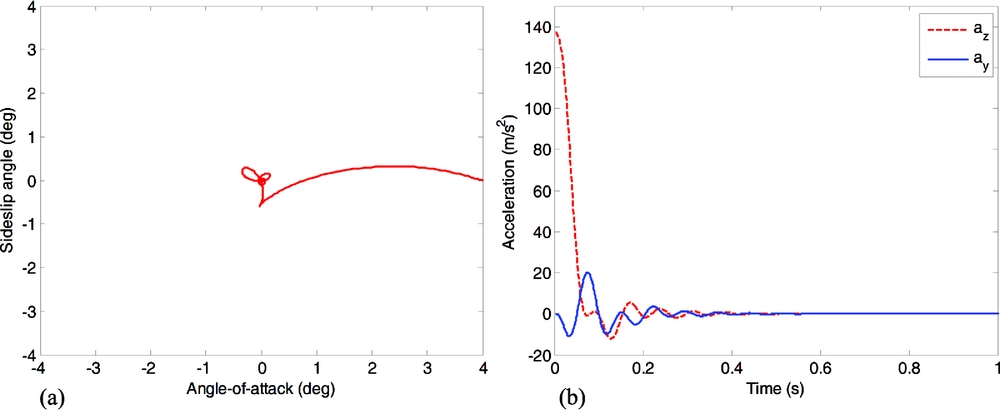
Figure 3. Stable coning motion with kp = 0.5.
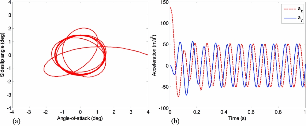
Figure 4. Critical state of coning motion with kp = 0.803.

Figure 5. Unstable coning motion with kp = 0.82.
To further investigate the influence of design parameters on stable regions, the maximum values of kp for stability under different conditions are summarised in Table 2, where the default values of the parameters, not specified in Table 2, are the same as those used in simulations for Figs. 2-5. It follows from Table 2 that the higher the spinning rate is, the smaller the upper limit of kp becomes. For a high spinning rate, Table 2 also shows that one can increase the value of k ω or kz to obtain a larger stable region. Moreover, the larger the scaling factor error or navigation ratio is, the narrower the stable region is. Interestingly, in the presence of large scaling factor error or navigation ratio (see the last line in Table 2), the spinning rate plays a minor influence on the stable regions. This phenomenon also reveals that the parasitic loop induced by scaling factor error severely narrows the stable region and there exists a trade-off design for the navigation ratio between guidance precision and coning motion stability.
Table 2 Maximum values of kp for stability under different conditions

5.0 CONCLUSIONS
A sufficient and necessary condition of coning motion stability for spinning missiles with strapdown seekers is derived analytically and verified using numerical simulations. The results reveal that the parasitic loop induced by scaling factor error, navigation ratio and spinning rate play important roles in the stable region and, therefore, the autopilot gains must be carefully checked using the proposed criteria during the design process to satisfy the stability condition. Future work will consider real-time identification of scaling factor error and dynamic decoupling method to increase the stable region under certain conditions.
ACKNOWLEDGEMENTS
This work was supported by the National Natural Science Foundation of China (Grant No. 61172182).
APPENDIX A. STABILITY CRITERIA OF COMPLEX COEFFICIENT SYSTEM
This section collects a useful lemma regarding the stability of a complex coefficient system, which plays a key role in stability analysis of the closed-loop guidance system.
Lemma 1. (Reference Li, Yang and Zhao16,Reference Li, Yang and Zhao17) Consider the following complex coefficient polynomial
 $$\begin{equation}
{\lambda ^3} + \left( {{p_1} + i{q_1}} \right){\lambda ^2} + \left( {{p_2} + i{q_2}} \right)\lambda + \left( {{p_3} + i{q_3}} \right) = 0
\end{equation}$$
$$\begin{equation}
{\lambda ^3} + \left( {{p_1} + i{q_1}} \right){\lambda ^2} + \left( {{p_2} + i{q_2}} \right)\lambda + \left( {{p_3} + i{q_3}} \right) = 0
\end{equation}$$
The sufficient and necessary condition for all the roots of Equation (A.1) in the left-half of the complex plane is that the three inequalities c 0 > 0, c 1 > 0 and c 2 > 0 are satisfied simultaneously, where
 $$\begin{equation}
\begin{array}{@{}l@{}} {c_0} &=& {p_1}\\
{c_1} &=& \left( {p_1^2{p_2} - {p_1}{p_3} + {p_1}{q_1}{q_2} - q_2^2} \right)/c_0^3\\
{c_2} &=& \left[ {\left( {p_1^2{p_2} - {p_1}{p_3} + {p_1}{q_1}{q_2} - q_2^2} \right)\left( {{p_1}{p_2}{p_3} - p_3^2 + {p_1}{q_2}{q_3}} \right)} \right.\\
&& { -\, {{\left( {p_1^2{q_3} - {p_1}{p_3}{q_1} + {p_3}{q_2}} \right)}^2}} \big]/\left( {c_0^6c_1^3} \right) \end{array}
\end{equation}$$
$$\begin{equation}
\begin{array}{@{}l@{}} {c_0} &=& {p_1}\\
{c_1} &=& \left( {p_1^2{p_2} - {p_1}{p_3} + {p_1}{q_1}{q_2} - q_2^2} \right)/c_0^3\\
{c_2} &=& \left[ {\left( {p_1^2{p_2} - {p_1}{p_3} + {p_1}{q_1}{q_2} - q_2^2} \right)\left( {{p_1}{p_2}{p_3} - p_3^2 + {p_1}{q_2}{q_3}} \right)} \right.\\
&& { -\, {{\left( {p_1^2{q_3} - {p_1}{p_3}{q_1} + {p_3}{q_2}} \right)}^2}} \big]/\left( {c_0^6c_1^3} \right) \end{array}
\end{equation}$$
Proof. Readers can refer to(Reference Li, Yang and Zhao16,Reference Li, Yang and Zhao17) for details.


