1. INTRODUCTION
Geostationary Earth Orbit (GEO) satellites have been widely utilised in the field of communication, meteorology, reconnaissance, navigation, time service, tracking and data relay and scientific research, owing to the high-altitude stationarity relative to the ground and wide signal coverage (Du et al., Reference Du, Li and Wang2012; Vishwakarma et al., Reference Vishwakarma, Chauhan and Aasma2015; Cao et al., Reference Cao, Yang, Su, Li, Chen, Li, Sun, Yao, Wei and Feng2014; Reference Cao, Yang, Li, Chen and Feng2016). Since equatorial space resources are limited, two or more satellites are normally collocated in the same dead box, which requires strict orbit control to avoid potential satellite collisions (Kawase, Reference Kawase2012). However, the orbit determination for GEOs, especially for non-cooperative satellites, remains difficult, because of: (1) the poor observation geometry due to the high orbital altitude, (2) the weak dynamic constraints for ground-based observations owing to the geostationary characteristics, and (3) the frequent orbit manoeuvring conducted to maintain their assigned positions (Du et al., Reference Du, Li and Wang2012, Huang et al., Reference Huang, Hu, Zhang, Jiang, Guo, Wang and Shi2011).
Radio interferometry has advantages of very high angular resolution and insensitivity to weather changes (Tan and Chen, Reference Tan and Chen2015). For example, Very Long Baseline Interferometry (VLBI), with less than 0·001” of angular tracking accuracy, has been widely used to determine positions of extragalactic radio sources for several decades in the field of astronomy. Further, it has been an important development for the realisation and maintenance of the International Celestial Reference Frame (ICRF) (Schuh and Böhm, Reference Schuh and Böhm2013). VLBI is also used to track spacecraft during deep space exploration (Tan and Chen, Reference Tan and Chen2015).
As for GEOs, VLBI is expected to provide a Three-Dimensional (3D) position accuracy of 3 m (Ellis, Reference Ellis1984; Shiomi and Kawano, Reference Shiomi and Kawano1987). Huang et al. (Reference Huang, Hu, Zhang, Jiang, Guo, Wang and Shi2011) used VLBI data from the Chinese VLBI Network (CVN), in combination with C-band range data, to determine a GEO satellite's orbit to an accuracy of about 10 m. Despite its effectiveness, the VLBI technique is unlikely to be adopted for routine orbit determination of GEOs because it is expensive and inefficient, and requires large aperture antennae, highly precise atomic frequency standards, low-thermal noise and high-speed data acquisition and processing.
Connected-Element Interferometry (CEI), a type of smaller-scale radio interferometer, is applicable to common clocks, to distribute time and frequency signals through a fibre-optic link or coaxial cable to nearby antennae, which ensures coherent operation and no need to solve for the clock rate offset between stations (Edwards et al., Reference Edwards, Rogstad, Fort, White and Iijima1992). The National Aeronautical and Space Agency (NASA) first applied CEI to the navigation of deep space spacecraft owing to the simplicity of the measurement system, low construction cost and near-real-time correlation of the incoming signals (Thurman and Badilla, Reference Thurman and Badilla1990; Edwards et al., Reference Edwards, Rogstad, Fort, White and Iijima1992; Wu et al., Reference Wu, Huang, Hong, Jie and Li2015). The main factors affecting CEI measurement accuracy are the baseline length, frequency reference, signal transmission conditions and calibration system, and some research has been conducted as follows.
Normally, the baseline length of CEI trials is less than 200 km. McCarthy et al. (Reference McCarthy, Kaplan, Klepczynski, Josties, Matsakis, Angerhofer, Johnston and Spencer1980) utilised CEI and optical instruments to determine Earth rotation parameters with a 35 km baseline. Morrison et al. (Reference Morrison, Pogorelc, Celano and Gifford2002) used a 180 km baseline to track Global Positioning System (GPS) and GEO satellites to determine orbit accuracies of 30 metres and 3 km for GPS and GEO satellites, respectively. Li et al. (Reference Li, Huang and Pan2010) analysed the influences of varying length, location and orientation of the baseline, as well as the observation arc, on the orbit determination accuracy of GEOs with simulated data. Ren et al. (Reference Ren, Tang, Cao, Chen, Han, Wang and Li2016) carried out a 5·5 km single baseline test for a GEO satellite, indicating that the solution can converge with a long observation arc, while the orbital accuracy was only 35·7 km. Kawase and Sawada (Reference Kawase and Sawada1999) used a Same-Beam CEI (SBI) to track two GEOs with a 130 metre baseline, and the results suggested that SBI is capable of measuring the relative position of the GEOs at the level of a few hundred metres.
CEI shares time and frequency signals coming from one common clock to all the antennae, owing to its small-scale. A high-quality commercial rubidium clock is sufficiently precise as a frequency reference for CEI (Huang et al., Reference Huang, Li and Hao2014). Wang et al. (Reference Wang, Wang, Li and Yang2014) proposed an improved interferometry signal processing algorithm for when the Signal to Noise Ratio (SNR) is low, which is capable of increasing the measurement accuracy.
To improve the precision and stability of phase measurement, the calibration system was augmented to cancel the influence of ambient temperature variations on signal transmission by Kawase (Reference Kawase2012). The test results showed that, usually, the longer the transmission cable, the noisier the observation data. However, phase fluctuations can be stabilised within 1° by adding calibration.
Among the previously stated issues, a baseline length of several kilometres or longer can improve angular resolution but is not suitable for space-limited tracking stations. The monitoring of the relative orbital motions has high precision but can only be used for closely operating geosynchronous satellites. The influences of sunlight and the calibration signal on phase fluctuation have been investigated, but there is no analysis of the influence on orbit determination accuracy. These factors limit the widespread application of CEI.
In this work, we focus on the application of CEI with orthogonal double baselines (75 m × 35 m) for GEO satellite orbit determination. This paper begins with a short description of the characteristics of the CEI technique, measurement principles and model. Second, the CEI system is introduced and applied to monitor a GEO TV satellite. Phase data and a method of integer ambiguity determination are investigated. Finally, a precise orbit of the GEO satellite is obtained by using a batch algorithm and the orbit accuracy, as well as main error sources for orbit accuracy, are analysed.
2. CEI PHASE OBSERVATION
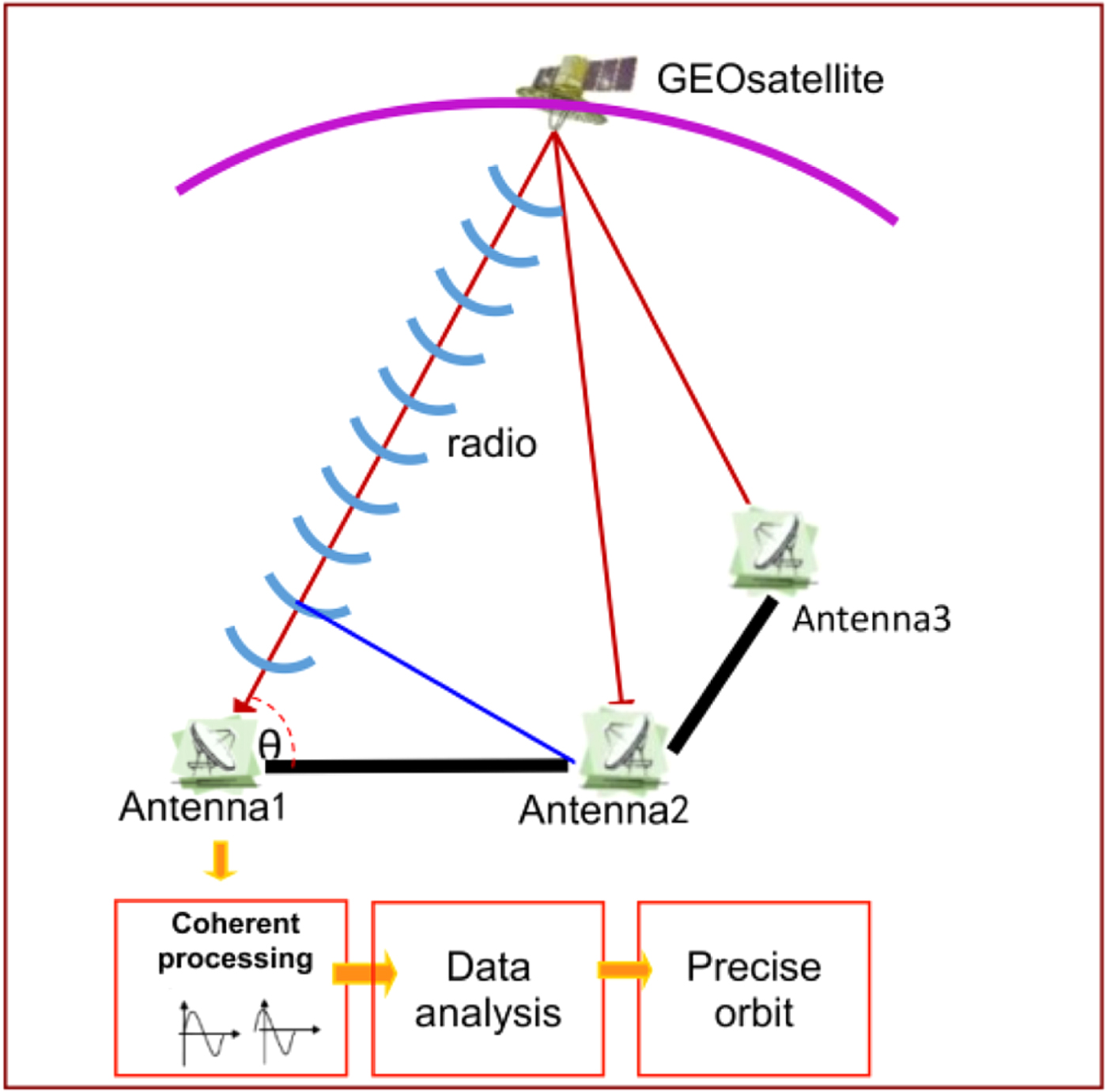
To obtain angular information in a certain direction, a real-time CEI measurement system needs at least two stations. Therefore, a complete CEI measurement system requires at least three stations, which form two baselines perpendicular to each other. Each station consists of a receiving antenna, Low Noise Block (LNB), and frequency mixer, and the data processing centre consists of down converter, and a data receiving, processing and recording system. The measurement principles of CEI are shown in Figure 1.

Figure 1. Schematic diagram of CEI operating principle.
For a baseline length of less than 100 km, the basic and prominent observation of CEI is the phase delay rather than the group delay. The phase observation equation can be established according to the signal propagation of a spherical wave, namely:
 $$\eqalign{\phi +\lambda N & =\rho_A -\rho_B \cr & =\vert {\mathop{R} \limits^{\rightharpoonup}}_{A} \lpar t_1\rpar -{\mathop{r} \limits^{\rightharpoonup}}\lpar t_0 \rpar \vert -\vert {\mathop{R} \limits^{\rightharpoonup}}_B \lpar t_2\rpar - {\mathop{r} \limits^{\rightharpoonup}} \lpar t_0 \rpar \vert +c\Delta t_{clock} +\Delta \rho _{atm} +\Delta \rho_{ins} +\varepsilon} $$
where ϕ and N are the measurement phase and the integer ambiguity, respectively; λ is the signal wavelength;  ${\mathop{R} \limits^{\rightharpoonup}}_{A}$ and
  ${\mathop{R} \limits^{\rightharpoonup}}_{B}$ are the position vectors of the satellite and baseline stations A and B, respectively; Δt clock is the clock difference between the two stations; Δρ atm is the residual error of atmospheric propagation delays through the troposphere and ionosphere between the satellite and the two stations; Δρ ins is the difference in equipment delays and ε is the noise. Note that the accurate phase data is not usable for precise orbit determination until this integer ambiguity has been properly resolved. In this paper, we use Two-Line Element (TLE) data as the a priori orbit information to determine integer ambiguity.
3. CEI SYSTEM ARCHITECTURE
The CEI experimental system consists of three parts: outdoor equipment, indoor equipment and calibration subsystem. The outdoor equipment mainly consists of a receiving antenna and LNB; the indoor equipment consists of data receiving, processing and storing, as well as the corresponding hardware and software. The calibration system consists of a signal generator and a frequency divider, as shown in Figure 2.
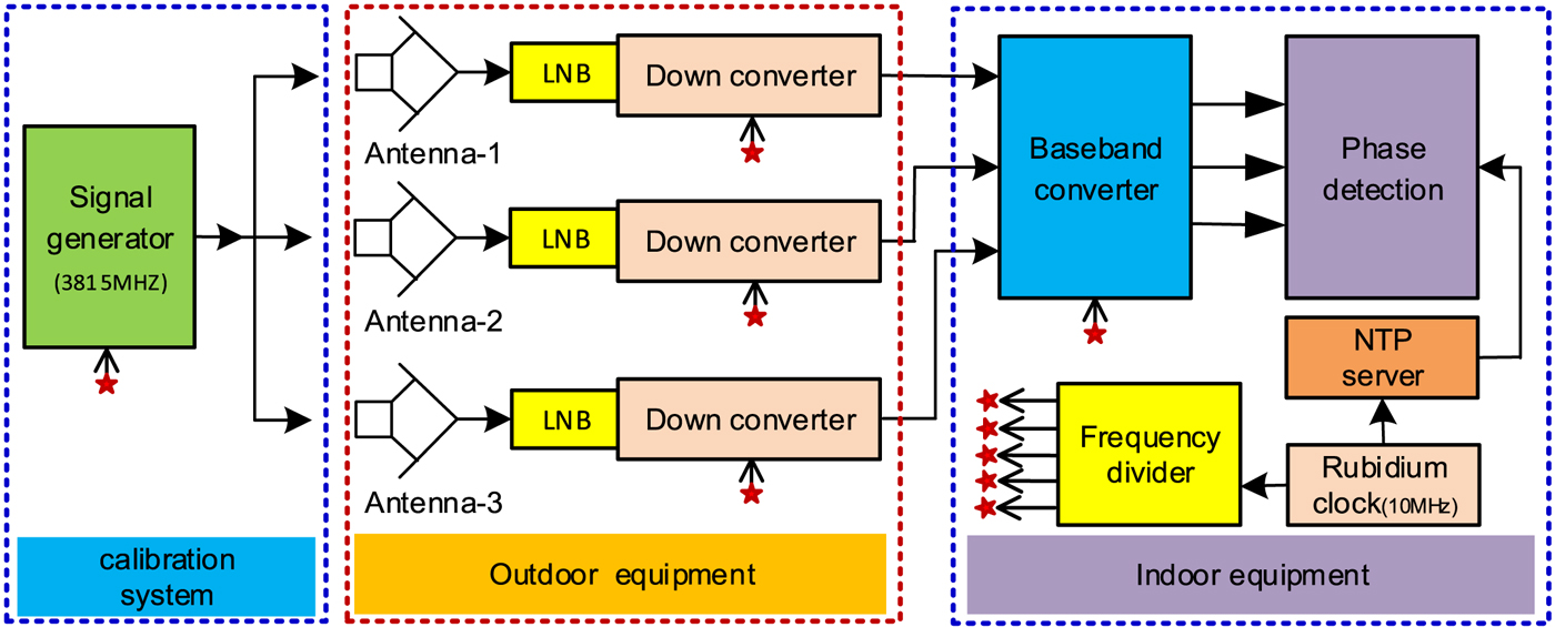
Figure 2. Block diagram of CEI experimental system.
3.1. Outdoor equipment
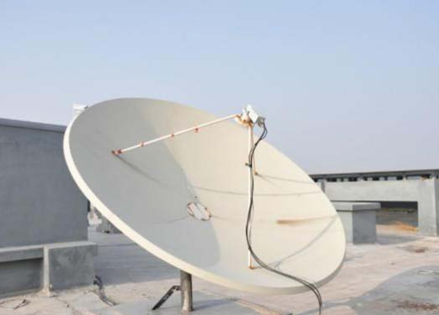
The outdoor equipment consists of three 2.4 m antennae (east-west distance 75 m, north-south distance 35 m), and LNB (with first order frequency conversion capability). Every antenna is connected by 100 m coaxial cable (including a low-noise amplifier power cable, a local oscillator uplink cable, and an intermediate frequency down cable) to the indoor signal processing equipment, as shown in Figure 3.

Figure 3. C band receiving antenna.
3.2. Indoor equipment
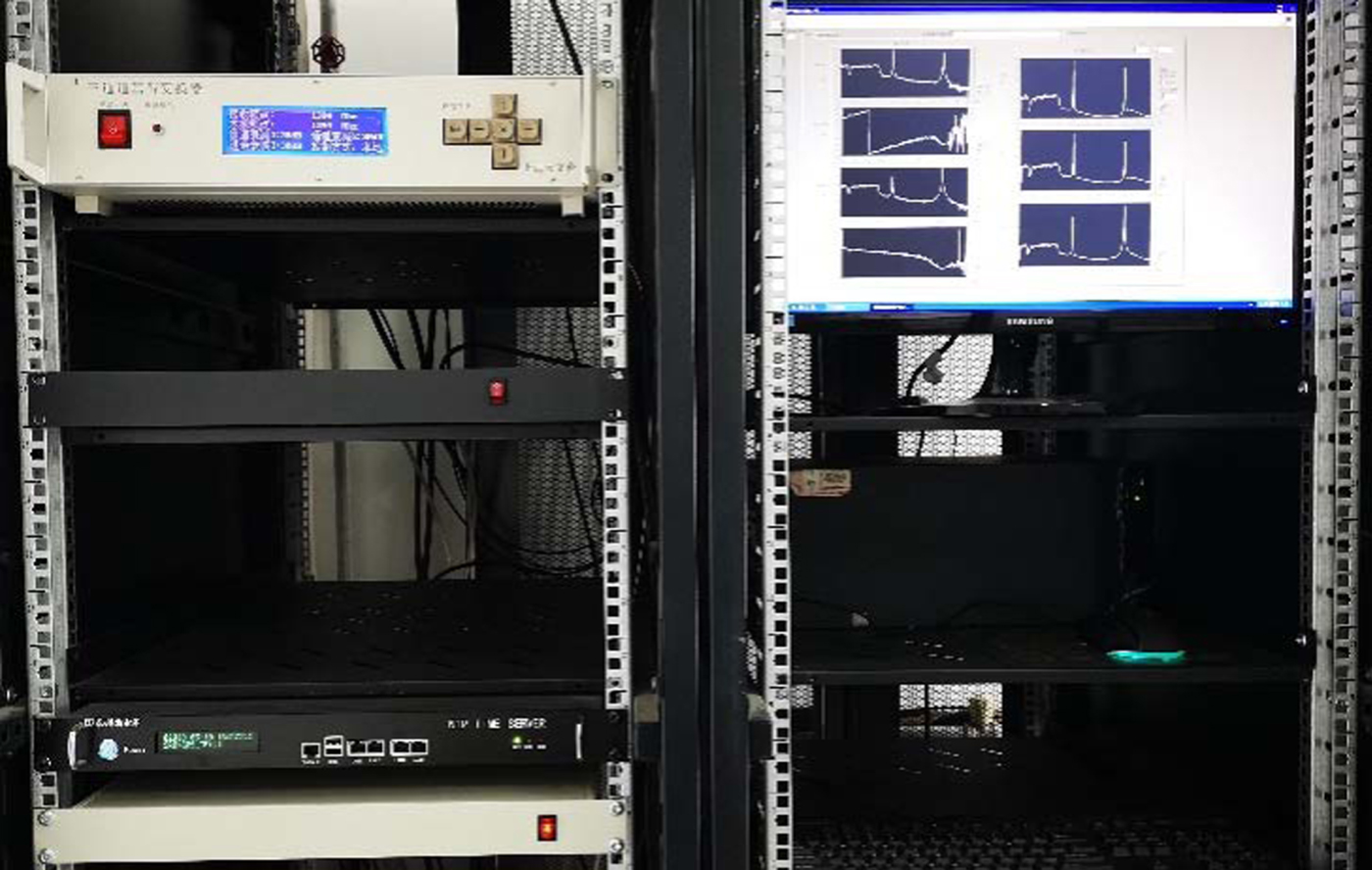
The indoor equipment consists of a power supply, a signal distributor, a baseband frequency converter, a rubidium atomic clock, and a computer (a data acquisition card and data visualisation and storage software), as shown in Figure 4. The accurate phase measurement of a GEO satellite can be extracted from the correlation results; then, the precise orbit of the satellite can be obtained using a batch algorithm.

Figure 4. Indoor equipment.
3.3. Calibration system
The calibration system is designed mainly to eliminate the complex disturbances of the cabled signal downlink transmission. It consists of calibration signal generation, transmission and reception. The calibration signal is generated indoors, transmitted to up to three antennae, synchronously received by the antennae together with the satellite signal, and then transmitted back to the indoor equipment for subsequent correlation processing.
The final observations are the calibrated phases with the phase delay of the calibration signal subtracted from the original observation. To obtain optimal calibration, the nearest frequency to that of the satellite signal is adopted for the calibration system, given that the two signals are discriminable.
4. RESULTS AND DISCUSSIONS
4.1. Experiment setup
The observation conditions were as follows:
(1) The GEO satellite: ChinaSat 10, the assigned longitude was 110·5°E, with 30 C-band and 16 Ku-band transponders;
(2) The antennae were located at Zhengzhou (34·4°N, 113°E);
(3) CEI data set: three days of observation, starting from 01:00 (UTC), 5 December 2016;
(4) The tracking frequency of the GEO: 3,817 MHz;
(5) The frequency of the calibration signal: 3,815 MHz.
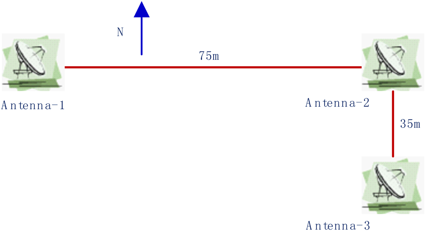
The layout of the outdoor antennae is shown in Figure 5. The east-west baseline, with a length of 75 m, consists of antenna 1 and antenna 2, while the north-south baseline, with a length of 35 m, consists of antenna 2 and antenna 3.

Figure 5. Antennae and CEI baselines (75 m × 35 m).
The sampling rate of the acquisition card was 10 MHz, the number of Fast Fourier Transform (FFT) points was 1,024, and the integral time was 1 s, that is, 512 complex numbers could be obtained per second. The output data consisted of a real part, imaginary part, amplitude and phase angle of the cross-correlation spectra for the antenna 1–2 baseline and the antenna 2–3 baseline.
4.2. Analysis of 30 min observations
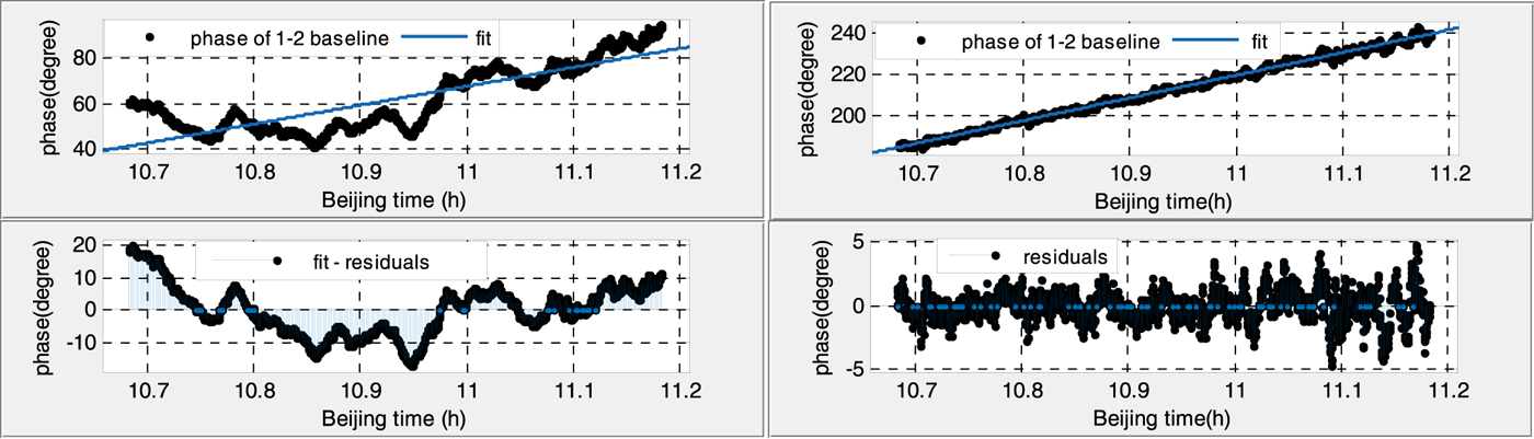
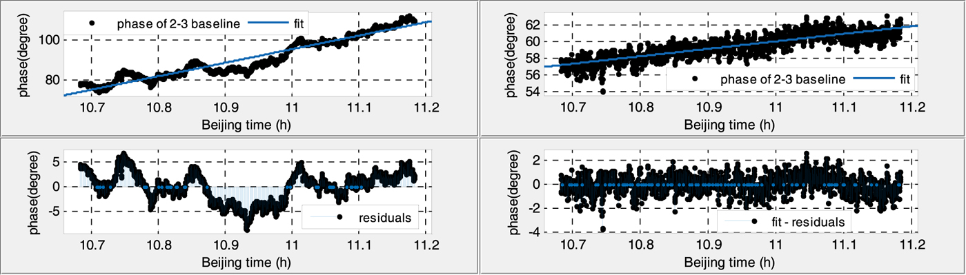
Figures 6–9 show the 30 min phases of two baselines in daytime and at night, before (left) and after (right) calibration.

Figure 6. Phase variation of the antenna 1–2 baseline in the daytime (before calibration Root Mean Square (RMS): 7·787 (left), after calibration RMS: 1·218 (right)).
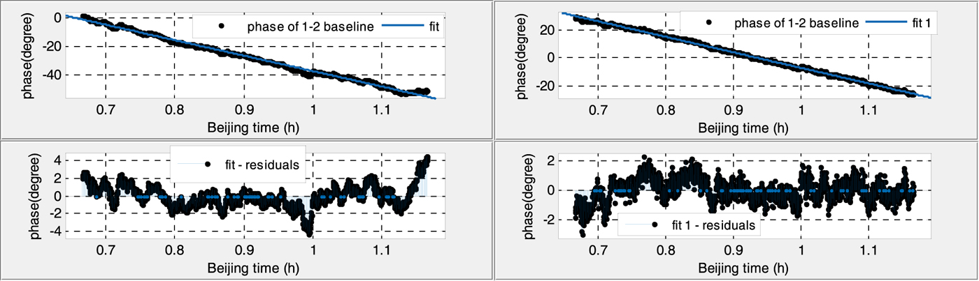
Figure 7. Phase variation of the antenna 1–2 baseline at night (before calibration RMS: 1·277 (left), after calibration RMS: 0·7745 (right)).

Figure 8. Phase variation of the antenna 2–3 baseline in the daytime (before calibration RMS: 2·892 (left), after calibration RMS: 0·744 (right)).
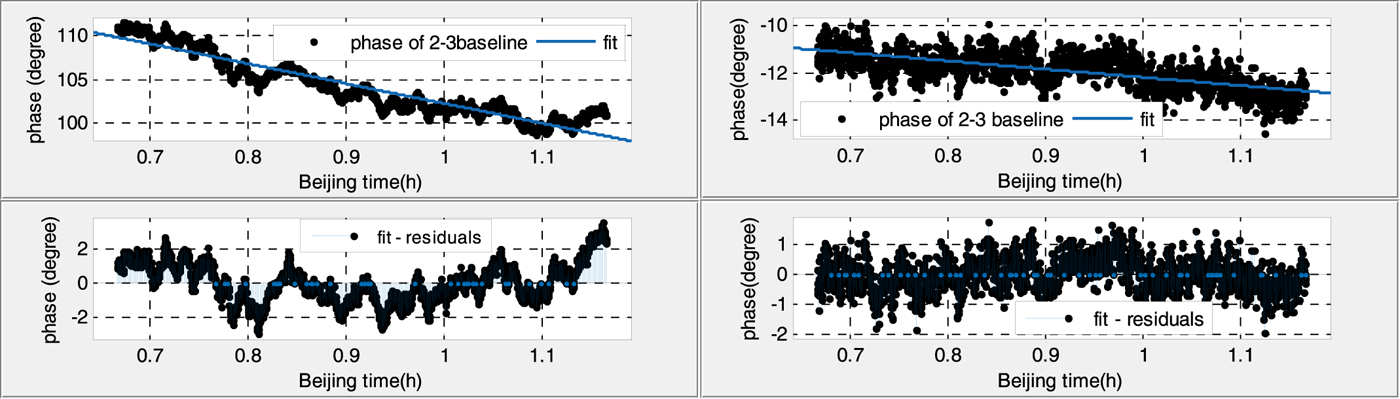
Figure 9. Phase variation of the antenna 2–3 baseline at night (before calibration RMS: 1·150 (left), after calibration RMS: 0·5472 (right)).
(1) Without calibration, the phase residuals of linear fitting in the daytime are six times larger and twice as large than that at night for both baselines, which suggests that the phase variations are strongly affected by temperature.
(2) With the calibration signal, the fitted phase residuals decrease significantly, and phase variations during the whole day tend to be a stable value, less than 1·5°, which also indicates the necessity of the calibration.
4.3. Long-time phase variations of satellite signal and calibration signal
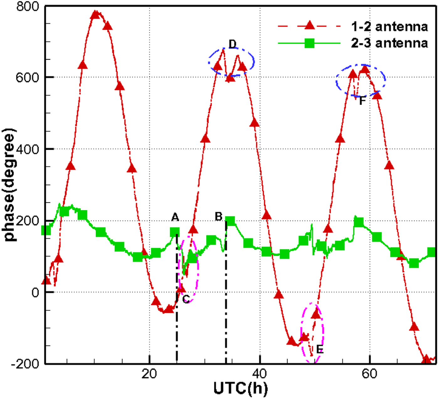
Even without calibration, the phases of the antenna 1–2 baseline present distinct diurnal variations, consistent with the orbital period of the GEO satellite (see Figure 10). However, the length of the 2–3 baseline is only 35 m, nearly half of that of the antenna 1–2 baseline. The phases on the shorter baseline have a limited variation scale of 150°, and it is more difficult to observe the diurnal trend when disturbed by the phase jumps.

Figure 10. Phase variation of satellite signal.
Moreover, it can be observed that certain phase jumps occur almost simultaneously for both baselines. For example, point A and B for the antenna 2–3 baseline and point C and D for the antenna 1–2 baseline. These jumps occur at around 09:00 and 17:00, Beijing time, which corresponds to sunrise and sunset (the three days were sunny). The reason for this is that some parts of the cables were outdoors and were not covered with insulation materials in this test; the phases were directly affected by the changes in cable temperature.
Figure 11 illustrates the phases of the calibration signal during the same time interval. Phase jumps also occur, which indicates that the changes of cable temperature also affect the phases of the calibration signal.
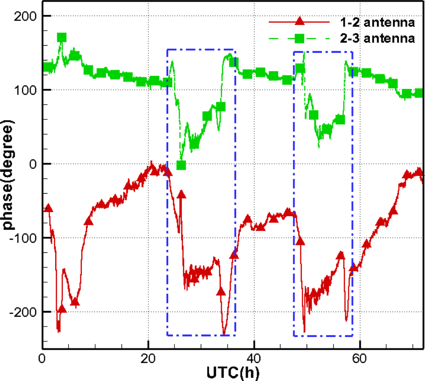
Figure 11. Phase variation of calibration signal.
Fortunately, the epochs and duration of those phase jumps are consistent for the two kinds of signals (see circle D and F in Figure 10, and the two blue dotted rectangles in Figure 11). Therefore, the calibration signal has the potential to eliminate most phase jumps and improve the quality of the observations.
It should be noted that the calibration signal has effects on the disturbances of transmission cables and instruments, but no effects on the disturbances of the satellite signal space transmission.
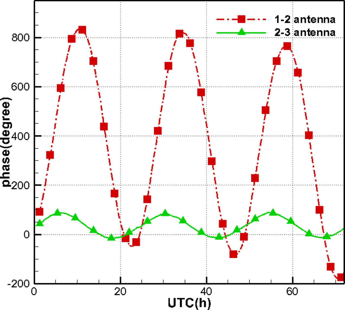
Figure 12 illustrates the calibrated phases of the satellite signals. Compared with Figure 10, most phase jumps have been eliminated, particularly for data in the daytime, and the diurnal variations for the antenna 2–3 baseline can be seen clearly. Therefore, the dataset hereinafter merely uses the calibrated phases.

Figure 12. Phase variation of satellite signal after calibration.
4.4. Phase ambiguity solution
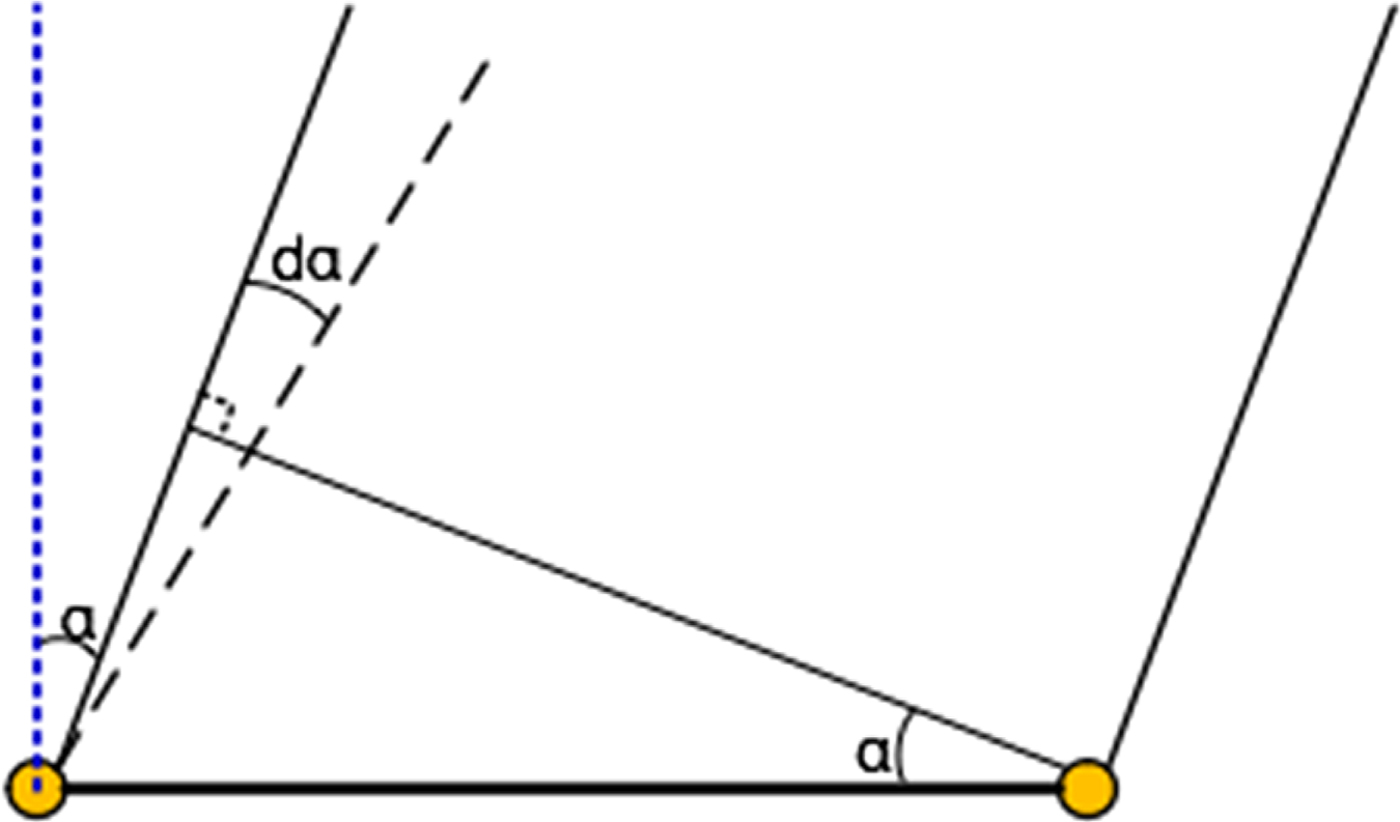
The resolved phase ambiguity is a prerequisite for using phase data. Figure 13 is a diagram of the GEO satellite and a baseline. The angle α is the complementary angle of the direction of the satellite relative to the baseline, and the observation phase can be simply expressed as:

Figure 13. Problem of phase ambiguity.
 $$\phi =\displaystyle{{2\pi }\over{\lambda }}B\sin \alpha $$
Differentiating Equation (2), we have:
 $$d\phi =\displaystyle{{2\pi }\over{\lambda }}B\cos \alpha d\alpha $$
In this test, the length of the baseline is accurate, and the observation band of the downlink signals is selected. The angle α is 5·5° and 30·5° for the antenna 1–2 and antenna 2–3 baselines, respectively. Therefore, we have d ϕ = 6254 · 3d α for the antenna 1–2 baseline and d ϕ = 2526 · 4d α for the antenna 2–3 baseline.
As long as the prior orbit of the satellite is accurate enough and the calculated d ϕ with the angular error d α is less than 2π, the integer ambiguity can be resolved.
Herein, we use TLE, with an accuracy of 10–20 km, to calculate the prior orbit of the satellite.
4.4.1. Determination of integer ambiguity
The ambiguity is resolved with a single epoch. From Equation (1), the phase ambiguity (N) can be determined using the a priori satellite position predicted by TLE. As the baseline lengths are short, and the length of the transmission cables (Intermediate Frequency (IF) downlink cables and clock signal cables) is roughly equal (100 m), most residual errors (including the propagation error of the troposphere and ionosphere) in the transmission path of Radio Frequency (RF) signals are cancelled out, and we do not need to modify the delay in the RF signal transmission path and clock errors:
 $$\Delta t_{clock} \approx 0 \quad \Delta \rho _{atm} \approx 0 $$
Then, the phase ambiguity (N) can be simplified as:
 $$N=\hbox{int}\left[{\displaystyle{{\rho_A -\rho_B }\over{\lambda}}} \right]$$
By comparing the calculated phase (ϕ C ) with the observation phase, the instrument delay (Δρ ins) can be written approximately:
 $$\Delta \rho _{ins} =\phi -\phi _C $$
4.4.2. Ambiguity resolved phase delay
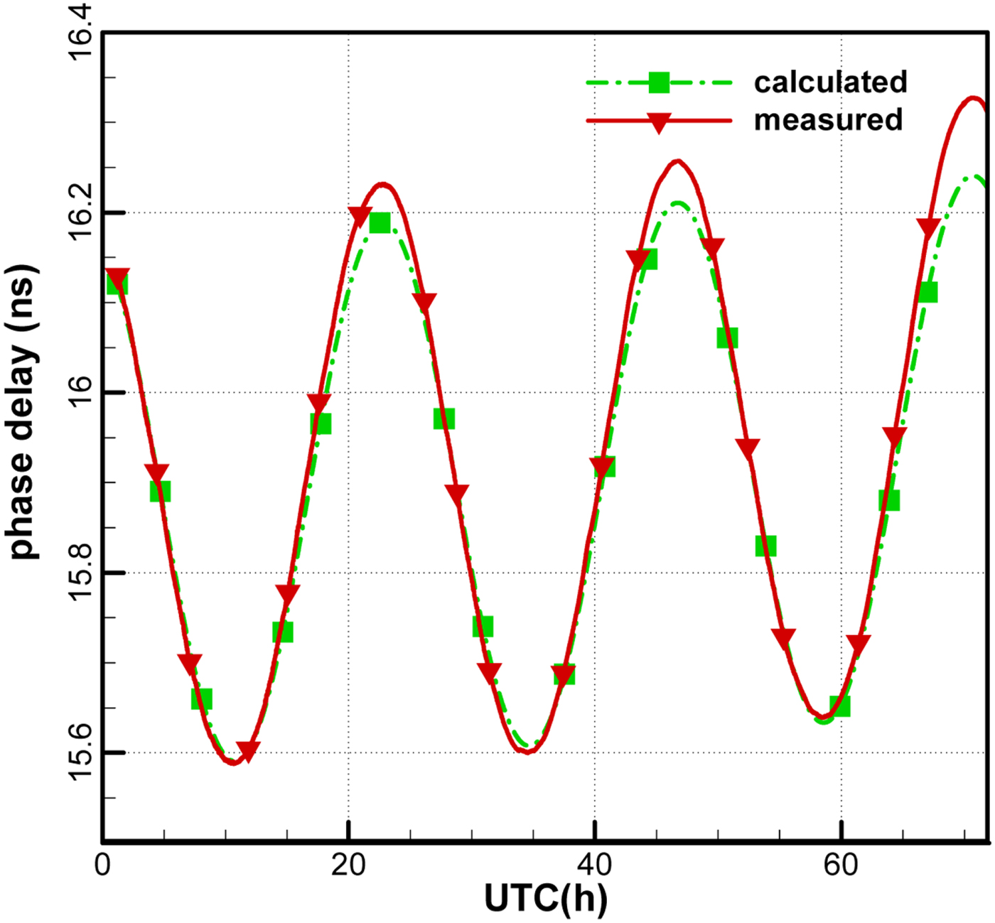
Figures 14 and 15 show the observation phase delays and the calculated phase delays (in ns) of the two baselines. It can be seen that the variations of the two phase delays are consistent, which suggests that the publicly downloaded TLE can provide an accurate predicted orbit to solve ambiguity. However, the departures increase gradually with the prediction time due to the accumulated orbital error. Therefore, it would be better to adopt the nearest updated TLE of the satellite.

Figure 14. Ambiguity resolved phase delay for the antenna 1–2 baseline.
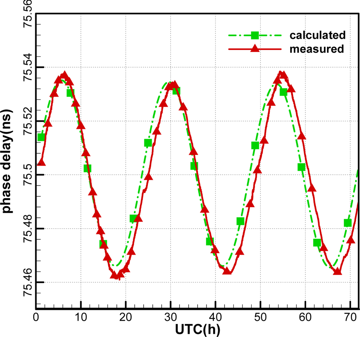
Figure 15. Ambiguity resolved phase delay for the antenna 2–3 baseline.
Figure 16 shows the residuals of the observation phase delay minus the calculated phase delay. Even with the calibration system, diurnal variations still exist in the residuals and are slightly smaller at night than in the daytime. The variation scale of the antenna 2–3 baseline is at the level of 0.02 ns, while that of the antenna 1–2 baseline can reach 0.05 ns within the first 48 h. It should be mentioned that station 1 is the furthest, and most cables to this station were exposed to sunlight, which also reduces the effects of temperature for the 1–2 baseline. Therefore, it is expected that the delay residuals of the 1–2 baseline can reach the same level as that of the 2–3 baseline by covering the insulation materials for the cable of station 1.
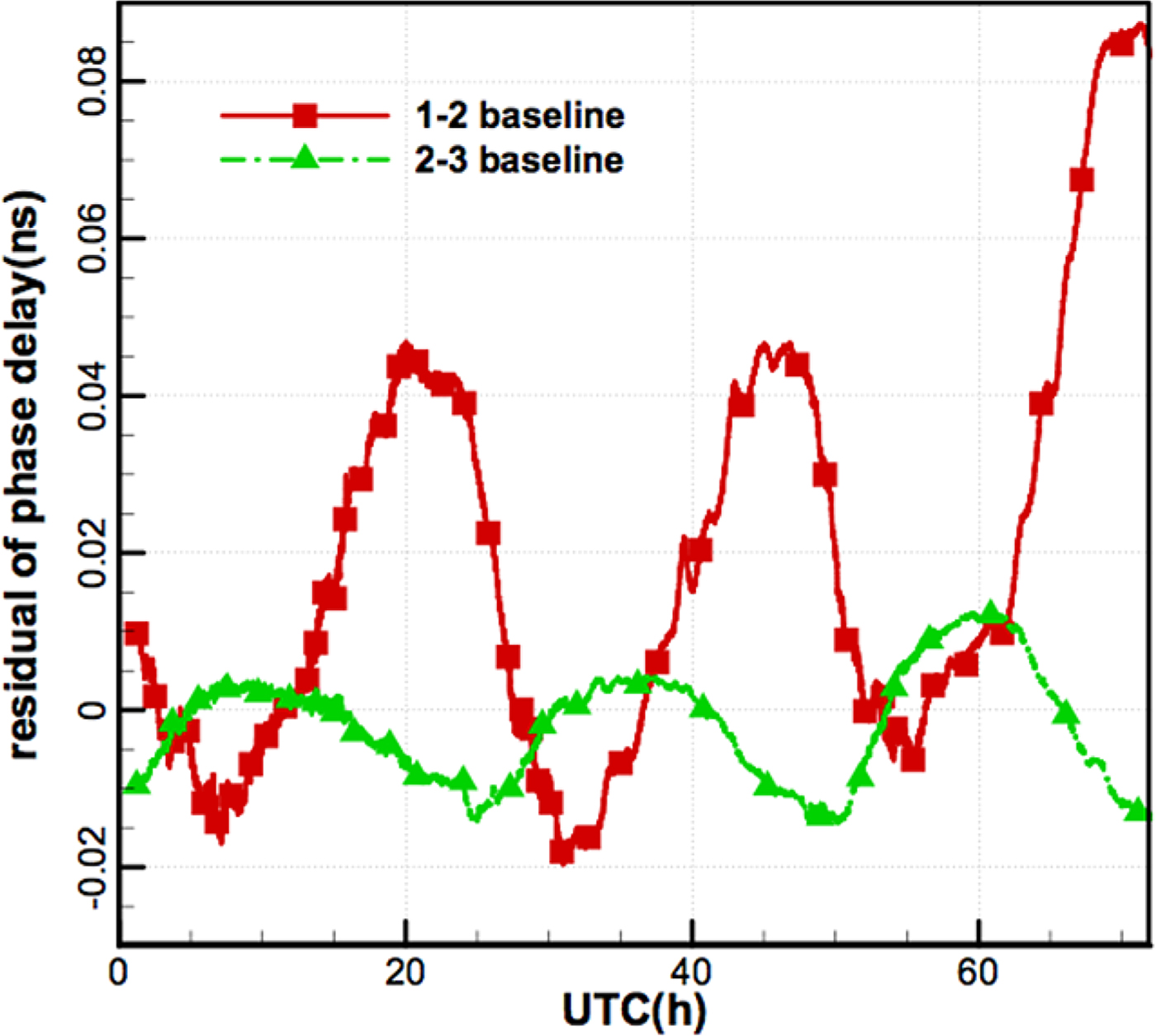
Figure 16. Residuals of phase delay of the two baselines.
4.5. Results of orbit determination
4.5.1. Orbit determination strategy
Batch algorithms were used to estimate six orbital elements of the GEO satellite. Different orbit arcs (6 h–66 h) were considered, starting from 01:13:00, 5 December 2016 (UTC), with a 60 s sample rate. The satellite dynamics were modelled by numerically integrating the equations of motion, which included the following dynamic effects:
• Geopotential model: GGM03C gravity field for up to degree and order ten.
• Third-body gravitational effects: gravitational tidal potentials of the Sun and Moon.
• Solar radiation pressure: spherical model for GEO.
Solar and Lunar ephemerides were computed using the DE405 planetary ephemeris, and Earth orientation parameters were derived from the latest data published by the International Earth Rotation and Reference Systems Service (IERS). To assess the CEI-based orbit accuracy, we used orbits provided by the China National Time Service Center (NTSC) as Precise Ephemeris (PE), which indicates a 10 m orbit accuracy in comparison with the Satellite Laser Ranging (SLR) results.
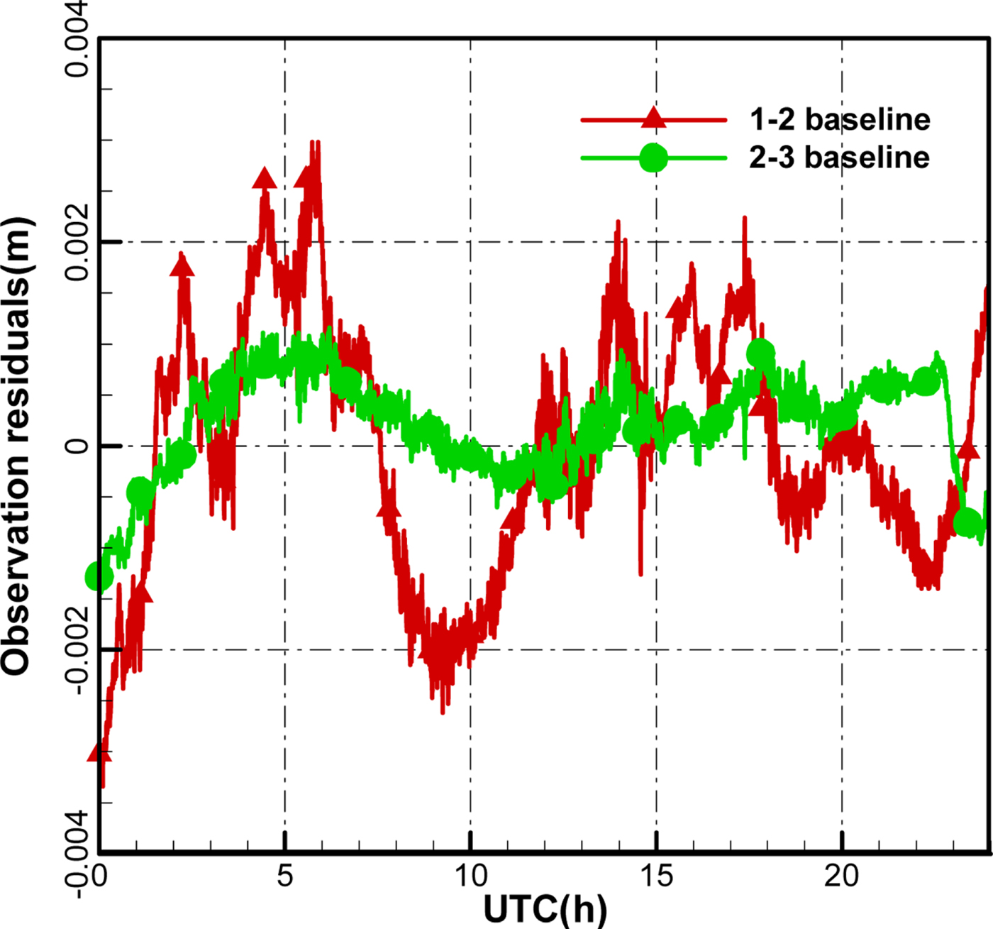
4.5.2. The observation residual
Figure 17 is the time series of the Precise Orbit Determination (POD) residuals of CEI data for about 24 h. The RMS of the antenna 1–2 baseline and the antenna 2–3 baseline data are about 1.195 mm and 0.523 mm, respectively. Figure 17 shows different noise levels for the antenna 1–2 baseline and the antenna 2–3 baseline, and the accuracy for the antenna 2–3 baseline is lower than that of the antenna 1–2 baseline, which may be due to more remarkable changes of the cable temperature for the antenna 1–2 baseline. The sun can shine directly on most of downlink cables of antenna 1, which intensifies inconsistencies with the two-antenna downlink cable environment.

Figure 17. The observation residual after orbit determination for 24 h.
4.5.3 Orbit determination accuracy
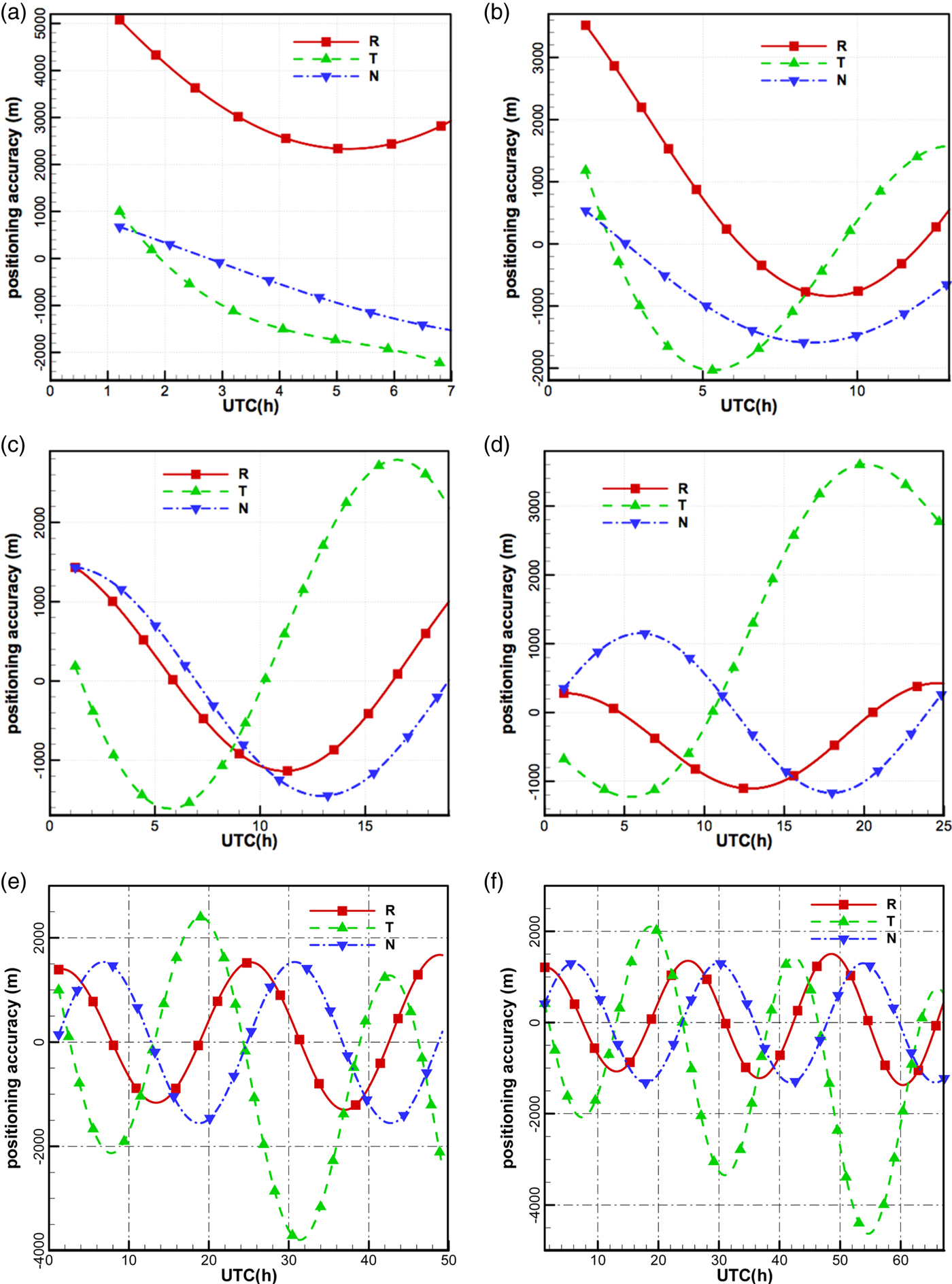
Figures 18(a–f) show the orbital differences between POD using CEI data and the precise ephemeris over different observation arcs. With the increase of observation arc, the trends (diurnal variations) of accuracy gradually appear, owing to diurnal variations of observation quality. Comparing with Figure 16, the variations of the accuracy in the along-track direction are consistent with the phase delay residuals of the antenna 1–2 baseline, and the variations of the accuracy in the cross-track direction are consistent with the phase delay residuals of the antenna 2–3 baseline.

Figure 18. Orbital differences between POD using CEI data and the precise ephemeris.
The accuracies in the radial direction and in the cross-track direction are improved with the increase in observation arc, particularly in the radial direction, since dynamic constraints are gradually strengthened. The accuracy in the along-track direction is lower than in the other two directions when the observation arcs are more than 18 h.
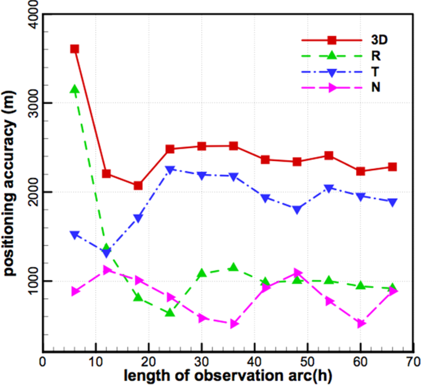
Table 1 and Figure 19 show the RMSs of differences between POD using CEI data and the precise ephemeris over different observation arcs, respectively, and conclusions can be drawn as follows:
(1) With the increasing observation arc, the 3D position accuracy can reach an order of 2 km. Since the orbit period is about 24 h, at least a 24 h observation arc is required for this measurement system. Comparing the results with existing works of Ren et al. (Reference Ren, Tang, Cao, Chen, Han, Wang and Li2016), the orbit determination accuracy is improved by an order of magnitude.
(2) Increasing the observation arcs can effectively improve the orbit determination accuracies in the radial direction, when observation arcs are less than 24 h, because CEI data have no constraints in this direction, and the improvements of accuracy mainly depend on dynamic constraints. Since the orbit period is about 24 h, the RMS of orbit difference reaches a minimum (636·28 m) for the 24 h observation arc.
(3) Both CEI data constraints and dynamic constraints affect the accuracy in the along-track direction and in the cross-track direction. When observation arcs are short (such as 6 h and 12 h), the dynamic constraints are weaker than CEI data constraints, and the accuracies of these directions depend mainly on the observation quality. Inconsistency in the quality of observations (in the daytime and at night) leads to fluctuations of orbit accuracies (see Table 1 and Figure 19). When observation arcs are longer than 24 h, with dynamic constraints gradually strengthened, the accuracies in the along-track direction and in the cross-track direction can reach an order of magnitude of 2 km and 900 m, respectively.
(4) The accuracy in the along-track direction is obviously lower than that in the cross-track direction. In order to improve the accuracy in the along-track direction, we will increase the antenna 1–2 baseline length, and improve the observation quality of the antenna 1–2 baseline and calibration accuracy of systematic errors in future research.
Table 1. RMS of differences between POD and the precise ephemeris


Figure 19. RMS of differences between POD and the precise ephemeris.
5. CONCLUSIONS
In this study, a CEI system with orthogonal double baselines (75 m × 35 m) has been successfully developed and deployed to track a GEO TV satellite for orbit determination. From the discussions above, the following conclusions can be drawn:
(1) According to the 30 min of sampled phase data at night and in the daytime, the linear fitting phase residuals on both baselines indicate that phase variations are strongly affected by temperature.
(2) For the three days of observation data, the jumps are generally near 09:00 and 17:00 Beijing time, which corresponded to sunrise and sunset. The overall trend of the phase of the antenna 1–2 baseline remains unchanged even with the jumps, while the phase of the antenna 2–3 baseline not only presents jumps, but those jumps obviously change the overall tendency. After applying the signal calibrations, the phase jumps are almost eliminated and the quality of observations is remarkably improved, especially in the daytime, which also indicates the necessity of using the calibration signal.
(3) Using TLE as the a priori orbit information to resolve the phase ambiguity is feasible. The orbit determination accuracies show that the orbit determination accuracy is gradually improved with the increase of observation arcs. Meanwhile, the accuracy in the along-track direction is obviously lower than that in the other two directions. When the observation arcs are longer than 24 h, 3D position accuracy reaches the 2 km order of magnitude, the accuracy in the radial direction can reach the 700 m order of magnitude and the accuracy in the cross-track direction can reach the 900 m order of magnitude. Therefore, the measurement system requires at least 24 h observation arcs.
ACKNOWLEDGMENTS
This work was supported by grants 41804034 and 41774038 from the National Natural Science Foundation of China, the opening Project of Shanghai Key Laboratory of Space Navigation and Positioning Techniques fund No. KFKT_201707, and State Key Laboratory of Geo-Information Engineering Laboratory fund No. SKLGIE2016-Z-2-4. The authors also give great acknowledgements and thanks to National Time Service Centre for providing precise ephemeris of the GEO Satellite.