3.1. Isotropic turbulence flow facility

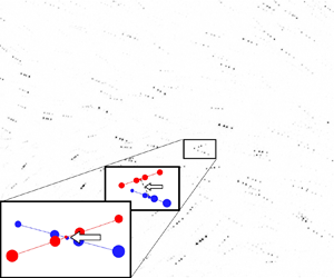
We performed particle tracking in a high Reynolds number enclosed truncated icosahedron homogeneous isotropic turbulence (HIT) chamber (figure 1). This one metre ‘soccer ball’ shaped facility described in Dou et al. (Reference Dou, Pecenak, Cao, Woodward, Liang and Meng2016) is a second-generation isotropic turbulence chamber, improved from the original cubic turbulence box (eight fans with $Re_\lambda$ between 110 and 150) developed for our first attempt of simultaneous RDF and RV measurement (de Jong et al. Reference de Jong, Salazar, Woodward, Collins and Meng2010). The turbulence in the HIT chamber has been completely characterized in the central isotropic region (diameter 4.8 cm) by Dou et al. (Reference Dou, Pecenak, Cao, Woodward, Liang and Meng2016). We held the fan speed constant such that $Re_\lambda =324$ and used 3M K25 hollow glass spheres (3M, St. Paul, Minnesota) as particles, narrowing their diameter range to $25 - 32\ \mathrm {\mu }\textrm {m}$ using sieves, following the procedure in Dou et al. (Reference Dou, Ireland, Bragg, Liang, Collins and Meng2018b). The average density of the sieved particles was measured using a Micromeritics Accu-Pyc II 1340 gas-displacement pycnometer. The resulting particle and flow characteristics are listed in table 1.

Figure 1. The 4P STB system (top view) and timing.

Table 1. Particle and flow conditions. For complete details of turbulence in the HIT chamber see Dou et al. (Reference Dou, Pecenak, Cao, Woodward, Liang and Meng2016).

To reduce complexity of our experiments, we kept the electric charge and gravity effects to a minimum. To minimize triboelectric charging of the particles caused by friction with the fans and walls, the inner surfaces of the turbulence chamber were coated in conductive carbon paint and electrically grounded, as described in Dou et al. (Reference Dou, Ireland, Bragg, Liang, Collins and Meng2018b). This helped to remove the charge on the particles. To mitigate the effect of gravity on the particles, we used fans as flow actuators in our chamber (Dou et al. Reference Dou, Pecenak, Cao, Woodward, Liang and Meng2016), which yielded a high Froude number $Fr=13.4$. Furthermore, due to the low density and large size of our hollow glass spheres, the gravitational settling speed (assuming Stokes drag and a quiescent flow) of our particles was $0.007\ \textrm {m}\ \textrm {s}^{-1}$, compared with the Kolmogorov velocity of $0.13 \ \textrm {m}\ \textrm {s}^{-1}$.

To prevent any transient effects in the statistics of particle motion due to particle injection, the particles were aerosolized, then pneumatically injected into the flow facility and allowed to equilibrate over 100 large eddy turnover times ($\approx$30 s). The particle volume fraction was kept at ${\sim }2.2 \times 10^{-5}$ (equivalent to 0.002 particles per pixel) to remain well within the dilute limit.

3.2. Optical interrogation set-up

3.3. Implementation of STB particle tracking

We implemented our small-$r$ measurement strategy using the multipulse STB tracking algorithm (Novara et al. Reference Novara, Schanz, Geisler, Gesemann, Voss and Schröder2019; Sellappan, Alvi & Cattafesta Reference Sellappan, Alvi and Cattafesta2020) based on STB (Schanz, Gesemann & Schröder Reference Schanz, Gesemann and Schröder2016) implemented in DaVis 10.1 by LaVision GmbH (Göttingen, Germany), followed by an in-house particle-pair mismatch rejection code described in § 4. The STB particle tracking algorithm works by triangulating particle positions using an array of cameras and includes a unique approach to refine the particle position using the particle images, which makes it advantageous for small-$r$ measurements. Important to our high-resolution measurements, the distance by which a particle is ‘shaken’ in each iteration (0.1 pixels in our experiments) plays into the resolution limit of STB, since it acts as a precision limit of the particle position. To minimize calibration error from small drifting of the camera and lens mounts, we performed the volume self-calibration with the images used to calculate RDF and RV. The final average disparity between self-calibration iterations was $<$0.1 voxel (${\approx }2\ \mathrm {\mu }\textrm {m}$), as recommended by Wieneke (Reference Wieneke2008).

The timing scheme is shown in figure 1. We chose $\Delta t_1=\Delta t_3=1.6\Delta t_2$ based on the suggestion of $\Delta t_2 < \Delta t_{1,3}$ as a suitable choice for the recording of multiexposed images for STB (Novara et al. Reference Novara, Schanz, Geisler, Gesemann, Voss and Schröder2019; Sellappan et al. Reference Sellappan, Alvi and Cattafesta2020), and based on minimizing $\Delta t_2$ to reduce uncertainty at small $r$ due to interpolation error (see § 7). When $\Delta t_2 < \Delta t_{1,3}$, the tracking strategy is as follows. First, the particle images from the second and third pulse are tracked with a search area size based on the size of $\Delta t_2$. Based on the two-particle track, a search area is then placed centred around an extrapolation of the two-particle track to find the location of the particle at the times of pulses one and four. For complete detail on the tracking algorithm, refer to Sellappan et al. (Reference Sellappan, Alvi and Cattafesta2020). As recommended by LaVision, particle displacement should not be greater than 10 pixels to achieve a large dynamic range. Based on the root mean square velocity of the flow of $1.2\ \textrm {m}\ \textrm {s}^{-1}$ (Dou et al. Reference Dou, Pecenak, Cao, Woodward, Liang and Meng2016), $\Delta t_1$ and $\Delta t_3$ were chosen to be $70\ \mathrm {\mu }\textrm {s}$, and thus $\Delta t_2 = 44\ \mathrm {\mu }\textrm {s}$. To achieve statistical independence between recorded realizations, the repetition frequency of the four pulses was set at the lowest camera frame rate (12 Hz) such that the time between realizations was 83 ms, as compared with the large eddy turnover time of 150 ms (Dou et al. Reference Dou, Pecenak, Cao, Woodward, Liang and Meng2016).

The detailed values of the 4P STB inputs are as follows. The threshold for 2-D particle detection was 70 counts (out of 4096). This threshold was chosen as it was more than twice the noise threshold for the cameras. The maximum allowable triangulation error $\epsilon$ was $1.5$ voxel ($\text {voxel size} \approx 21\ \mathrm {\mu } \textrm {m}$), chosen as it yielded the largest number of resulting tracks among $\epsilon$ values in the range $0.8<\epsilon <2$. We used four iterations of the inner and outer shaking loops, the default for LaVision DaVis. Increasing the number of shaking loops did not appreciably change the number of recovered tracks. The shake length was 0.1 voxel, as it was below the particle position resolution (roughly 0.15 voxel) and default in LaVision DaVis. Particles were removed if found to have $r<0.7$ voxel, as this condition was physically impossible for the particles in our experiments. In initial testing, multiple iterations of IPR produced no effect on the result, but drastically increased runtime. Therefore, during our measurements, only one iteration of IPR was performed. In computation of the residuals in the STB algorithm, the particle size was not altered, but the intensity was increased by 20 % to prevent any chance of the same particle being tracked multiple times. To calculate the optical transfer function (OTF), the flow was divided into 50 equally sized subvolumes (5 by 5 by 2). For each subvolume and camera angle permutation (50 subvolumes by four cameras), a single OTF was generated to represent the particles in each subvolume, as seen by the camera. The original recorded particle images were then used to fit an OTF by finding the optimal values of weighting functions $x_0$, $y_0$, $a$, $b$ and $c$ as described in Schanz et al. (Reference Schanz, Gesemann, Schröder, Wieneke and Novara2012). The OTF is then used in 4P STB as detailed in Novara et al. (Reference Novara, Schanz, Geisler, Gesemann, Voss and Schröder2019) and Sellappan et al. (Reference Sellappan, Alvi and Cattafesta2020).

Using the above described 4P STB technique, we recorded particle tracks in 15 465 realizations of the isotropic turbulent flow to ensure convergence of RDF and RV. The average and standard deviation of the number of analysed particles in each realization were 434 and 148, respectively. Each 4P track provides one instantaneous particle position and velocity. The particle positions and velocities were averaged over all realizations to calculate RV, followed by RDF.

Not all particles registered by the 4P STB algorithm were actually tracked due to its strict rejection of particles with fluctuating intensity to avoid particle misidentification. In the experiment, the laser beam path was over 6 m in order to isolate the laser cooling system from the flow facility to minimize incidental air gusts and vibration. This long laser beam path illuminated many ambient dust particles in the laboratory before reaching the turbulence chamber, causing fluctuation of illumination intensity inside the test volume. This causes the particle intensity to fluctuate from pulse to pulse, such that 62 % of particles were rejected by the 4P STB algorithm. By comparing the locations of tracked particles with untracked particles, we found untracked particles were dispersed evenly through the flow volume. This is expected, as motion of ambient dust is independent of the turbulence. Therefore, this track loss effectively results only in a reduction of particle number density and does not affect the RV or RDF, since changes in number density do not alter the RV and RDF. While estimating particle volume fraction, we have factored in this track loss. It should be noted that, for future experiments, inhomogeneity of laser illumination could be reduced by shortening the laser beam path, or by optical spatial filtering.

4.1. Radial RV calculation

For particle $A$ and $B$, their radial RV is defined as $w_r=(\boldsymbol {v}_{\boldsymbol {A}}-\boldsymbol {v}_{\boldsymbol {B}})\boldsymbol {\cdot }(\boldsymbol {r}/|\boldsymbol {r}|)$, where $\boldsymbol {v}_{\boldsymbol {i}}$ is the velocity vector of particle $i$, and $\boldsymbol {r}=\boldsymbol {x}_{\boldsymbol {A}}-\boldsymbol {x}_{\boldsymbol {B}}$, where $\boldsymbol {x}_{\boldsymbol {i}}$ is the position vector of particle $i$. For each realization of the turbulence, $w_r$ of every particle pair in the flow was calculated. These $w_r$ values were then binned by $r$ for $2.07< r/a<650$ (equivalent to $0.24< r/\eta <81.1$) into 91 bins. The bins were logarithmically spaced and chosen to resolve the tails of p.d.f.s at the smallest separations. For each bin of $r$, we calculated the p.d.f. of $w_r$, $p(w_r(r))$. Figure 2 shows five representative p.d.f.s at $r/\eta = (0.24,0.44,0.92,1.68,10.2,30.0)$, which correspond to $r/a = (2.07,3.78,7.91,14.46,88.4,259)$.

Figure 2. Probability density functions of particle-pair RV at six separations: (a) $r/a=2.07$ (near contact), the prominent dashed-line peak was due to particle mismatches $w_{mis}/u_\eta = -10.0 \ \textrm {m}\ \textrm {s}^{-1}$ correcting for mismatch results in the blue curve; (b) $r/a=3.78$, the peak due to mismatches diminished; (c) $r/a=7.91$; (d) $r/a=14.46$; (e) $r/\eta =10.2$ compared with Dou et al. (Reference Dou, Bragg, Hammond, Liang, Collins and Meng2018a); (f) $r/\eta =30.0$, compared with Dou et al. (Reference Dou, Bragg, Hammond, Liang, Collins and Meng2018a), with more prominent negative skewness. The red dotted line is for before mismatch removal (current study), the blue solid line is for after mismatch removal (current study) and the tan solid line is for Dou et al. (Reference Dou, Bragg, Hammond, Liang, Collins and Meng2018a).

4.2. Removal of particle mismatch

The particle number density used in this study is small (0.002 particles per pixel), such that, in general, particle tracking error is not expected to be prevalent. For small-number-density cases, tracking ambiguity may still occur when pairs of particles are extremely near to one another. The result of this tracking ambiguity is that, although rare, the tracking algorithm may swap the identity of the tracked particle with its neighbour, leading to erroneously crossed particle tracks. We term this track-swapping phenomenon as ‘mismatch’. When tracks erroneously cross, the apparent particle separation at the crossing is extremely small. If this swap occurs between pulses two and three, this will lead to an erroneous, near-contact separation at the track midpoint. Because of the swap, there will also be a false inward RV from the false ‘relative velocity’ from the pairs switching places. When this occurs, the RV will appear as $w_{mis}=(-2r_{mis})/\Delta t_2$. This expression comes directly from the tracking algorithm switching the particle positions: a false inward displacement of the particles $(-2r_{mis})$ has been manufactured over the track interpolation time $(\Delta t_2)$ by the tracking algorithm.

We use $w_{mis}$ to identify and remove mismatched tracks. The first pass of $p(w_r(r))$ calculation is shown in figure 2(a,b) as the red dashed curves. The sharp spike at $-1.34\ \textrm {m}\ \textrm {s}^{-1}$ for $r/a=2.07$ in figure 2(a) was exactly $w_{mis}$. After removing particles with $w_r=w_{mis}$ from each p.d.f., we obtained the corrected RV p.d.f.s for all the conditions, exemplified by the blue curves in figure 2. For $r/a \gtrapprox 3.78$, $w_{mis}$ was beyond the maximum measurable $w_r$ based on the dynamic range of the velocimetry system and, therefore, its removal was inconsequential.

4.3. RV p.d.f. result discussion

As exemplified by figures 2(a) and 2(b), all the RV p.d.f.s for $r/\eta \lessapprox 0.5$ exhibit a prominent narrow core abruptly transitioning to broad tails. This suggests that there could be two additive mechanisms driving the particle RV at small separations. In contrast, as demonstrated in figures 2(e) and 2(f) ($r/\eta =10.2$ and $r/\eta =30.0$), the p.d.f.s at very large separations do not exhibit a core-and-tail structure, though there is a slight upturn visible at the most extreme values of $w_r(r)$. Starting from near-contact, when $r/\eta$ increases to $\approx 0.5$, the core remains qualitatively the same, but the curvature of the tails decreases (see figure 2a,b). As $r/\eta$ further increases to approximately unity, the core becomes obscured by the rise of the tails (see figure 2c). As $r/\eta$ continues to increase beyond unity, the tails drop lower, revealing a structurally different core with smooth transitions to the tails. With further increase of $r/\eta$, the tails diminish, leaving the linear-in-the-logarithm-scale core to widen (see figure 2e,f).

To compare our RV results against the literature, in figures 2(e) and 2(f) we coplot our results with the RV p.d.f. from the experimental measurement by Dou et al. (Reference Dou, Bragg, Hammond, Liang, Collins and Meng2018a) under the same flow and particle conditions and thus the same $St$ and $Re_\lambda$ as in the current study. However, Dou et al. (Reference Dou, Bragg, Hammond, Liang, Collins and Meng2018a) used a different, 2-D particle tracking technique. Both p.d.f.s show a linear core shape in the logarithm scale, but that by Dou et al. (Reference Dou, Bragg, Hammond, Liang, Collins and Meng2018a) was narrower. This is likely due to their 2-D technique (as opposed to our 3-D technique), which led to underprediction by $\sqrt {2/3}$.

In figures 2(e) and 2(f), we observe the RV p.d.f.s to be slightly negatively skewed. This is expected as a result of vortex stretching in turbulence (Tavoularis, Bennett & Corrsin Reference Tavoularis, Bennett and Corrsin1978). In smaller separations (figure 2a–d) the p.d.f.s become symmetric. Compared with the RV p.d.f.s of Saw et al. (Reference Saw, Bewley, Bodenschatz, Ray and Bec2014) who did observe skewness in their RV p.d.f.s at $r/\eta \approx 1$, the tails of our RV p.d.f.s are much higher. This means that we observed larger RV values more frequently than they did in their experiments, which may have overshadowed the less-frequent negative skewness effects caused by vortex stretching. It should be noted that our experiments were under very different conditions (e.g. larger $a$, smaller density $\rho$, smaller $\eta$, solid particles) compared with those of Saw et al. (Reference Saw, Bewley, Bodenschatz, Ray and Bec2014). These different conditions could have caused PPI to occur at larger $r/\eta$ in our experiments than in Saw et al. (Reference Saw, Bewley, Bodenschatz, Ray and Bec2014).

4.4. Inward RV result

For the collision kernel in (1.1), we calculated the first moment of negative velocities $\langle w_r|r\rangle ^{-}=\int _{-\infty }^{0}{w_r p(w_r|r)\,\textrm {d}w_r}$ and plotted it against $r/\eta$ and $r/a$ in figure 3 (vertical bars), along with experimental results by Dou et al. (Reference Dou, Bragg, Hammond, Liang, Collins and Meng2018a) (triangles) and DNS results by Ireland, Bragg & Collins (Reference Ireland, Bragg and Collins2016) (solid line). The vertical error bars in the new experimental results were calculated as described in § 7: uncertainty by tracking input sensitivity. As $r/\eta$ decreases from 80 to 3 (denoted as region I), our measured $\langle w_r|r\rangle ^{-}$ decreases monotonically, consistent with previous results. However, at $r/\eta =3\ (r/a=25)$, the newly measured $\langle w_r|r\rangle ^{-}$ turns upward with decreasing $r$. When $r/\eta \sim 1$ it plateaus. After $r/\eta \sim 0.6$ it decreases again, reaching a minimum at $r/\eta =0.4$. We denote this region, $0.4< r/\eta <3$ (which corresponds to $3.3< r/a<25.9$) as region II. When $r$ decreases further towards contact, $\langle w_r|r\rangle ^{-}$ increases again, reaching approximately $1.2u_\eta$ at $r/a=2.07$. This is denoted as region III. The shaded regions around our measurement data represent horizontal uncertainties arising from track interpolation (detailed in § 7). Note that the DNS by Ireland et al. (Reference Ireland, Bragg and Collins2016) assumed one-way coupling (no PPI) for monodisperse inertial particles at $St=0.7$ and $Re_\lambda =398$.

Figure 3. Plot of $\langle w_r|r\rangle ^{-}$ normalized by $u_\eta$, compared with Dou et al. (Reference Dou, Bragg, Hammond, Liang, Collins and Meng2018a) and DNS of Ireland et al. (Reference Ireland, Bragg and Collins2016). The shaded region represents the uncertainty due to interpolation, interpreted as the range of $r$ which may contribute to the measurement. The vertical error bars are calculated as in § 7, uncertainty by tracking input sensitivity. From the right, regions I, II and III are characterized by the monotonic decrease due to turbulence, a plateau and an increase towards contact, respectively. The vertical bars are the current study, the triangles are the experiment by Dou et al. (Reference Dou, Bragg, Hammond, Liang, Collins and Meng2018a) and the solid curve is the DNS by Ireland et al. (Reference Ireland, Bragg and Collins2016).

4.5. Inward RV result discussion

Figure 3 shows that at very large $r$ in region I, all results overlap. At these scales, turbulence alone drives the particle relative motion. As such, the DNS of non-interacting particles match the experiments. As $r$ decreases to $r/\eta =20$ in region I, both experimental studies show higher $\langle w_r|r\rangle ^{-}$ than the DNS. This could be due to the presence of weak PPI, which is not accounted for in the DNS. Between the two experiments, the results of this study are higher than those of Dou et al. (Reference Dou, Bragg, Hammond, Liang, Collins and Meng2018a), due to differences between the 3-D and 2-D measurements. Dou et al. (Reference Dou, Bragg, Hammond, Liang, Collins and Meng2018a) speculated particle polydispersity in their experiments as the cause for their elevated $\langle w_r|r\rangle ^{-}$ compared with DNS. However, we believe that polydispersity effects are not dominant until $r$ decreases to region III.

Starting in region II ($r/a\approx 25$), the inward RV begins to increase, indicating a decorrelation of the particle relative motion. Qualitatively, the increase of $\langle w_r|r\rangle ^{-}$ is reminiscent of inward drift by HI between inertia-free particles (Brunk, Koch & Lion Reference Brunk, Koch and Lion1997). However, since our particles have appreciable inertia, the interactions between them may be more complicated than the HI predicted for inertia-free particles by Brunk et al. (Reference Brunk, Koch and Lion1997). The measured inward RV then peaks at around $r/a\approx 10$ and decreases thereafter. Brunk et al. (Reference Brunk, Koch and Lion1997) explained that lubrication suppresses the RV between particles. Their theory predicted a peak at $r/a\approx 2.08$, however, our data peaks at $r/a\approx 10$. If the peak and downturn we observed was from lubrication, this would mean that lubrication is acting across longer distances than the prediction by Brunk et al. (Reference Brunk, Koch and Lion1997).

In region III, $\langle w_r|r\rangle ^{-}$ is enhanced again, which we believe is an effect of polydispersity on the particle motion in the flow. Particles of different sizes will respond to the flow differently, thus enhancing their relative velocities. Although we aimed to produce monodisperse particles by sieving (as described in Dou et al. (Reference Dou, Ireland, Bragg, Liang, Collins and Meng2018b)), the sieved particles have a narrow but finite size distribution. When $r$ decreases to the scales of multiple radii, the minute difference in particle size will lead to the enhancement of RV. Relative velocity enhancement due to dispersion of particle size has been previously observed in simulations of bidisperse, non-interacting particles (Zhou, Wexler & Wang Reference Zhou, Wexler and Wang2001).

5.1. RDF calculation

The RDF measures the degree of particle clustering in the flow. It compares the expected number of satellite particles at a distance $r$ from each primary particle with the number of expected satellite particles in a uniform spatial distribution. It can be calculated by binning the particle pairs according to their separation distance, and then calculating (Salazar et al. Reference Salazar, De Jong, Cao, Woodward, Meng and Collins2008) $g(r_i)={N_i/(\Delta V_i)}/{N/V}$, where $N_i$ is the number of particle pairs separated by a distance of $r_i \pm \Delta r/2$ and $\Delta r$ is the width between the bins. Here $\Delta V_i$ is the volume of a spherical shell of radius $r_i$ and thickness $\Delta r$, $N$ is the total number of particle pairs and $V$ is the overall volume of the flow. Using this approach, we calculated the RDF for each of the 15 465 realizations, then took the ensemble average of all the RDFs as the result.

5.2. RDF boundary treatment

When RDF is calculated in a finite sample volume, it is paramount to properly treat the boundary to obtain accurate estimation of $g(r)$ at large $r$. Without it, those primary particles near the edge would not have satellite particles to pair with in space outside the imaging volume. This would lead to an underestimation of $N_i$ that affects more particles as $r$ increases, leading to diminishment in $g(r)$ which intensifies as $r$ increases.

A recent study by Larsen & Shaw (Reference Larsen and Shaw2018) discussed the boundary treatment for RDF in depth, outlining two methods suitable for RDF experiments: the guard area approach, which allows the user to define the volume within a distance $\delta x$ from the boundary edges wherein particles may only be considered as satellites for pairing; and their new effective volume approach, which accounts for the edge-effects of primary particles near the volume boundary and does not exclude these particles. The former is computationally inexpensive but loses data, while the latter retains data for statistical convergence but is computationally expensive when used at high resolution. For our boundary treatment in RDF calculations, we combined these two strategies: we used a $\delta x=0.5$ mm guard area for $0< r\leqslant 0.5$ mm and the effective volume approach for $r>0.5$ mm.

5.3. RDF result

Using the particle position data from the particle tracks, we calculated the RDF using boundary treatment. The resulting RDF is plotted in figure 4. To visualize the scaling from large $r$ down to $r\approx \eta$, in figure 4(a), $g(r)$ is plotted against $r/\eta$. Furthermore, to examine $g(r)$ at small separations down to contact, in figure 4(b), we replot $g(r)$ against $r/a$ for $2.07< r/a<35$, which corresponds with $0.23\leqslant r/\eta \leqslant 0.4$. The shaded region on $g(r)$ represents the error bounds of $r$, which reflect the interpolation effect on the measurements, as detailed in § 7. The vertical error bars are uncertainty by tracking input sensitivity calculated in § 7.

Figure 4. Measured RDF of particles in isotropic turbulence ($St=0.74$, $Re_\lambda =324$). The shaded area represents the uncertainty in $r$ from interpolation uncertainty, i.e. the range of $r$ which may contribute to the measurement. The vertical error bars are uncertainty by tracking input sensitivity calculated in § 7. (a) Plot of $g(r)$ against $r/\eta$ in the range $0.8\leqslant r/\eta \leqslant 100$. (b) Plot of $g(r)$ against $r/a$ in the range $2.07\leqslant r/a\leqslant 34$, where the solid vertical line represents contact. Regions I, II and III are separated by dashed vertical lines. The insert shows the effect of mismatch removal in region III, near contact. The grey triangles represent $g(r)$ before mismatch removal and the black asterisks represent $g(r)$ after mismatch removal. All axes are logarithm scaled.

The entire regime of $r$ can be divided into regions I, II and III consistent with the RV plot (figure 3). In large scales (figure 4a), $g(r)\rightarrow 1$ as $r/\eta \rightarrow \infty$, as expected in isotropic flows. As $r$ decreases across region I and a part of region II, the RDF increases by a well known power law scaling $g(r)\propto r^{-c_1}$, evidently due to the preferential concentration effect (Reade & Collins Reference Reade and Collins2000). As $r$ further decreases to $r/a\approx 12$, which is $r/\eta \approx 1.5$, the RDF starts to exhibit a surprising explosive increase. As $r$ goes below $r/a \approx 3.5$ (region III), the RDF plateaus.

5.4. Effects of mismatch removal

Particle mismatch over the track midpoint not only caused a spurious spike in RV p.d.f. as shown earlier, but also artificially increased RDF at near-contact $r$. The inset of figure 4(b) shows that particle mismatch occurred at $r/a<2.75$, and mismatch removal led to a 20 % correction (reduction) in the near-contact RDF. For $r/a \gtrapprox 2.75$, mismatch removal made no difference to the RDF estimates.

5.5. RDF result discussion

A power law fit of the $r^{-c_1}$ regime observed in the RDF yielded $c_1=0.39$, which is smaller than $c_1=0.69$ reported by DNS from Ireland et al. (Reference Ireland, Bragg and Collins2016) for monodisperse particles at $St=0.7$. Our measured $c_1$ value is reasonable, since the particles in the experiments are polydisperse, and polydispersity diminishes the value of $c_1$ for the overall particle sample based on the least clustered particle population (Saw et al. Reference Saw, Salazar, Collins and Shaw2012a,Reference Saw, Shaw, Salazar and Collinsb). In our experiment, the least clustered population is comprised of the smallest $St$ particles in the sample. To properly compare the experimental $c_1$ against DNS, simulations would need to use the same particle radius distribution as in the experiment.

Theoretical models of far-field particle–particle HI of inertia-free particles show that the pair probability $\rho (r)$, which is proportional to $g(r)$, scales with $r^{-6}$ (Brunk et al. Reference Brunk, Koch and Lion1997). This scaling arises by solving their (28) using the far-field forms of their functions. In figure 4(b) we observe a clear $r^{-6}$ scaling in $g(r)$. This suggests that HI may be dominating RDF in region II in our experiments, even though Brunk et al. (Reference Brunk, Koch and Lion1997) predicted $r^{-6}$ scaling for inertia-free particles. Incidentally, Yavuz et al. (Reference Yavuz, Kunnen, van Heijst and Clercx2018) reported a strong upturn in $g(r)$ near $r/a\approx 10$ similar to our experiment, but did not report any $r^{-6}$ scaling. Instead, they used theoretical analyses to infer that the $r^{-6}$ scaling regime would have occurred at a smaller $r$ than their experiment could resolve. We hold the opinion that their data in these small separations could well have embedded $r^{-6}$ scaling, except that it was obscured by their experimental noise evidenced by the large scatter of their data.

At the start of region III ($r/a\lessapprox 3.3$), $g(r)$ starts to plateau. This is likely due to particle polydispersity discussed above for inward RV in the same region. The DNS of non-interacting particles have shown that polydispersity diminishes the turbulence enhancement of $g(r)$, leading to $g(r)$ plateauing at small $r$ (Saw et al. Reference Saw, Salazar, Collins and Shaw2012a,Reference Saw, Shaw, Salazar and Collinsb; Dhariwal & Bragg Reference Dhariwal and Bragg2018). Similarly, we suspect that polydispersity also diminishes the PPI enhancement of $g(r)$, albeit at even smaller $r$. In both cases, the effect of polydispersity is to decorrelate particle responses to the local flow. For turbulence, this decorrelation arises due to the varying levels of inertia of the particles (Saw et al. Reference Saw, Salazar, Collins and Shaw2012a). For PPI such as HI, we suspect that this decorrelation arises due to the varying sizes of the particles.

6.1. RV enhancement

Figure 3 shows that as $r$ decreased, our experimentally measured inward RV $\langle w_r(r)|r\rangle ^{-}$ turned upward at the border between regions I and II, instead of continuing the monotonic decrease predicted by the DNS (Ireland et al. Reference Ireland, Bragg and Collins2016). Other DNS studies also predicted similar monotonic decreases (Wang et al. Reference Wang, Ayala, Rosa and Grabowski2008; Rosa et al. Reference Rosa, Parishani, Ayala, Grabowski and Wang2013), even when including a quasi-steady Stokes flow model for HI (termed aerodynamic interactions in their reports). Wang et al. (Reference Wang, Ayala, Rosa and Grabowski2008) reported that the addition of HI marginally weakened the inward RV and did not change its monotonic decrease as $r$ decreased. Our experimental measurement of inward RV in region II shows a more complex behaviour. Since our experiment does not use simplifying assumptions and captures the full physics over the range that the experiment can resolve, we conjecture that previous simulations did not fully account for particle interactions.

6.2. RDF enhancement

At $r/a$=12 (or $r/\eta =1.5$), the RDF value is still comparable to previous experiments and DNS results by Salazar et al. (Reference Salazar, De Jong, Cao, Woodward, Meng and Collins2008), but the immediately following $g(r)$ enhancement by PPI that scales as $r^{-6}$ brings RDF all the way to a staggering 2000 at $r/a=3.5$. The near-contact $g(r)$ is thus $O(10^{3})$, compared with extrapolation from the $r^{-c_1}$ scaling from PTI alone, which was $O(10)$. Prior DNS without HI (Wang, Wexler & Zhou Reference Wang, Wexler and Zhou2000; Ireland et al. Reference Ireland, Bragg and Collins2016) and with a model for HI (Wang et al. Reference Wang, Ayala, Rosa and Grabowski2008; Rosa et al. Reference Rosa, Parishani, Ayala, Grabowski and Wang2013) also predicted a power law scaling exponent that leads to a near-contact $g(r)$ of $O(10)$. This suggests that our experimental data may contain physics not captured by prior models.

6.3. Collision kernel

From our near-contact RDF and RV data, a collision kernel that retains PPI (HI included, in absence of the Coulomb force) can be calculated. To compare with DNS, we calculated the non-dimensional collision kernel $\hat {k}(2a) = k(2a)/(2a)^{2}u_\eta$ following Ireland et al. (Reference Ireland, Bragg and Collins2016). From the smallest measured separation $r/a=2.07$, we extrapolate RDF and RV down to $r/a =2.00$, obtaining $g(r)|_{r=2a}=2500$ and $\langle w_r|r=2a\rangle ^{-}=1.2\ \textrm {m}\ \textrm {s}^{-1}$ at contact. This yields $\hat {k}(2a)=2.9\times 10^{5}$ for $St\approx 0.75$, $a\approx 14\ \mathrm {\mu }\textrm {m}$, $Re_\lambda =324$. Since RDF is enhanced far more than RV, it is evident that PPI enhances the collision rate mostly through increasing clustering.

While our measurement resolution allowed for probing the statistics at very small separations (down to $r/a=2.07$), the measured $r$ is subject to interpolation uncertainty in particle tracking (§ 7). This uncertainty in $r$ will affect the statistics of $g(r)$ and $\langle w_r|r\rangle ^{-}$, which depend on $r$. Consequently, effects of physics that drive particle RV or RDF will be averaged over the $r$ uncertainty, which could be wider than the relevant $r$ of the physics itself. For example, the breakdown of the fluid continuum assumption occurs at separations of the order of the mean free path in air, which is much less than $r/a=2.07$. The masking of this effect could lead to error in the extrapolation to contact for calculation of the collision kernel. Indeed, to to accurately estimate the collision kernel at contact, all near-contact physics need to be accounted for, which is beyond the current experimental capabilities. However, our experiments have already pushed the envelope for future modelling by providing collision statistics at much closer-to-contact separations, allowing collision kernel estimations that are more credible than extrapolation from the PTI-dominated regime (region I).

Our calculated collision kernel is four to six orders of magnitude higher than DNS predictions by Ayala et al. (Reference Ayala, Rosa, Wang and Grabowski2008) and Ireland et al. (Reference Ireland, Bragg and Collins2016) under the one-way coupling assumption and neglecting PPI, which are $\hat {k}(2a)=0.1 - 10$ for $St\approx 0.1 - 1.0$ and $Re_\lambda =88 - 597$. This astounding collision enhancement provides experimental evidence that PPI drastically increase particle collision rates. Evidently, prior models of HI implemented in simulations did not fully capture the extent of the enhancement of collision rates as observed in this experiment. As mentioned above, simulations with prior HI models (e.g. Wang et al. Reference Wang, Ayala, Rosa and Grabowski2008) obtained results that were functionally similar to the DNS results without any PPI, with only slight magnitude differences. Thus, the models of PPI used in the past for simulating collision statistics in turbulent flows may not fully reflect the true nature of particle interactions at near-contact separations.

7.1. Sample size and statistical convergence

To ensure that the experimental results were statistically significant, we aimed to acquire sufficient experimental data to converge the RV and RDF statistics with minimal standard error. The data was taken over 15 465 realizations, with on average 434 particles per frame. The sample size of particle pairs in a given bin of separation for calculation of the RV and RDF ranged from $O(10^{3})$ to $O(10^{6})$. In figure 5 we plot the relative uncertainty based on the standard error of the mean for both inward RV and RDF along with the sample size at select $r$ bins. We find that for both statistics, the relative standard error always remains below 5 %. The highest relative standard error occurs not at r near contact, but in region II, where the sample size is also the lowest. This corresponds to the beginning of the $r^{-6}$ upturn in RDF, and the regime where inward RV increases for decreasing $r$. Due to the clustering, there are fewer particle pairs at these intermediate separations.

Figure 5. Relative standard error of the mean for inward RV (asterisks) and RDF (triangles) as a function of separation. The dashed vertical lines separate regions I to III. The numbers above the vertical-line-marked symbols correspond to the total number of recorded particle pairs for the marked bin. The number of counts per bin increases as $r/a$ increases beyond 100. The total number of particle pairs for the entire experiment was $1.19\times 10^{9}$.

7.2. Sample size of the removed mismatches

To ensure that the complete removal of the mismatches (described in § 4) did not affect the RV and RDF statistics, we compared the number of mismatches with the total sample size. There were a total of 8277 mismatched particle pairs out of $1.19\times 10^{9}$ total particle pair samples and 97 % of the mismatched particle pairs were found across the first five bins. The percentage of mismatches dropped quickly from 15 % (first bin, $r/a=2.07$) to 0.3 % (fifth bin, $r/a=2.70$). The removal of these mismatches did not affect the RV and RDF in these bins because the true separations of the mismatches were larger than $r_{mis}$ (see 4, removal of particle mismatch). The bins belonging to the true separations of these particles have orders of magnitude more data than even the total number of mismatches, and thus removal of these mismatches are inconsequential.

7.3. Interpolation uncertainty

Our track interpolation technique allowed us to obtain $w_r(r)$ and $g(r)$ at much smaller $r$ than previously possible. However, the accuracy of $r$ and $w(r)$ at the track midpoint is still limited by the spatiotemporal resolution of the experimental set-up. Despite the interpolation time $\Delta t_2$ being small, it is still finite. Since there is a relative velocity between particles, the instantaneous value of $r$ varies over the interpolation time $\Delta t_2$. This means there is uncertainty in the true $r$ at the time of track midpoint due to the interpolation. In other words, if particle pairs have fluctuations in their relative position over the track that occur over time scales smaller than $\Delta t_2$, the particle track recovered by 4P STB will not reflect these fluctuations.

To quantify this interpolation uncertainty, we calculated the root mean square radial distance travelled by particles between the second and third pulse of the 4P track as $\delta r_{in}=\Delta t_2\sqrt {\langle w_r^{2}(r)\rangle }$, where $\langle w_r^{2}(r)\rangle$ is the variance of the particle-pair radial RV p.d.f. This affords an estimate of the range of $r$ values, with potentially different physics, that may contribute to the data used to calculate RDF and RV at a given $r$ bin. When $\delta r_{in}$ becomes comparable with $r$, the interpolation uncertainty must be considered to interpret the results.

7.4. Confidence interval based on interpolation uncertainty

To account for the effect of interpolation over $r$, a confidence interval $r \pm \delta r_{in}$ is added as the shaded regions (consisting of horizontal bars) in $g(r)$ and $\langle w_r|r\rangle ^{-}$ in figures 3 and 4. Clearly, interpolation uncertainties are negligible at large $r$, but as $r$ decreases to the order of $\eta$, the confidence intervals start to widen.

A question then arises as to whether the upward and downward trends of these curves are real. Note that in figure 3, even at contact, particle pairs cannot be misconstrued as pairs separated by $r/a\approx 4$ with the same value of $\langle w_r|r\rangle ^{-}$, since the confidence intervals at $r/a \approx 4$ do not reach as far as $r/a=2$ (contact), and vice versa. Likewise, in figure 4, the $r^{-6}$ scaling of $g(r)$ and the $r$ values for the plateau are significant. Hence, we believe that all the observable trends in $g(r)$ and $\langle w_r|r\rangle ^{-}$ are real. However, when the particles are nearly in contact, the relevant time scale of particle interaction $\tau _x$ should diminish, and the physics dominating time scales $\tau _x<\Delta t_2$ is not captured. This may include lubrication forces, which dampen relative velocities extremely near to contact, i.e. when $r/a\approx 2.08$ for inertia-free particles (Brunk et al. Reference Brunk, Koch and Lion1997). This is a current limitation of our technique.

7.5. Particle position uncertainty

The recorded particle positions from the tracks themselves have uncertainties, which affect the precision of $r$ and thus $w_r(r)$ and $g(r)$. Owing to our careful measures to acquire high-quality tracks through vibration isolation and volume self-calibration on the images used to collect data, we expect that our position uncertainty is on a par with 0.15 pixels (Novara et al. Reference Novara, Schanz, Geisler, Gesemann, Voss and Schröder2019), which, based on a camera pixel size of $21\ \mathrm {\mu }\textrm {m}$, translates into a position uncertainty $\delta x =3.2\ \mathrm {\mu }\textrm {m}$ and an $r$ uncertainty of $\delta r=\sqrt {2}(0.15)(21\ \mathrm {\mu }\text {m})\approx 4.5\ \mathrm {\mu }\textrm {m}$ estimated via propagation (Moffat Reference Moffat1988). These uncertainties, only a fraction of the particle radius, are overshadowed by the interpolation uncertainty.

7.6. Uncertainty by tracking input sensitivity

The 4P STB particle tracking algorithm has many user-defined parameters. Among these, the allowable triangulation error $\epsilon$ is considered the most important and consequential parameter affecting the output (Novara et al. Reference Novara, Schanz, Geisler, Gesemann, Voss and Schröder2019). We used $\epsilon =1.5$ voxel ($1\ \textrm {voxel} \approx 21\ \mathrm {\mu }\textrm {m}$), since this value produced the most total tracks when tested against nearby values. To test the sensitivity of RV and RDF to variation in $\epsilon$, thereby acquiring an estimation of vertical error bars, we varied $\epsilon$ by $\pm$10 % and calculated inward RV and RDF at $\epsilon =1.35$ and 1.65 voxels. For each separation, we then took twice the standard deviation of the results ($\epsilon =1.35$, 1.5 and 1.65 voxels) as the vertical error bar for the inward RV and RDF, shown in figures 3 and 4. This process is akin to ‘ensemble forecasting’ in weather prediction, where multiple different forecasts are produced with different input conditions to estimate the range of potential weather outcomes.

The resulting error bars show that at near-contact the RV was not strongly affected by the triangulation error. At this separation, the vertical error bar from the uncertainty by tracking input sensitivity was 14 %, a few times the standard error (2.3 %). On the other hand, for the RDF uncertainty at near-contact, there is potential for 60 % variation in the experimental result of RDF, even though the standard error is 1 %. However, this variation does not change the order of magnitude of the predicted RDF.