


INTRODUCTION
The analysis of fossil pollen is an important approach for reconstructing past vegetation, landscape, and climatic conditions (Gaillard et al., Reference Gaillard, Sugita, Bunting, Middleton, Broström, Caseldine and Giesecke2008, Reference Gaillard, Sugita, Mazier, Trondman, Broström, Hickler and Kaplan2010; Sugita et al., Reference Sugita, Parshall, Calcote and Walker2010; Marquer et al., Reference Marquer, Gaillard, Sugita, Trondman, Mazier, Nielsen and Fyfe2014; Trondman et al., Reference Trondman, Gaillard, Mazier, Sugita, Fyfe, Nielsen and Twiddle2015), and one of the major sources of pollen records is lacustrine sediments (Moore et al., Reference Moore, Webb and Collinson1991). The conventional approach in paleoenvironmental lake studies is to analyze only one core from a lake, which assumes that deposition of pollen is effectively homogenous across the basin (Beaudoin and Reasoner, Reference Beaudoin and Reasoner1992). It is widely known, however, that this is not the case in real-world lake basins due to the heterogeneity of the surrounding vegetation, and is further complicated by variability in the production, transport, deposition, and preservation of pollen of different taxa (Davis et al., Reference Davis, Brubaker and Beiswenger1971; Jacobson and Bradshaw, Reference Jacobson and Bradshaw1981; Sugita, Reference Sugita1993; Xu et al., Reference Xu, Tian, Bunting, Li, Ding, Cao and He2017).
Despite the growing demand for spatial detail in paleoenvironmental proxy data (Seddon et al., Reference Seddon, Mackay, Baker, Birks, Breman, Buck and Ellis2014), there have been relatively few studies of the spatial distribution of pollen in lake sediments (Davis and Ford, Reference Davis and Ford1982; Wilmshurst and McGlone, Reference Wilmshurst and McGlone2005; da Luz et al., Reference da Luz, Barth and Silva2005; Huang et al., Reference Huang, Zhou, Ma, Xu and Chen2010; Xu et al., Reference Xu, Tian, Bunting, Li, Ding, Cao and He2017; Frazer et al., Reference Frazer, Prieto and Carbonella2020). There are three main aspects that deter researchers from carrying out these studies. First is the time-consuming nature of such investigations. To acquire detailed spatial coverage over the entire area of a lake, an extensive network of pollen sampling locations is necessary. These investigations also will not reveal any paleoenvironmental information and merely facilitate interpretation of data that would still need to be acquired. Second, spatial differences in pollen assemblages are determined by a complex combination of factors that are difficult to quantify, including proximity to pollen source, air and water turbulence, inflow from tributaries, and redeposition (Tauber, Reference Tauber1965; Sugita, Reference Sugita1993, Reference Sugita1994). Many of these factors, however, have less of an effect in smaller, closed lakes with gentle slopes (Dodson, Reference Dodson1977). Third, patterns of pollen distribution differ from lake to lake (Davis et al., Reference Davis, Brubaker and Beiswenger1971); therefore, numerous lakes of different hydromorphology, size, surroundings, and hydrological conditions should be investigated to obtain sufficient data to reliably model patterns of pollen sedimentation within a basin. Nevertheless, a better understanding of the factors influencing the spatial heterogeneity of pollen assemblages in a basin could improve knowledge of the pollen-vegetation relationship, thus facilitating reconstructions of detailed spatial patterns of past vegetation. This is especially true in the case of quantitative vegetation reconstructions. Modern pollen studies enable validation of pollen-vegetation relationship models (Prentice, Reference Prentice, Huntley and Webb1988; Sugita, Reference Sugita1993) in a particular environment and provide the means to obtain important modeling parameters, e.g., pollen productivity estimates (Broström et al., Reference Broström, Nielsen, Gaillard, Hjelle, Mazier, Binney and Bunting2008). No attempts to validate pollen-vegetation relationship models have been carried out throughout a single lake or bog, however.
Although fine-scale vegetation composition and patterns may be of particular interest to paleoecologists (Seddon et al., Reference Seddon, Mackay, Baker, Birks, Breman, Buck and Ellis2014), in a region lacking many modern pollen studies, such as the south-eastern Baltic, the regional (background) pollen-vegetation relationship must be established first (Sugita, Reference Sugita2007). Medium to large (>0.5 ha) lakes are used for this purpose (Jacobson and Bradshaw, Reference Jacobson and Bradshaw1981; Sugita, Reference Sugita1993), with uncomplicated, gently sloping lake-bottom morphology and sub-circular shapes being preferred (Sugita, Reference Sugita1994).
The aim of this study is to examine the factors influencing pollen distribution in the surface sediments of a shallow, sub-circular, medium-sized lake with saucer-shaped bathymetry, and to compare the spatial patterns of pollen distribution to pollen-vegetation relationship modeling results, thus contributing to the discussion regarding site selection and sampling location that has existed since nearly the beginning of palynology (Godwin, Reference Godwin1934; Faegri and Iversen, Reference Faegri and Iversen1964; Davis et al., Reference Davis, Brubaker and Beiswenger1971). This is also an attempt to present a methodology for surface pollen studies as a preparatory step for subsequent, quantitative, high spatial-resolution fossil pollen studies. In our study, we address the following questions: 1) how do pollen concentrations and percentages vary across the surface sediments of the studied lake, and 2) how does this variability influence the conceptual and simulated interpretations of the surrounding vegetation?
STUDY AREA
Lake Imbradas is a shallow (average depth −2.6 m, maximum depth −4.3 m), medium-sized (surface area = 0.6 km2) lake in northeastern Lithuania (Fig. 1; 55°46′00″N, E26°7′20″E, elevation 154.35 m asl), situated on glaciofluvial Weichselian-age sand that is overlaid by Holocene peat on its southern and southwestern shores. The catchment of the lake occupies 14.3 km2. The highest amount of discharge (75 l/s) comes from a tributary situated along the eastern part of the lake, while inflow from the northwest is barely active (1 l/s). There are a few unmapped, naturally inflowing springs, the largest of which (5 l/s) discharges into the north-central part of the lake, near sampling location 47. The discharge measurements were carried out in March 2018; seasonal variation of discharge is possible. Lake Imbradas drains southwestwards into nearby Lake Avilys. According to the Lithuanian Hydrometeorological Service, annual mean temperature over the period AD 1981 to AD 2010 in the study area is ~6°C, precipitation is 650 mm, annual mean wind velocity is 3 m/s, and the dominant wind direction is westerly.
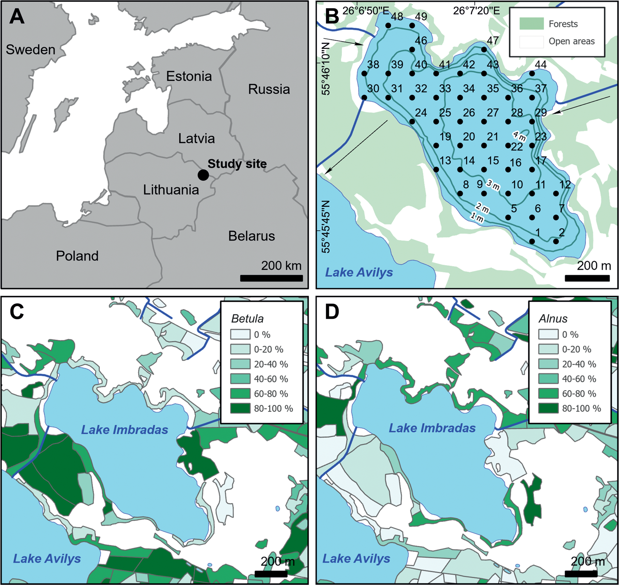
Figure 1. (A) Location of Lake Imbradas; (B) close-up of Lake Imbradas, numbers in lake area indicate locations of the sampling points, arrows indicate direction of water movement into and out of the lake; (C) distribution of Betula and (D) distribution of Alnus vegetation in the surroundings of Lake Imbradas expressed as percentages.
The territory between Lakes Imbradas and Avilys is characterized by dense birch (Betula pendula, B. pubescens; Fig. 1C) and alder (Alnus glutinosa, A. incana; Fig. 1D) forest. The latter is more abundant towards the shore of Lake Imbradas where it becomes one of the dominant tree taxa. A smaller (10 ha) birch-alder fragmented forest is situated on the eastern bank of Lake Imbradas, overlapping the tributary (Fig. 1B). Occasional pine (Pinus sylvestris), spruce (Picea abies), poplar (mainly Populus tremula), and ash (Fraxinus excelsior) trees are observed in both forests. Alder and willow (mainly Salix carpea and S. viminalis) dominate in a narrow belt (<10 m wide) of arboreal vegetation along the shoreline of Lake Imbradas. The main forest-floor taxa are moss (Bryophyta) and peat moss (mainly Sphagnum magellanicum). Grasses (Poaceae), horsetail (Equisetum arvense, E. sylvaticum), wild strawberry (Fragaria vesca), valerian (Valeriana officinalis), and stonecrop (Sedum acre) are also abundant. Open areas are dominated by grazed and un-grazed grasslands. Grasses are by far the most abundant taxon in most meadow and pasture parcels. Umbellifers (mainly Aegopodium podagraria, and Heracleum sibiricum) are moderately represented in most of the parcels and are dominant in several. Dandelion (Taraxacum officinale), speedwell (Veronica arvensis), nettle (mainly Urtica dioica), and raspberry (Rubus idaeus, Rub. caesius) are abundant throughout the study area. Valerian, horsetail, stonecrop, pennywort (Hydrocotyle vulgaris), yarrow (Achillea millefolium), bedstraw (Galium album, G. verum), clover (mainly Trifolium repens and Tr. pratense), plantain (mainly Plantago major), angelica (Angelica sylvestris), buttercup (mainly Ranunculus acris, Ra. repens, and Anemone nemorosa), mallow (Malva neglecta), burdock (mainly Arctium tomentosum), cow parsley (Anthriscus sylvestris), sorrel (mainly Rumex acetosa, and Rum. acetosella), aster (many species of Asteraceae), and primrose (Primula veris) are less frequent. Small patches of bare, arable land are occasionally present in the vicinity of Imbradas village, which is situated 0.5 km northwest from the lake. The banks of Lake Imbradas are overgrown with reeds (Phragmites australis) and bulrush (Typha lafifolia, Ty. angustifolia), especially in the southeastern and northwestern parts of the lake. Water soldiers (Stratiotes aloides), pondweed (Potamogeton perfoliatus, P. natans), watermilfoil (Myriophyllum alterniflorum), frogbit (Hydrocharis morsus-ranae), and water lily (Nymphaea candida) are present towards the center of the lake.
MATERIALS AND METHODS
Fieldwork
Surface sediment samples were collected from locations at the ice-covered lake in March 2018 using a Kajak Model B sediment sampler. This vacuum sampler was specifically designed for lake sediments and does not cause any sediment compaction. The upper 2 cm of sediments were collected for analysis, and we assume that this interval represents sediment deposited during the last 15–40 years based on typical sedimentation rates for Lithuanian lakes (Šeirienė et al., Reference Šeirienė, Kabailienė, Kasperovičienė, Mažeika, Petrošius and Paškauskas2009). This sampling protocol was to ensure that we had representation of sufficient time intervals of at least several years for calculating the average annual variability of pollen deposition, as is standard in surface pollen studies (Bunting et al., Reference Bunting, Farrell, Broström, Hjelle, Mazier, Middleton, Nielsen, Rushton, Shaw and Twiddle2013). The sampling interval of 2 cm was also short enough to exclude the possibility of significant changes in vegetation composition during the represented time interval that would undermine our ability to compare modern vegetation composition and surface pollen data. Sampling locations were arranged in a 110-m rectangular network covering the entire area of the lake (Fig. 1B). Samples 3, 4, 18, and 45 could not be extracted due to dense vegetation on the lake bottom.
Pollen analysis
For this study, 45 surface pollen samples were analyzed. For each sediment sample, 20 cm3 of sediment suspension was prepared following standard laboratory preparation procedures (Berglund and Ralska-Jasiewiczowa, Reference Berglund, Ralska-Jasiewiczowa and Berglund1986). Marker spore tablets with 10,680 Lycopodium clavatum spores in each tablet were added to each sample to enable calculation of pollen concentrations (Stockmarr, Reference Stockmarr1971). Pollen identification and nomenclature followed Moore et al. (Reference Moore, Webb and Collinson1991). Reference slides from the Vilnius University Institute of Geosciences collection were consulted in more complicated cases. Other microfossils were recorded along with the pollen: charcoal particles larger than 25 μm, green algae (Botryococcus, Pediastrum), pine stomata, water flea (Cladocera) remains, as well as bryophyte (Bryophyta) spores. At least 500 terrestrial pollen grains were identified in each sample. Pollen sums were calculated according to Berglund and Ralska-Jasiewiczowa (Reference Berglund, Ralska-Jasiewiczowa and Berglund1986). Terrestrial pollen percentages were calculated based on the main pollen sum (arboreal + non-arboreal pollen). Aquatic, spore, and other microfossil percentages were calculated based on the main pollen sum plus the sum of the corresponding plant group or microfossil. The TILIA program (Grimm, Reference Grimm2011) was used to plot the pollen data. Taxa that constituted at least 0.5% of the pollen sum were presented in the pollen diagram. Pollen analysis results are also presented as maps of total pollen concentrations and pollen percentages, interpolated using the natural neighbor algorithm in ArcGIS Pro software (Esri, 2020). Maps of pollen concentration for individual taxa are not shown because they have patterns similar to those for total pollen concentration given the substantial variation in total pollen concentration across the samples.
Principal component analysis (PCA) was carried out using the ggbiplot package (Vu, Reference Vu2011) in R software (R Core Team, 2020) to explore the main factors influencing pollen assemblages. All pollen taxa with maximum values of at least 1% were included in the PCA.
To visualize the effects of water depth and distance from the lake shore on total pollen concentrations, we generated scatterplots of water depth versus pollen concentration, and distance versus concentration, and calculated Pearson correlation coefficients (r) along with probabilities (p) to evaluate correlations of these variables with pollen concentrations.
The squared chord distance metric (Overpeck et al., Reference Overpeck, Webb and Prentice1985) was used to compare the similarity between pollen assemblages. The square chord distance between samples i and j (di,j) was calculated as follows:

where xi,k is the proportion of taxon k in the sample i, and xj,k is the proportion of taxon k in the sample j. Squared chord distance values range from 0–2, with 0 indicating identical pollen assemblages. This metric was calculated for every pair of sampling locations. Average squared chord distance values between each sampling location and all other sampling locations, as well as between each sampling location and the neighboring locations within a radius of 200 m, were determined to visualize the results. These values were interpolated using the natural neighbor algorithm in ArcGIS Pro software.
Vegetation data
The composition of arboreal vegetation around the lake was evaluated according to the State Forest Cadastre data provided by the Lithuanian State Forest Service. The Cadastre database is constantly updated during the inventory process, registering cut and planted trees, as well as self-seeded trees. Data quality control is ensured by constant remote sensing and surveying campaigns. Information on tree vegetation composition is stored for every parcel at 10% precision. The average size of a forest parcel in the vicinity of Lake Imbradas is 1.2 ha. These data enabled the creation of vegetation maps (Figs. 1C, D; 2; 3C–G; 7), as well as the calculation of absolute arboreal vegetation abundance expressed as canopy coverage area for any of the tree taxa in any selected area.
The radius of the circle in which vegetation composition was evaluated was determined by calculating characteristic radii zɛ(r) (Prentice, Reference Prentice, Huntley and Webb1988). A characteristic radius represents the distance from which the proportion of the pollen (1-ɛ) comes to the basin of radius r and is calculated by:

where γ is a coefficient, equal to 0.125 under typical daytime conditions; bi is a function representing the ratio of the pollen-fall speed (vg) and the effective wind velocity (u): bi = 75 vg/u. Assuming that the radius of a circle of the same area (436 m) can be taken for r at a wind velocity of 3 m/s, and that pollen-fall speed estimates (Table 1) are sufficiently precise, characteristic radii can be calculated for any ɛ of any pollen type.
Table 1. Pollen-fall speed values used in this study: most values from Mazier et al., Reference Mazier, Gaillard, Kuneš, Sugita, Trondman and Broström2012; * = values from Eisenhut, Reference Eisenhut1961.

Simulations in patchy vegetation (Sugita, Reference Sugita1994) showed that reliable estimations of vegetation modeling parameters require a characteristic radius as small as 30–45% (i.e., ɛ value 0.55 to 0.70). Assuming pollen-fall speed values presented in Table 1, and a wind velocity of 3 m/s, the characteristic radii for the various arboreal taxa stored in the forest inventory database range from 0.86 km to 13.28 km (for 1-ɛ = 45%), 0.8 km to 8.7 km (for 1-ɛ = 40%), and 0.7 km to 4.0 km (for 1-ɛ = 30%). Plant abundance (as a proportion of total area) was calculated for the logarithmically increasing concentric rings of outer radii (100 m, 147 m, 215 m, 316 m, 464 m, 681 m, 1000 m, 1468 m, 2154 m, 3162 m, 4641 m, 6813 m, 10,000 m, 14,680 m, and 21,540 m around each of the investigated sites), as well as the centroid of the lake (Fig. 2), thus considerably exceeding the required 30–45% maximum characteristic radius. The three outer radii do not completely fall within the territory of Lithuania (the coverage of our vegetation data). It is, therefore, assumed that vegetation composition is the same outside the evaluated area as it is within the evaluated area. Considering that the unevaluated area is relatively small, this assumption seems reasonable. It should also be noted that the 40% characteristic radius does not reach the unevaluated area in any direction. It was also assumed that the vegetation composition beyond 21,540 m is similar to the average vegetation composition of the evaluated area. In the territory of Lithuania, Pinus makes up 33% of the total forest species, Betula 22%, Picea 19%, Alnus 14%, Populus 6%, Fraxinus 2%, Quercus 2%, and other taxa 2% (Balakauskas, Reference Balakauskas2012). These percentages are similar to those of the main part of the evaluated area (rings of 10,000–21,540 m; Table 2). Therefore, in further calculations, the same vegetation abundance was used beyond the 21,540 m area as the determined average vegetation abundance of the evaluated area.
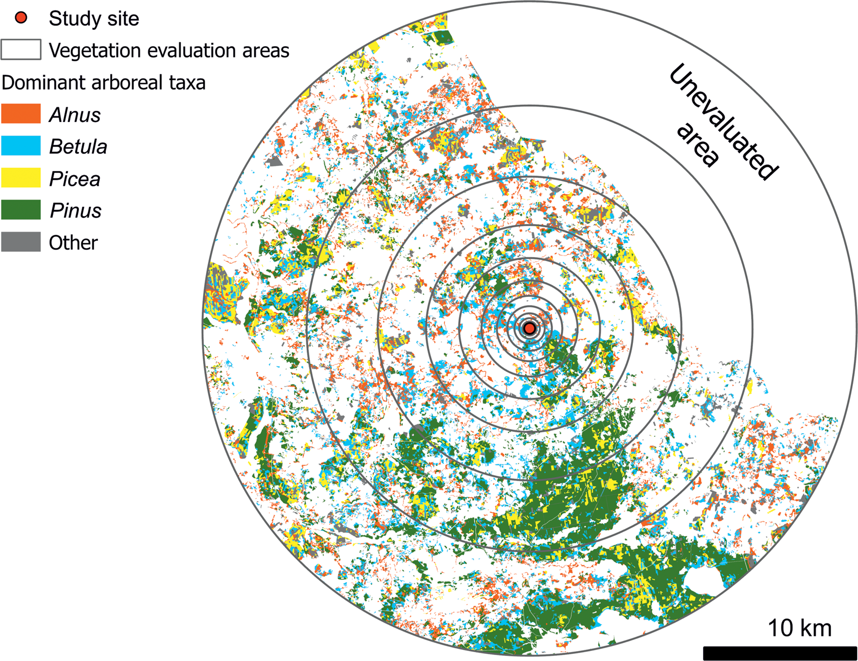
Figure 2. Dominant arboreal vegetation in the surroundings of Lake Imbradas and the areas of evaluation of plant abundance according to the State Forest Cadastre data provided by the Lithuanian State Forest Service. Unevaluated area is outside the Lithuanian border.
Table 2. Percentages of tree vegetation within concentric rings around Lake Imbradas centroid.

The acquired arboreal vegetation data were validated on site in May 2018. Individual trees were counted in 30 × 30 m plots within 10 selected forest parcels and their percentages were compared to those of the vegetation dataset. In addition, the perimeter of the lake edge was visually evaluated for consistency between vegetation in the distinct vicinity of the lake (<10 m from the bank) and the rest of the parcel because such differences were reported earlier when using similar vegetation databases (Balakauskas, Reference Balakauskas2012).
Calculation of pollen productivity
To model the pollen-vegetation relationship in lacustrine environments, the model developed by Sugita (Reference Sugita1993) is usually employed. However, it is not suitable for multiple locations from the same basin because the model averages pollen deposition throughout the lake surface and assumes homogenous pollen assemblages throughout the lake. Therefore, a less complex Prentice (Reference Prentice, Huntley and Webb1988) model that models pollen deposition at a certain point on the ground or water surface can be used. Assuming that pollen transport is not significant after deposition on the lake surface (i.e., vertical deposition dominates), the Prentice (Reference Prentice, Huntley and Webb1988) model can be used to model pollen deposition in sediments at different locations in the same lake. This assumption of insignificant pollen transport after deposition is at least partly fulfilled in the case of Lake Imbradas due to its simple morphology, the absence of significant tributaries, and the consistent, unobscured representation of shoreline vegetation, i.e., pollen percentages decreasing with distance from its source. To validate the performance of the Prentice (Reference Prentice, Huntley and Webb1988) pollen-vegetation relationship model in the environment of Lake Imbradas, pollen productivities were calculated for the main arboreal taxa at every sampling location.
According to the Prentice (Reference Prentice, Huntley and Webb1988) model, for any taxon (i), the relationship between the pollen flux (yi) and distance-weighted vegetation abundance (xi(z)${{{\rm d{\varphi}_i}( {\rm z} ) } \over {dz}}$ dz) can be expressed as pollen productivity (Pi):

where yi is known from the analyzed pollen counts, assuming uniform sedimentation rate throughout the lake (i.e., there is a linear relationship between pollen abundance as expressed in grains per unit of volume, and pollen accumulation rate as expressed in grains per unit of area and time); xi(z) estimation is described above. φ i(z) represents the proportion of pollen that remains airborne within distance z from the source.

where bi is a function of the pollen-fall speed and wind velocity, and γ = 0.125 (see Eq. 2).
Pollen productivity was calculated using Python (van Rossum, Reference van Rossum1995) scripts, according to Eqs. 3 and 4. For comparison with other pollen productivity studies, absolute productivities were converted to relative pollen productivity estimates (PPE). Pinus was chosen as the reference taxon (PPE =1) because it is one of the most abundant and relatively evenly distributed tree taxa throughout the lake sediments, and is widely used as a reference in other pollen productivity studies (Wieczorek and Herzschuh, Reference Wieczorek and Herzschuh2020). The use of Poaceae, more commonly used as a reference taxon, is impossible in this study because it does not appear in the corresponding vegetation data (i.e., our database contains quantitative data on arboreal vegetation only).
The distribution of pollen productivity values was interpolated throughout the lake surface area using the natural neighbor algorithm in ArcGIS Pro software. It should be noted that pollen productivity is not an empirically acquired value. It is, effectively, a ratio between known pollen abundance at a specific location and known distance-weighted plant abundance around that location. Therefore, PPE represents not only the actual differences in pollen productivity between taxa, but also any deviations from model generalizations. A large part of this deviation is site-specific; thus, substantial differences are observed between PPE values obtained in the different regions, or even within the same region (Wieczorek and Herzschuh, Reference Wieczorek and Herzschuh2020). In our case, calculated pollen productivity maps can serve two purposes: 1) they can help to obtain PPE values for vegetation reconstruction at any point of the Lake Imbradas sediment surface, and 2) they validate a pollen-vegetation relationship model in the environment of Lake Imbradas because they are proportional to the ratio between the simulated pollen abundance and the actual pollen abundance as estimated empirically at any point on a map.
RESULTS
Arboreal vegetation of Lake Imbradas surroundings
Within 1 km of the lake, Betula (58–68%) and Alnus (24–33%) dominate (Table 2); Pinus (up to 8%), Picea (up to 2%), Quercus (up to 0.9%), and Populus (up to 0.6%) values are rather low. Outside of a 10 km radius, Pinus and Picea increase to 34–37% and 16%, respectively, at the expense of Betula (23–25%) and Alnus (17–20%). In general, vegetation composition at 10 km and farther is close to the average vegetation composition of Lithuania (Balakauskas, Reference Balakauskas2012). Larix appears at the 4641–6813 m interval, although in negligible amounts that do not exceed 0.1% at any radius. Most deciduous tree taxa (Fraxinus, Tilia, Acer, Salix, Ulmus, Carpinus) appear more than 1 km from the lake centroid, although they do not exceed 1% at any distance interval. Exceptions to this are Populus and Quercus, appearing at 681–1000 m with less than 1%, increasing to 3–5% and more than 1% at farther distances, respectively.
Validation of the vegetation dataset in the field showed that the actual plant abundance percentages (rounded to 10% in the same way they are rounded in the forestry database) are identical to those of the vegetation database in all ten validated parcels. However, near the lakeshore, and up to several meters away, representation of Alnus appeared considerably higher than that recorded in the forestry database at most locations. Also, a considerable amount of Salix trees were identified within several meters of the lake bank, but this taxon is supposed to be absent within 1468 m of the lake center according to the forestry database. It should be noted that the forestry database does not include self-seeded trees near the lake bank, nor trees significantly lower than canopy level because these do not present economic value. However, self-seeded trees near the lake bank constitute only a very small portion of the total parcel of trees and thus do not affect the rounded values of a parcel, while trees significantly lower than canopy level do not have a significant influence on airborne pollen composition due to the difficulty in overcoming the canopy barrier (Tauber, Reference Tauber1965). The exception to this is trees growing close (<10 m) to the lake bank outside forest parcels; influence of these trees on lake pollen data could be considerable because a large proportion of their pollen falls directly into the lake.
Pollen assemblages of Lake Imbradas sediments
Pollen concentrations (Figs. 3A, 4) proved to be the highest (161,482 grains/cm3) southwest from the center of the lake, gradually decreasing towards the lake bank, where pollen concentrations are 2–5 times lower. The exceptions to this were samples 36 and 47, where concentrations were up to approximately 90,000 grains/cm3.

Figure 3. (A) Pollen concentration; (B–K) pollen percentages; and (L) spore percentages in Lake Imbradas surface sediments. Green areas show forests; in cases when the corresponding vegetation abundance is known (C–G), quantitative taxon abundance is shown in gray shading instead.

Figure 4. Pollen diagram for Lake Imbradas surface sediments.
Arboreal pollen (AP) constitutes 71–91% and is most abundant in the central part of the lake, gradually decreasing towards the lake bank (Fig. 3B). Betula (Fig. 3C) and Alnus (Fig. 3D) are among the dominant pollen types, reaching 28–43% and 8–14%, respectively. Higher values of these taxa are characteristic of not only the center of the lake, but also in some places nearer to the banks of the lake, along the forests of the corresponding vegetation. Pinus values (20–30%; Fig. 3E) are highest in the eastern and northern parts of the lake. Quercus values reach 3% (Fig. 3F) and are highest in the center of the lake, and gradually decrease towards the shoreline. Salix (up to 2%; Fig. 3G) is the most abundant along the forested shores, peaking less markedly in the central part of the lake. The percentages of Poaceae (4–17%) and Cyperaceae (up to 3%) are the highest along the unforested shores of the lake (Fig. 3H, I). Aster type (up to 0.3%), although having low values throughout the lake, obviously increases towards the lake shore, while no pollen of this type was identified at many locations in the center of the lake (Fig. 3J). Rumex acetosa/acetosella (Fig. 3K) demonstrates a similar pattern of distribution, although with larger quantities (up to 4%). Polypodiaceae (1–7%; Fig. 3L) significantly increases in the southeastern part of the lake along the forested area.
PCA analysis of the pollen data (Fig. 5) showed that Betula, Quercus, Corylus, Alnus, Picea, and Salix have positive values on the maximal variance axis (PC1), while other, mostly non-arboreal taxa have negative values. Values on the second-highest axis of variance (PC2) are largest for Pinus, Picea, and other taxa poorly represented in shoreline vegetation (i.e., parcels facing the lake bank) but relatively abundant as background vegetation (defined as growing roughly >200 m from the lake bank). The lowest PC2 values are for Alnus, Betula, Salix, and many non-arboreal taxa with high shoreline:background ratios.

Figure 5. PCA analysis results for Lake Imbradas surface sediments.
Squared chord distance analysis shows that pollen assemblages are relatively homogenous throughout the lake, with average values in the 0.05–0.1 range for a large area of the basin. Homogeneity is especially the case for the center of the lake where water depth is >3 m, and in the eastern part of the lake (locations 14, 19, 24, 25, 30, 31, 32, 39, and 40). Average squared chord distances increase towards the shore of the lake, reaching 0.23 at the location 1. When compared to neighboring locations within 200 m radii, average squared chord distance values range from 0.03 to 0.14, and lower values are also common in the central part of the lake.
Pollen concentrations increase with distance from the shore (r = 0.48; p<0.001), but they appear to be less correlated with lake depth (r = 0.34; p = 0.024). The most prominent outlier in scatterplots for these relationships (Fig. 7A, B) is location 20, which has an exceptionally high pollen concentration.

Figure 6. Average squared chord distances (SCD) for pollen assemblages from Lake Imbradas surface sediments (A) between a location and all other locations, and (B) between a location and neighboring locations within 200 m radius.

Figure 7. Scatterplots for Lake Imbradas pollen data: (A) pollen concentrations versus distance to the shore; (B) pollen concentrations versus water depth. Solid lines represent best-fit correlations.
Distribution of pollen productivity estimates
The calculated Betula (Fig. 8A) productivity (in relation to the reference taxon Pinus) ranges from approximately 1 in the northern and eastern parts of the lake, to 2 in the southeastern part of the lake. The calculated productivity of Alnus (Fig. 8B) distribution is very similar, ranging from approximately 0.4 in the northern and eastern parts of the lake to 0.7 in the southeastern part of the lake. Picea (Fig. 8C) values tend to be lower (around 1) near the banks of the lake, increasing to approximately 2.5 in the central part of the lake. However, samples 32, 34, and 16 demonstrate low Picea productivities despite their central location. Quercus (Fig. 8D), Fraxinus (Fig. 8E), and Ulmus (Fig. 8F) have their highest values around locations 19, 20, 21, 25, and 33. The productivity range of these taxa is far wider, which is expected considering their low pollen abundances and potentially higher error. Tilia (Fig. 8G) values are lower (around 0.5) near the center of the lake, increasing to 2.0–2.5 towards the edges. Salix (Fig. 8H) productivities range from 2–11 and are somewhat higher in the central part of the lake. The highest Salix values, however, are generally along the forested edges of the lake. The distribution of Populus productivity values (Fig. 8I) is the most irregular, ranging from 0.06–0.30. Productivities of other arboreal taxa are not discussed here due to their extremely low representation in the surrounding vegetation and/or pollen assemblages.

Figure 8. Distribution of the calculated pollen productivity for arboreal taxa in the surface sediments of Lake Imbradas.
DISCUSSION
Variation of pollen concentration and percentages throughout the lake
Surface sediments from Lake Imbradas show significant spatial variation in pollen concentration. In theory, a lake surface should receive about the same total terrestrial pollen influx from the background vegetation (i.e., vegetation growing >200 m from the lake; mainly comprising the rain component: Tauber, Reference Tauber1965) across its surface. The intra-lake vegetation does not contribute to the terrestrial pollen influx because it is mainly composed of aquatic taxa. Thus, the only vegetation that can cause considerable variance of the terrestrial pollen influx throughout the lake is vegetation growing along the shoreline of the lake. This component of pollen primarily depends on the pollen production and transport in the immediate vicinity of the lake. Therefore, the pollen influx originating from the shoreline vegetation and, consequently, the total terrestrial pollen influx, should be highest near the shoreline of the lake because it is closer to the source (Prentice, Reference Prentice, Huntley and Webb1988; Sugita, Reference Sugita1993). Thus, in theory, the edges of the lake should receive more pollen grains than the center. In the case of Lake Imbradas, the distribution of pollen concentrations is reversed, with the highest pollen concentrations in the central part of the lake. Such a distribution has been observed in other lakes (Davis et al. Reference Davis, Brubaker and Beiswenger1971; Huang et al., Reference Huang, Zhou, Ma, Xu and Chen2010) and appears to be related to differences in sedimentation rate. Recent lithological analyses of Lake Imbradas (Balakauskas et al., Reference Balakauskas, Vaikutienė, Paškevičiūtė, Valskys and Spiridonov2021) showed that higher amounts of mineral and carbonate matter accumulate near the edges of the lake. This matter adds significant sediment volume, thus reducing the pollen concentration (pollen grains per volume of sediment) in these areas. Apparently, the effect of more rapid sedimentation near the shoreline and decreasing pollen concentration overwhelms the effect of higher pollen influx in these areas. It could therefore be argued that the sedimentation rate near the edges of Lake Imbradas must be higher than, or is at least as high as, the differences in pollen concentration between these areas (i.e., the sedimentation rate should be at least two to five times higher near the shoreline, compared to the central part of the lake).
Only slight differences in pollen concentrations are observed near the mouths of the main tributaries, which, along with low discharges, suggest only a minor influence of the tributaries on the spatial distribution of pollen in Lake Imbradas. Two areas that deviate from the symmetry of the pollen concentration distributions occur along the northern bank around locations 36 and 47. The higher concentrations in these areas could be related to the discharge from the tributaries: location 36 receives inflow from the main tributary from the east, whereas location 47 could experience inflow from the unmapped tributary (discharging ~5 l/s), situated in close proximity to the site. On the other hand, lower pollen concentrations in these areas (at locations 29, 34, 37, 42, and 46) could result from larger volumes of sediment originating from macrophyte production, thus decreasing pollen concentrations in these areas. These hypotheses should be tested by further investigations. Whatever the reason for these differences in pollen concentrations, these areas are extremely limited in their spatial extent. Thus, tributaries do not seem to affect pollen distribution throughout Lake Imbradas to any great degree.
It is also unlikely that turbulence played an important role in the redistribution of pollen after reaching the water surface because the intralake (aquatic) and shoreline vegetation is consistently represented in the surface pollen record. Because lakes in Lithuania are dimictic (mixing twice a year), resuspension processes can occur to some extent (Kilkus, Reference Kilkus2000). However, this process is more significant in deep lakes with a complex bottom morphology, while Lake Imbradas is shallow, with a simpler, gradually sloped bottom morphology that prevents resuspension as well as the transportation of sediment downslope.
In Lake Imbradas (and possibly other flat-bottomed lakes), pollen concentration is more strongly correlated with distance to the shore than with depth, which suggests that sedimentation rate and sediment input are more important factors than lake-bottom morphology. The most prominent outlier in the concentration versus distance to the shore scatterplot (Fig. 5) is sample 20, which also has the highest pollen concentration. The decrease in concentrations is gradual in all directions from this location, that is, values are spatially consistent. At this location, the organic, carbonate, and mineral matter contents are very similar to those of the surrounding locations (Balakauskas et al., Reference Balakauskas, Vaikutienė, Paškevičiūtė, Valskys and Spiridonov2021), which does not suggest particularly slow sedimentation at this site in relation to other central sampling locations. Accordingly, a high pollen concentration at location 20 cannot be justified merely by differences in sedimentation rate. Interestingly, the same location has the most homogenous diatom assemblages in relation to the other analyzed locations (Balakauskas et al., Reference Balakauskas, Vaikutienė, Paškevičiūtė, Valskys and Spiridonov2021). It is neither the deepest nor the most central part of the lake. The deepest part (4.08 m) of the lake is at location 22, while the locations lying closest to the lake centroid (situated between samples 20, 21, 26, and 27) are 21 and 27 (both ~64 m from the centroid). Exceptionally high pollen concentrations at this location may arise from the hydrodynamics of the lake. Because the inflow and outflow direction are southwestward, sediments may be redistributed from northeast to southwest; this slow process would concentrate the smallest sedimentary particles (Sly, Reference Sly and Lerman1978), including pollen grains. This process may be reinforced by a spring source at the bottom of Lake Imbradas between sampling points 22, 23, and 29 that increases sedimentation rates towards the central part of the lake. In any case, because location 20 is the pollen-focusing point (highest pollen concentration) with the highest representation of the background taxa (i.e., mostly arboreal pollen), it seems to be the optimal sampling location for reflecting the regional pollen rain. This conclusion assumes that the lake hydrodynamics did not change considerably throughout the investigated time interval. Although location 33 has the highest representation of background taxa, the pollen assemblage is not spatially consistent with the surrounding locations; such inconsistencies might arise due to sediment disturbance. Therefore, it would be safer to avoid this location for sampling.
It should be emphasized that pollen assemblages in the surface sediments of Lake Imbradas are similar to each other, especially in the central part of the lake. For example, the squared chord distance between location 20 and the deepest location (location 22) is 0.029, and squared chord distances between location 20 and the central locations 21 and 27 are 0.026 and 0.072, respectively. If we assume that low heterogeneity in pollen deposition prevailed in the lake during the investigated period, any coring location lying >200 m from the shore should be fairly representative, and likely would not affect the conceptual interpretation noticeably. Nevertheless, when higher precision is required (e.g., in quantitative past-vegetation reconstructions), acknowledgement of even small spatial variation can be important.
The PC1 axis largely represents the background significance of different taxa. Arboreal pollen (AP) taxa, abundant outside the shoreline area (especially Quercus, Corylus, Betula, and Alnus), have the highest PC1 values, while herbs, abundant along the shoreline (Rumex, Poaceae, Cyperaceae, and Artemisia) have the lowest values. High PC1 taxa have higher values in the central part of the lake where they are not overwhelmed by the shoreline taxa. The ability of a sampling location to represent regional vegetation seems to be the most important factor determining variations in pollen composition in Lake Imbradas sediments.
The PC2 axis, on the other hand, could be related to the absence of certain taxa along the shoreline. Taxa with high PC2 values are abundant in the background vegetation but are absent along the shoreline (e.g., Picea, Tilia, and Quercus) or less abundant than their background levels (e.g., Pinus). In contrast, taxa with low PC2 values grow along the margin of the lake (<10 m from the shore). Betula and Alnus are dominant in the forests facing the lake bank. Salix, although absent in the forestry data, is fairly abundant in the self-seeded shoreline vegetation. Similarly, most of the shrub and herb taxa with negative PC2 values were observed in the nearby meadows, pastures, and forests. Cultivated taxa (e.g., Cerealia, Secale cereale) were not observed in vegetation surveys, but their cultivation is possible in arable fields around Imbradas village.
Most of the background taxa (i.e., high PC2 values) feature relatively low percentage ranges. Because their influx should be more or less uniform throughout the lake's surface (Davis et al., Reference Davis, Brubaker and Beiswenger1971), most of the spatial variation in their percentages could be explained by the so-called Fagerlind (Reference Fagerlind1952) effect, i.e., variations in the influx of shoreline pollen, constituting the same pollen sum. This also explains the similar distribution of different background taxa: they peak in locations where the values of the most abundant shoreline taxa are decreased.
In contrast, shoreline taxa differ considerably in their rates of decreasing pollen abundance with distance from their pollen source. These relationships are generally known for arboreal taxa from existing vegetation data, whereas for herbs, the source vegetation is simply presumed to be situated inland at the location of each taxon's highest surface-pollen value. For instance, Betula and Alnus (having a significant background component) decrease less dramatically with distance from the source (approximately 42% to 35%, and 13% to 11% within 300 m of their highest value location, respectively). Taxa that have a weaker background signal (predominantly less abundant herbs and spores) decrease more markedly (Cyperaceae 3% to 1%, Rumex 4% to 1%, and Polypodiaceae 7% to 2% within 300 m from their highest value). Taxa with the steepest distance gradients (e.g., Aster type) disappear completely or almost completely within a certain distance from their source. Such quantified distance gradients could be used in fossil studies in the same lake or similar nearby lakes for the localization of source vegetation and validation of ring source modeling results, ideally involving several cores from the same basin. Distance gradient data from other localities could enable a more universal use of this approach. However, high-resolution spatial investigations of surface pollen that would enable distance gradient calculation are still extremely rare (Huang et al., Reference Huang, Zhou, Ma, Xu and Chen2010).
Spatial analysis of surface pollen data can also facilitate site selection by locating areas most sensitive to the investigated phenomenon. In traditional single-core studies, coring is usually carried out in the central or deepest location (Larsen and MacDonald, Reference Larsen and MacDonald1993). Central locations are less prone to the undesirable effect of differential deposition (Beaudoin and Reasoner, Reference Beaudoin and Reasoner1992) and are less influenced by minor shoreline pollen types (Davis et al., Reference Davis, Brubaker and Beiswenger1971). In lakes with cone-shaped bottoms, where basin morphology exerts a stronger control over sediment accumulation, the deepest location might be preferred (Lehman, Reference Lehman1975). When GPR measurements or extensive coring data are available, the location of the thickest sediment might be chosen. None of these approaches, however, consider the spatial heterogeneity of pollen assemblages in the lake. Attempts that were made to apply a simulation approach for considering the surrounding vegetation in the process of site selection have been unsatisfactory (von Stedingk and Fyfe, Reference von Stedingk and Fyfe2009).
Considerations regarding spatial variation of pollen productivity
Pollen productivity is a crucial variable in quantitative vegetation reconstructions, and it is usually estimated from modern pollen and vegetation percentage data (Wieczorek and Herzschuh, Reference Wieczorek and Herzschuh2020) according to pollen-vegetation relationship models, similar to the one used in our study (Prentice, Reference Prentice, Huntley and Webb1988; Sugita, Reference Sugita1993). Regional differences in PPEs are widely known (Broström et al., Reference Broström, Nielsen, Gaillard, Hjelle, Mazier, Binney and Bunting2008; Mazier et al., Reference Mazier, Gaillard, Kuneš, Sugita, Trondman and Broström2012; Wieczorek and Herzschuh, Reference Wieczorek and Herzschuh2020), and our findings suggest that to model the pollen-vegetation relationship precisely, different pollen productivity values would have to be used, even for different locations in the same basin (Fig. 8).
Squared chord distance analysis shows that pollen assemblages are rather homogenous throughout the lake. Although these differences have undoubtedly influenced the simulated PPE values, the differences between pollen assemblages are far too low to explain differences between the simulated PPE values. Because the sampling locations in Lake Imbradas share similar source vegetation, larger differences in PPE values from the same basin can only be caused by inaccurate pollen abundance estimates, vegetation data, and/or pollen dispersal functions (Sugita, Reference Sugita1994). While estimation of vegetation abundance and pollen composition is never completely precise, it is rarely a significant source of error in the estimation of pollen productivity (Broström et al., Reference Broström, Nielsen, Gaillard, Hjelle, Mazier, Binney and Bunting2008; Baker et al., Reference Baker, Zimny, Keczyński, Bhagwat, Willis and Latałowa2015). The shortcomings and numerous assumptions made in pollen dispersal functions, on the other hand, are widely known and should always be considered (Sugita, Reference Sugita1994; Theuerkauf et al., Reference Theuerkauf, Kuparinen and Joosten2012). Another source of PPE estimation error could arise from using pollen concentration data and assuming a linear relationship between pollen concentration and pollen accumulation rate, thus skewing the pollen abundance component used by the model. A linear relationship between pollen concentration and pollen accumulation rate is clearly not the case in Lake Imbradas. If stable conditions for the lake are assumed, which is probable throughout the post-glacial period, considering the simple shape of the lake and the minor influence of the tributaries on hydrodynamics and sedimentation, even biased PPE values (calculated at a sampling location) can be used for vegetation reconstructions at that particular sampling location. The vast majority of pollen productivity estimates (Broström et al., Reference Broström, Nielsen, Gaillard, Hjelle, Mazier, Binney and Bunting2008; Mazier et al., Reference Mazier, Gaillard, Kuneš, Sugita, Trondman and Broström2012; Baker et al., Reference Baker, Zimny, Keczyński, Bhagwat, Willis and Latałowa2015) are based on pollen concentrations (as in our study) or on pollen percentages. The latter presents even more challenges, such as the necessity to use Extended R-value (ERV) models (Parsons and Prentice, Reference Parsons and Prentice1981; Prentice and Parsons, Reference Prentice and Parsons1983; Sugita, Reference Sugita1994) to eliminate the Fagerlind effect (Fagerlind, Reference Fagerlind1952). Despite these challenges, these PPE values are used successfully for vegetation and landscape reconstructions (Gaillard et al., Reference Gaillard, Sugita, Bunting, Middleton, Broström, Caseldine and Giesecke2008; Reference Gaillard, Sugita, Mazier, Trondman, Broström, Hickler and Kaplan2010; Trondman et al., Reference Trondman, Gaillard, Mazier, Sugita, Fyfe, Nielsen and Twiddle2015). Thus, using pollen concentrations can present an effective alternative to pollen accumulation rates because acquiring modern pollen accumulation rate data directly is extremely time consuming, requiring several years of pollen influx monitoring (Hicks, Reference Hicks2001). Furthermore, the use of pollen accumulation rates presents an additional set of problems, for example, differences between pollen influx to pollen traps and influx to actual sediments (Xu et al., Reference Xu, Tian, Bunting, Li, Ding, Cao and He2017) must be taken into account.
Most relative pollen productivities calculated at the Lake Imbradas sampling locations are comparable to PPE values reported from elsewhere in Europe (Wieczorek and Herzhuh, Reference Wieczorek and Herzschuh2020), recalculated using Pinus as a reference taxon. However, Betula and Alnus productivities are relatively high in Lake Imbradas sediments. This suggests that arboreal vegetation that is abundant along the shoreline is underrepresented by the pollen dispersal function in Lake Imbradas. Due to the higher sedimentation rate at locations along the forested shores of the lake where these taxa are the most abundant, pollen concentrations of these taxa should be lowered, thus decreasing the calculated pollen productivity at these locations. Despite this, calculated productivities are increased in these areas, i.e., the pollen-vegetation model underestimated shoreline vegetation strongly enough to compensate for the effect of lowered pollen concentrations arising due to more rapid sedimentation. Similar model behavior has been observed in the dense forests of Poland (Baker et al., Reference Baker, Zimny, Keczyński, Bhagwat, Willis and Latałowa2015), where all arboreal forest taxa PPEs were extremely high.
Pinus is dominant among the background vegetation but extremely scarce along the shoreline and accordingly, seems to be overestimated. This reduces all other relative productivity values that were calculated according to Pinus. Most of the background deciduous trees have values similar to average European PPEs or even lower. They are all higher near the center of the lake, which also shows higher representation in this area by the dispersal model, opposite to what is observed in the shoreline taxa. Underrepresentation is also evident in the case of Salix. In other European studies (Wieczorek and Herzhuh, Reference Wieczorek and Herzschuh2020), Salix PPE does not exceed 0.46 in relation to Pinus. In Lake Imbradas, however, it varies between approximately 2 and 11. Although its parent vegetation is not represented in the forestry database, the calculated productivity values are most likely elevated by the occasional Salix trees growing on the lake bank, observed during fieldwork. The underestimation of lakeshore vegetation by the main pollen dispersal models has already been noted in Lithuania (Balakauskas, Reference Balakauskas2012) and elsewhere (Broström et al, Reference Broström, Nielsen, Gaillard, Hjelle, Mazier, Binney and Bunting2008; Baker et al, Reference Baker, Zimny, Keczyński, Bhagwat, Willis and Latałowa2015).
This finding might indicate the need to adjust pollen dispersal models to better represent shoreline vegetation, although this observation should be confirmed by further investigations from other environments, preferably using well-refined pollen accumulation data. Thus far, the above-mentioned indications are only valid for Lake Imbradas and similar lakes in similar environments. When following the traditional approach of single-core fossil pollen studies, these possible shortcomings are less evident due to simplification by treating the whole basin as a single point, rather than a complex sedimentation system. Although pollen-vegetation relationship models provide a solid basis for past vegetation reconstructions, they rely on many assumptions, and the need for validation in real-world environments is widely stressed (Sugita, Reference Sugita1994; Hellman et al., Reference Hellman, Gaillard, Broström and Sugita2008). Furthermore, these models were never meant to consider the heterogeneity of pollen assemblages within the lake (Sugita, Reference Sugita1993) because they are mainly utilized for regional vegetation and landscape reconstructions. To adopt these models for use at particular points of a lake sediment surface, more high-resolution spatial pollen studies are necessary to highlight the factors affecting the heterogeneity of pollen assemblages in a lake.
CONCLUSIONS
Pollen concentrations are highest in the central part of Lake Imbradas, largely due to the lower sedimentation rate compared to areas near the lakeshore. Differences in pollen concentrations at different locations in the lake can therefore provide a rough estimate of sedimentation rates across the lake. Spatial variability of pollen in the sediments of Lake Imbradas is rather low. Minor differences in pollen assemblages arise from variations in the pollen contributions from shoreline and background vegetation. The effects of tributaries, redeposition, and mixing are relatively weak, which suggests that the vegetation signal in pollen assemblages is fairly unobscured. Background pollen tends to have higher values in the central part of the lake, while shoreline taxa percentages gradually decrease with distance from their pollen source. The gradient of this decrease depends on the background significance and dispersal properties of an individual taxon.
Due to the low heterogeneity of pollen assemblages in the central part of the lake, any location within this area (including the centroid, depocenter, and deepest locations) should be fairly suitable for conventional single-core fossil studies, and site selection is unlikely to affect the conceptual interpretation of such data to a noticeable extent. However, our study demonstrates that even low variations in pollen assemblages can significantly impact PPE values, thus leading to higher errors of quantitative vegetation reconstructions. Our results also suggest that the Prentice pollen dispersal model (Prentice, Reference Prentice, Huntley and Webb1988) underestimates the importance of shoreline vegetation in Lake Imbradas, especially that of arboreal vegetation growing in close proximity to the lake. Similar investigations in other lakes with different morphologies and environmental settings could reveal possible systematic drawbacks of pollen dispersal functions, thus facilitating their development.
Absolute pollen abundance values, acquired from detailed surface pollen studies and combined with detailed vegetation data, provide the opportunity to efficiently validate pollen-vegetation relationship models for use in a particular basin without the necessity of carrying out time-consuming vegetation surveys and using ERV models. Pollen productivity estimates calculated from known modern pollen and vegetation abundances can be used directly in quantitative vegetation reconstructions at the same points for which they were calculated, thus enabling multi-core quantitative paleovegetation reconstructions. This assumes that the environmental conditions of the lake basin remained stable throughout the investigated time interval. However, pollen percentage and concentration data should be interpreted with care because their use requires an assumption of even sedimentation rates throughout the basin, which is not the case in most real-world environments. Ideally, pollen accumulation rate data should be used to address this issue.
High-spatial-resolution modern pollen studies in combination with evaluation of heterogeneity of pollen assemblages, present valuable context for site selection and fossil data interpretation (both conceptual and quantitative), providing additional spatial dimensions by area instead of a point. An optimal coring location or area for regional reconstructions might be selected by using modern pollen data to locate a focusing point for regional pollen. Modern pollen data also facilitate studies of local phenomena by delineating locations where pollen records are most sensitive to these phenomena. For example, distance gradients of shoreline taxa can be used on fossil pollen data to evaluate the proximity of an investigated point to the nearest source vegetation of the selected taxa. Using a multi-core approach, arranging cores at different distances and/or angles from an area of interest could yield the approximate location of fossil pollen sources. Of course, when choosing sampling locations for fossil studies following this approach, an assumption has to be made that the shape and hydrodynamics of the lake have been stable throughout the investigated time interval. Extrapolating insights from the Lake Imbradas data on site selection to other lakes is extremely problematic due to possible differences in lake size, shape, bathymetry, tributaries, and surrounding vegetation, etc. Therefore, we propose that investigators should carry out a similar modern pollen study prior to fossil investigations in cases when such information is necessary and data from other studies do not allow extrapolation, such as in high-precision fossil studies, and particularly those involving quantitative vegetation reconstructions.
Supplementary Material
The supplementary material for this article can be found at https://doi.org/10.1017/qua.2021.51
Acknowledgments
The authors are sincerely grateful to Professor Sigitas Radzevičius and Robertas Žeglaitis for their help during the fieldwork, as well as to the anonymous reviewers for valuable remarks and ideas concerning pollen-vegetation relationship modeling and site selection. We are also grateful to the staff of Proof-Reading-Service.com for proofreading the paper.


