1 Introduction
The study of gravity- and surface-tension-driven oscillations at the interface of two immiscible fluids, on quiescent base states described by Cartesian, cylindrical or spherical geometries, were amongst the earliest analytical studies on interfacial waves. Most of the early results came from studies by Poisson (Reference Poisson1818), Cauchy (Reference Cauchy1827), Kelvin (Reference Kelvin1871, Reference Kelvin1887), Rayleigh (1879), Stokes in 1880 (see Stokes Reference Stokes2009), Korteweg & De Vries (Reference Korteweg and De Vries1895), Wilton (Reference Wilton1915) and Lamb (Reference Lamb1932). Many of these investigations were in the linearised, inviscid, irrotational approximation (for studying free oscillations) and led to what are now considered, classical dispersion relations, e.g. the capillary–gravity dispersion relation in deep water by Kelvin (Reference Kelvin1871) obtained in Cartesian geometry, the dispersion relation for oscillations of a liquid sphere obtained using spherical coordinates (Rayleigh 1879; Lamb Reference Lamb1932), the Rayleigh–Plateau (RP hereafter) dispersion relation for a cylindrical filament (Plateau Reference Plateau1873; Rayleigh 1879) etc. Despite the apparently restrictive assumption of linearity along with irrotationality, these inviscid relations have played an important role in understanding instabilities of viscous, long fluid filaments (Driessen et al. Reference Driessen, Jeurissen, Wijshoff, Toschi and Lohse2013), instabilities on coated fibres (Haefner et al. Reference Haefner, Benzaquen, Bäumchen, Salez, Peters, McGraw, Jacobs, Raphaël and Dalnoki-Veress2015), controlling jet breakup (Driessen et al. Reference Driessen, Sleutel, Dijksman, Jeurissen and Lohse2014), understanding various modes of oscillation of falling rain drops (Testik, Barros & Bliven Reference Testik, Barros and Bliven2006) and for measuring surface tension (Rayleigh 1890). These inviscid relations have also proven useful for understanding energy transfer due to resonant interactions among gravity/capillary–gravity waves (Phillips Reference Phillips1960; Longuet-Higgins Reference Longuet-Higgins1962; McGoldrick Reference McGoldrick1965) and internal resonance in droplet oscillations (Natarajan & Brown Reference Natarajan and Brown1987).
Viscous extensions of these relations have also been reported. In Cartesian coordinates, the viscous extension was obtained by Harrison (Reference Harrison1908). For a spherical droplet, it was derived by Miller & Scriven (Reference Miller and Scriven1968) (also see Lamb (Reference Lamb1932) and Prosperetti (Reference Prosperetti1980)). For the cylindrical filament, viscous corrections to the RP dispersion relation were introduced by Rayleigh (1892) and Bohr (Reference Bohr1909) (also see Tomotika (Reference Tomotika1935), Stone & Brenner (Reference Stone and Brenner1996) and table 1 in Ashgriz & Mashayek (Reference Ashgriz and Mashayek1995)). These viscous relations have also been tested, numerically and experimentally. Using direct numerical simulations (DNS), the viscous capillary/capillary–gravity dispersion relation in Cartesian and cylindrical geometries was validated by Denner (Reference Denner2016) and Farsoiya, Mayya & Dasgupta (Reference Farsoiya, Mayya and Dasgupta2017), respectively. The study by Denner (Reference Denner2016) used a damped harmonic oscillator model to study the dispersion of capillary waves, reporting good agreement. The Miller & Scriven (Reference Miller and Scriven1968) viscous relation in spherical geometry has been validated experimentally by Trinh, Zwern & Wang (Reference Trinh, Zwern and Wang1982) and Basaran, Scott & Byers (Reference Basaran, Scott and Byers1989). The viscous RP dispersion relation was validated using DNS by Popinet (Reference Popinet2009), Cervone, Manservisi & Scardovelli (Reference Cervone, Manservisi and Scardovelli2010).
The study of parametrically forced interfacial oscillations, started with observations by Michael Faraday (see appendix in Faraday et al. (Reference Faraday1837)). Here too, the first theoretical analysis by Benjamin & Ursell (Reference Benjamin and Ursell1954) assumed linearised inviscid, irrotational flow, demonstrating that the amplitude of a spatial (Fourier or Bessel) mode is governed by the Mathieu equation. The known properties of Mathieu functions led Benjamin & Ursell (Reference Benjamin and Ursell1954) to obtain the amplitude of forcing
 $h$
at which the (flat) interface becomes linearly unstable to a standing wave of wavenumber
$h$
at which the (flat) interface becomes linearly unstable to a standing wave of wavenumber
 $k$
, for a given forcing frequency
$k$
, for a given forcing frequency
 $\unicode[STIX]{x1D6FA}$
. A stability chart constructed on the amplitude of forcing versus wavenumber (
$\unicode[STIX]{x1D6FA}$
. A stability chart constructed on the amplitude of forcing versus wavenumber (
 $h$
–
$h$
–
 $k$
) plane shows tongue shaped curves. For sufficiently small forcing amplitude, choosing parameters corresponding to values inside the tongues implies a frequency response of the surface (with exponential growth) of
$k$
) plane shows tongue shaped curves. For sufficiently small forcing amplitude, choosing parameters corresponding to values inside the tongues implies a frequency response of the surface (with exponential growth) of
 $n\unicode[STIX]{x1D6FA}/2$
with
$n\unicode[STIX]{x1D6FA}/2$
with
 $n=1,2,3\ldots$
(Benjamin & Ursell Reference Benjamin and Ursell1954), labelled as subharmonic and harmonic alternately. Outside these tongues for finite forcing amplitude
$n=1,2,3\ldots$
(Benjamin & Ursell Reference Benjamin and Ursell1954), labelled as subharmonic and harmonic alternately. Outside these tongues for finite forcing amplitude
 $h$
, a standing wave perturbation produces a bounded, oscillatory (but not necessarily periodic) response (Benjamin & Ursell Reference Benjamin and Ursell1954). An important extension of Faraday waves to spherical base state geometry has been made recently by Adou & Tuckerman (Reference Adou and Tuckerman2016), who show that in this geometry the inviscid problem is also governed by a Mathieu equation whose coefficients depend only on the lower index
$h$
, a standing wave perturbation produces a bounded, oscillatory (but not necessarily periodic) response (Benjamin & Ursell Reference Benjamin and Ursell1954). An important extension of Faraday waves to spherical base state geometry has been made recently by Adou & Tuckerman (Reference Adou and Tuckerman2016), who show that in this geometry the inviscid problem is also governed by a Mathieu equation whose coefficients depend only on the lower index
 $l$
of the spherical harmonic
$l$
of the spherical harmonic
 $Y_{l}^{m}(\unicode[STIX]{x1D703},\unicode[STIX]{x1D719})$
. Extension of these inviscid results to the viscous case has been made in both Cartesian and spherical geometries (Kumar & Tuckerman Reference Kumar and Tuckerman1994; Kumar Reference Kumar1996; Adou & Tuckerman Reference Adou and Tuckerman2016), where using Floquet theory, it has been demonstrated that it is possible for the first unstable response to be harmonic rather than subharmonic. A comprehensive review of Faraday waves and associated parametric instability prior to 1990 and 1989–2000 is given by Miles & Henderson (Reference Miles and Henderson1990) and Perlin & Schultz (Reference Perlin and Schultz2000), respectively (also see DNS studies by Wright, Yon & Pozrikidis (Reference Wright, Yon and Pozrikidis2000), O’Connor (Reference O’Connor2008), Perinet, Juric & Tuckerman (Reference Perinet, Juric and Tuckerman2009)). In addition to witnessing substantial theoretical progress, the subject of interfacial parametric instabilities has also seen applications in vibration-induced atomisation (James et al.
Reference James, Vukasinovic, Smith and Glezer2003), leading to novel technologies for nebulisation (Tsai et al.
Reference Tsai, Mao, Lin, Zhu and Tsai2014). From a theoretical perspective, variable separability of the solutions to the Laplace equation in rectangular, spherical and cylindrical coordinates suggests the possibility of a unified description of parametric capillary oscillations and instabilities. One of the aims of this study is to show that such a unified treatment is possible, leading to further extension of the results of Benjamin & Ursell (Reference Benjamin and Ursell1954) and Adou & Tuckerman (Reference Adou and Tuckerman2016) to a cylindrical base state (filament). Faraday waves on a cylindrical fluid filament have not been reported before and are of interest from an applied as well as fundamental viewpoint due to the possibility of regulating instabilities through the Faraday mechanism. A generalised approach is adopted here, employing an arbitrary orthogonal coordinate system where the solution to the Laplace equation is variable separable. We show that linearised, parametrically forced, capillary standing interfacial waves in the three coordinate systems are governed by a generalised Mathieu equation. Applying the generalised equation to specific coordinate systems, the corresponding inviscid dispersion relations governing free perturbations is trivially obtained for zero forcing (Benjamin & Ursell Reference Benjamin and Ursell1954; Adou & Tuckerman Reference Adou and Tuckerman2016; Farsoiya et al.
Reference Farsoiya, Mayya and Dasgupta2017). The analysis is conducted in three dimensions, taking into account (linearised) inertia of both the fluids while ignoring viscous effects. We validate our linearised theoretical predictions for Faraday waves on a cylindrical filament, using inviscid three-dimensional (3D) DNS conducted using the open source code Gerris (Popinet Reference Popinet2018).
$Y_{l}^{m}(\unicode[STIX]{x1D703},\unicode[STIX]{x1D719})$
. Extension of these inviscid results to the viscous case has been made in both Cartesian and spherical geometries (Kumar & Tuckerman Reference Kumar and Tuckerman1994; Kumar Reference Kumar1996; Adou & Tuckerman Reference Adou and Tuckerman2016), where using Floquet theory, it has been demonstrated that it is possible for the first unstable response to be harmonic rather than subharmonic. A comprehensive review of Faraday waves and associated parametric instability prior to 1990 and 1989–2000 is given by Miles & Henderson (Reference Miles and Henderson1990) and Perlin & Schultz (Reference Perlin and Schultz2000), respectively (also see DNS studies by Wright, Yon & Pozrikidis (Reference Wright, Yon and Pozrikidis2000), O’Connor (Reference O’Connor2008), Perinet, Juric & Tuckerman (Reference Perinet, Juric and Tuckerman2009)). In addition to witnessing substantial theoretical progress, the subject of interfacial parametric instabilities has also seen applications in vibration-induced atomisation (James et al.
Reference James, Vukasinovic, Smith and Glezer2003), leading to novel technologies for nebulisation (Tsai et al.
Reference Tsai, Mao, Lin, Zhu and Tsai2014). From a theoretical perspective, variable separability of the solutions to the Laplace equation in rectangular, spherical and cylindrical coordinates suggests the possibility of a unified description of parametric capillary oscillations and instabilities. One of the aims of this study is to show that such a unified treatment is possible, leading to further extension of the results of Benjamin & Ursell (Reference Benjamin and Ursell1954) and Adou & Tuckerman (Reference Adou and Tuckerman2016) to a cylindrical base state (filament). Faraday waves on a cylindrical fluid filament have not been reported before and are of interest from an applied as well as fundamental viewpoint due to the possibility of regulating instabilities through the Faraday mechanism. A generalised approach is adopted here, employing an arbitrary orthogonal coordinate system where the solution to the Laplace equation is variable separable. We show that linearised, parametrically forced, capillary standing interfacial waves in the three coordinate systems are governed by a generalised Mathieu equation. Applying the generalised equation to specific coordinate systems, the corresponding inviscid dispersion relations governing free perturbations is trivially obtained for zero forcing (Benjamin & Ursell Reference Benjamin and Ursell1954; Adou & Tuckerman Reference Adou and Tuckerman2016; Farsoiya et al.
Reference Farsoiya, Mayya and Dasgupta2017). The analysis is conducted in three dimensions, taking into account (linearised) inertia of both the fluids while ignoring viscous effects. We validate our linearised theoretical predictions for Faraday waves on a cylindrical filament, using inviscid three-dimensional (3D) DNS conducted using the open source code Gerris (Popinet Reference Popinet2018).
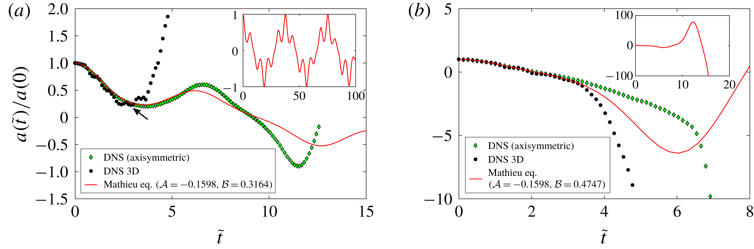
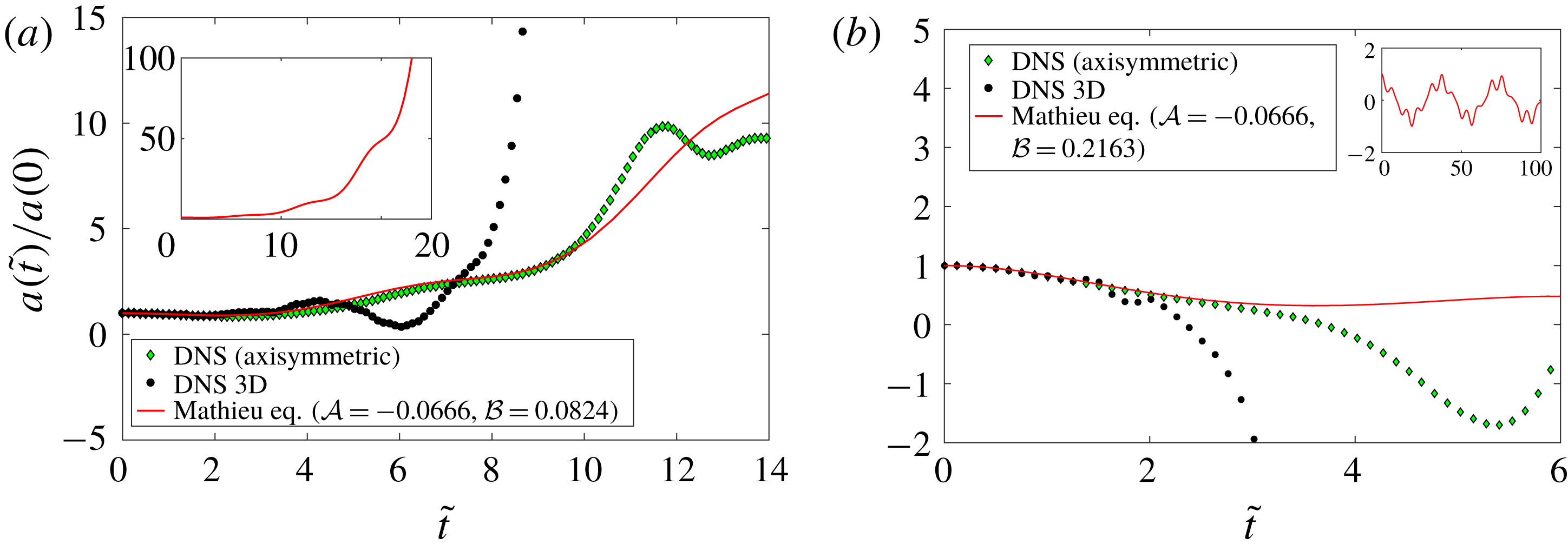
For small-amplitude perturbations, our linearised analytical predictions show excellent agreement with DNS in the stable and unstable regimes. Linear theory predicts that axisymmetric Fourier modes which are RP unstable in the absence of forcing are stabilised through forcing. Comparison of DNS with analytical predictions show that such stabilisation is achieved at early times. However, due to nonlinearity, higher modes are produced, some of which are unstable in the presence of forcing and which eventually destabilise the filament. For axisymmetric initial perturbations in the unstable regime and for sufficiently forcing amplitude, we find novel radially expanding sheet-like structures emanating from the cylindrical filament. Analogous structures also arise in the case of non-axisymmetric initial perturbations. These structures are strongly affected by nonlinearity and consequently their temporal evolution cannot be described by the Mathieu equation. In certain cases, these radially expanding structures are found to suffer further instabilities, leading to fragmentation and droplet generation. DNS results from parametric studies conducted in a space of five non-dimensional parameters are reported and comparisons of these with linearised predictions are provided. The paper is organised as follows: we begin with a derivation of the generalised Mathieu equation in § 2. This equation is applied to a cylindrical coordinate system in § 3 to study parametrically forced capillary oscillations on a cylindrical fluid filament, in the linearised limit. The simulation geometry is discussed in § 4. DNS results are analysed in § 5, where comparisons with analytical predictions are discussed, stabilisation of RP modes is examined and parametric studies are reported. We conclude with a discussion of further extension to the theory and scope of future work.
2 Generalised Mathieu equation
In this section we study the linear stability of an interface separating two inviscid, immiscible, quiescent fluids which are subjected to a time-periodic body force. The motivation for doing this is to generalise Faraday waves (seen, for example, when a partially filled rectangular container is vibrated vertically Benjamin & Ursell (Reference Benjamin and Ursell1954)) to non-Cartesian geometries (spherical and cylindrical) using an approach which unifies the three geometries. For Faraday waves in Cartesian geometry, in the frame of reference attached to the vibrated container, the effective acceleration due to gravity becomes time-periodic, acting perpendicular to the unperturbed interface (Benjamin & Ursell Reference Benjamin and Ursell1954). In the derivation that follows, this feature is generalised to a arbitrary orthogonal coordinate system where a time-periodic body force is imposed on both the fluids, acting in a direction normal to the unperturbed interface. The unperturbed interface (also called base state) is assumed to have a (constant) curvature (zero in the Cartesian case). To assist physical intuition, we provide a parallel derivation in § 1 in online supplementary material 1 (available at https://doi.org/10.1017/jfm.2018.657) which follows the generalised derivation provided here closely, but applies to the specific case of parametric oscillations on a cylindrical fluid filament.
Figure 1 shows part of the interface in the base state (in dark grey) separating two immiscible, quiescent fluids of density
 $\unicode[STIX]{x1D70C}^{{\mathcal{I}}}$
(superscripts
$\unicode[STIX]{x1D70C}^{{\mathcal{I}}}$
(superscripts
 ${\mathcal{I}}$
for inner fluid and
${\mathcal{I}}$
for inner fluid and
 $O$
for outer fluid) and
$O$
for outer fluid) and
 $\unicode[STIX]{x1D70C}^{O}$
with surface tension coefficient
$\unicode[STIX]{x1D70C}^{O}$
with surface tension coefficient
 $T$
. In the base state the interface is assumed to have a (constant) radius of curvature
$T$
. In the base state the interface is assumed to have a (constant) radius of curvature
 ${\mathcal{R}}$
(sum of the principal curvatures Bush (Reference Bush2013)). A local coordinate system is set up with two directions (locally) tangential to the base state interface indicated by
${\mathcal{R}}$
(sum of the principal curvatures Bush (Reference Bush2013)). A local coordinate system is set up with two directions (locally) tangential to the base state interface indicated by
 $(x_{\Vert }^{(1)},x_{\Vert }^{(2)})$
and a normal/vertical coordinate given by
$(x_{\Vert }^{(1)},x_{\Vert }^{(2)})$
and a normal/vertical coordinate given by
 $x_{\bot }$
(see figure 1). Both the fluids are subjected to a time-periodic body force
$x_{\bot }$
(see figure 1). Both the fluids are subjected to a time-periodic body force
 $G$
acting along the
$G$
acting along the
 $x_{\bot }$
direction, with
$x_{\bot }$
direction, with
 $G(x_{\bot },t)$
being a function only of the normal coordinate
$G(x_{\bot },t)$
being a function only of the normal coordinate
 $x_{\bot }$
and time
$x_{\bot }$
and time
 $t$
(analogous to gravitational force which varies only with the vertical coordinate
$t$
(analogous to gravitational force which varies only with the vertical coordinate
 $z$
). It is assumed that the Laplace equation admits variable separable solutions in this curvilinear coordinate system with generalised coordinates
$z$
). It is assumed that the Laplace equation admits variable separable solutions in this curvilinear coordinate system with generalised coordinates
 $\boldsymbol{x}\equiv (x_{\Vert }^{(1)},x_{\Vert }^{(2)},x_{\bot })\equiv (\boldsymbol{x}_{\Vert },x_{\bot })$
.
$\boldsymbol{x}\equiv (x_{\Vert }^{(1)},x_{\Vert }^{(2)},x_{\bot })\equiv (\boldsymbol{x}_{\Vert },x_{\bot })$
.
In this coordinate system, the equation for the interface in the base state is given by
 $x_{\bot }=\text{const.}\equiv x_{\bot }^{0}$
(see supplementary material 1 for specific examples for the choice of
$x_{\bot }=\text{const.}\equiv x_{\bot }^{0}$
(see supplementary material 1 for specific examples for the choice of
 $x_{\bot }^{0}$
). As the fluid velocity in the base state is zero (quiescent fluids), the base state pressure (
$x_{\bot }^{0}$
). As the fluid velocity in the base state is zero (quiescent fluids), the base state pressure (
 $P_{b}$
, subscript
$P_{b}$
, subscript
 $b$
for base state) in both the fluids satisfies the normal component of the inviscid momentum equations with the time-periodic body force
$b$
for base state) in both the fluids satisfies the normal component of the inviscid momentum equations with the time-periodic body force
 $G(x_{\bot },t)$
,
$G(x_{\bot },t)$
,
 $$\begin{eqnarray}\displaystyle -\frac{\unicode[STIX]{x2202}P_{b}^{{\mathcal{I}}}}{\unicode[STIX]{x2202}x_{\bot }}+\unicode[STIX]{x1D70C}^{{\mathcal{I}}}G(x_{\bot },t)=0,\quad -\frac{\unicode[STIX]{x2202}P_{b}^{O}}{\unicode[STIX]{x2202}x_{\bot }}+\unicode[STIX]{x1D70C}^{O}G(x_{\bot },t)=0. & & \displaystyle\end{eqnarray}$$
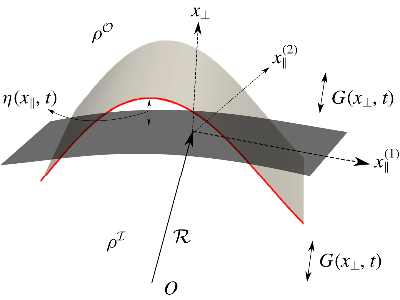
Figure 1. The base state is depicted as a dark grey surface while the perturbed interface is a light grey surface. The difference between the two is
 $\unicode[STIX]{x1D702}(x_{\Vert }^{(1)},x_{\Vert }^{(2)},t)$
.
$\unicode[STIX]{x1D702}(x_{\Vert }^{(1)},x_{\Vert }^{(2)},t)$
.
Integrating equations (2.1) in
 $x_{\bot }$
(one of the integration limits is taken to be
$x_{\bot }$
(one of the integration limits is taken to be
 $x_{\bot }^{0}$
), we obtain expressions for pressure in the base state,
$x_{\bot }^{0}$
), we obtain expressions for pressure in the base state,
 $$\begin{eqnarray}\displaystyle & \displaystyle P_{b}^{{\mathcal{I}}}(x_{\bot },t)=P_{b}^{{\mathcal{I}}}(x_{\bot }^{0},t)-\unicode[STIX]{x1D70C}^{{\mathcal{I}}}\int _{x_{\bot }}^{x_{\bot }^{0}}G(x^{\prime },t)\,\text{d}x^{\prime }, & \displaystyle\end{eqnarray}$$
 $$\begin{eqnarray}\displaystyle & \displaystyle P_{b}^{O}(x_{\bot },t)=P_{b}^{O}(x_{\bot }^{0},t)+\unicode[STIX]{x1D70C}^{O}\int _{x_{\bot }^{0}}^{x_{\bot }}G(x^{\prime },t)\,\text{d}x^{\prime }. & \displaystyle\end{eqnarray}$$
 $T$
and base state radius of curvature
$T$
and base state radius of curvature
 ${\mathcal{R}}$
(const.), the pressure-jump boundary condition at the interface is
${\mathcal{R}}$
(const.), the pressure-jump boundary condition at the interface is
 $P_{b}^{{\mathcal{I}}}(x_{\bot }^{0},t)-P_{b}^{O}(x_{\bot }^{0},t)=T/{\mathcal{R}}$
. We study the (linear) stability of the aforementioned time-periodic base state by imposing an interfacial perturbation. Using standard hydrodynamic stability techniques (Drazin Reference Drazin2002), all flow field variables (indicated with a tilde) are written as base (subscript
$P_{b}^{{\mathcal{I}}}(x_{\bot }^{0},t)-P_{b}^{O}(x_{\bot }^{0},t)=T/{\mathcal{R}}$
. We study the (linear) stability of the aforementioned time-periodic base state by imposing an interfacial perturbation. Using standard hydrodynamic stability techniques (Drazin Reference Drazin2002), all flow field variables (indicated with a tilde) are written as base (subscript
 $b$
) variable plus perturbation with subsequent linearisation in the perturbation variables. Assuming irrotational flow (i.e. zero vorticity) allows us to use the velocity potential
$b$
) variable plus perturbation with subsequent linearisation in the perturbation variables. Assuming irrotational flow (i.e. zero vorticity) allows us to use the velocity potential
 $\tilde{\unicode[STIX]{x1D719}}(\boldsymbol{x},t)$
. Expressing this and pressure
$\tilde{\unicode[STIX]{x1D719}}(\boldsymbol{x},t)$
. Expressing this and pressure
 $\tilde{p}(\boldsymbol{x},t)$
in the inner fluid as a sum of base and perturbation,
$\tilde{p}(\boldsymbol{x},t)$
in the inner fluid as a sum of base and perturbation,  $$\begin{eqnarray}\displaystyle \tilde{\unicode[STIX]{x1D719}}^{{\mathcal{I}}}(\boldsymbol{x},t)=0+\unicode[STIX]{x1D719}^{{\mathcal{I}}}(\boldsymbol{x},t),\quad \tilde{p}^{{\mathcal{I}}}(\boldsymbol{x},t)=P_{b}^{{\mathcal{I}}}(x_{\bot },t)+p^{{\mathcal{I}}}(\boldsymbol{x},t), & & \displaystyle\end{eqnarray}$$
with similar decompositions for the outer fluid.
 $\unicode[STIX]{x1D719}^{{\mathcal{I}}}$
and
$\unicode[STIX]{x1D719}^{{\mathcal{I}}}$
and
 $p^{{\mathcal{I}}}$
are the perturbation potential and pressure fields, respectively, generated in the inner fluid due to interfacial perturbation imposed at
$p^{{\mathcal{I}}}$
are the perturbation potential and pressure fields, respectively, generated in the inner fluid due to interfacial perturbation imposed at
 $t=0$
. The perturbation velocity potential
$t=0$
. The perturbation velocity potential
 $\unicode[STIX]{x1D719}$
satisfies the Laplace equation in both fluids (Debnath Reference Debnath1994),
$\unicode[STIX]{x1D719}$
satisfies the Laplace equation in both fluids (Debnath Reference Debnath1994),
 $$\begin{eqnarray}\displaystyle \unicode[STIX]{x1D6FB}^{2}\unicode[STIX]{x1D719}^{{\mathcal{I}}}(\boldsymbol{x},t)=0,\quad \unicode[STIX]{x1D6FB}^{2}\unicode[STIX]{x1D719}^{O}(\boldsymbol{x},t)=0. & & \displaystyle\end{eqnarray}$$
As shown in figure 1, the difference between the base state and perturbed interface is denoted by
 $\unicode[STIX]{x1D702}(\boldsymbol{x}_{\Vert },t)$
. The linearised kinematic boundary condition is (Debnath (Reference Debnath1994), equation (1.4.6))
$\unicode[STIX]{x1D702}(\boldsymbol{x}_{\Vert },t)$
. The linearised kinematic boundary condition is (Debnath (Reference Debnath1994), equation (1.4.6))
 $$\begin{eqnarray}\displaystyle \frac{\unicode[STIX]{x2202}\unicode[STIX]{x1D702}}{\unicode[STIX]{x2202}t}=\left(\unicode[STIX]{x1D735}\unicode[STIX]{x1D719}^{{\mathcal{I}}}\boldsymbol{\cdot }\hat{\boldsymbol{x}}_{\bot }\right)_{x_{\bot }=x_{\bot }^{0}}=\left(\unicode[STIX]{x1D735}\unicode[STIX]{x1D719}^{O}\boldsymbol{\cdot }\hat{\boldsymbol{x}}_{\bot }\right)_{x_{\bot }=x_{\bot }^{0}}, & & \displaystyle\end{eqnarray}$$
where
 $\hat{\boldsymbol{x}}_{\bot }$
is the unit normal to the unperturbed interface. The interfacial perturbation is chosen to be a standing wave, implying that the spatial and temporal parts are separable (see Prosperetti (Reference Prosperetti1976), Farsoiya et al. (Reference Farsoiya, Mayya and Dasgupta2017) for similar forms in other coordinate systems)
$\hat{\boldsymbol{x}}_{\bot }$
is the unit normal to the unperturbed interface. The interfacial perturbation is chosen to be a standing wave, implying that the spatial and temporal parts are separable (see Prosperetti (Reference Prosperetti1976), Farsoiya et al. (Reference Farsoiya, Mayya and Dasgupta2017) for similar forms in other coordinate systems)
 $$\begin{eqnarray}\displaystyle \unicode[STIX]{x1D702}(\boldsymbol{x}_{\Vert },t)=a(t)F(\boldsymbol{x}_{\Vert }), & & \displaystyle\end{eqnarray}$$
 $$\begin{eqnarray}\displaystyle \unicode[STIX]{x1D719}^{{\mathcal{I}}}(\boldsymbol{x}_{\Vert },x_{\bot },t)=F(\boldsymbol{x}_{\Vert })L^{{\mathcal{I}}}(x_{\bot }){\dot{a}}(t),\quad \unicode[STIX]{x1D719}^{O}(\boldsymbol{x},t)=F(\boldsymbol{x}_{\Vert })L^{O}(x_{\bot }){\dot{a}}(t). & & \displaystyle\end{eqnarray}$$
In (2.7), we have utilised the variable separability (of solutions to the Laplace equation) assumption, to express the velocity potential
 $\unicode[STIX]{x1D719}$
as a separable function of the coordinates
$\unicode[STIX]{x1D719}$
as a separable function of the coordinates
 $\boldsymbol{x}_{\Vert }=(x_{\Vert }^{(1)},x_{\Vert }^{(2)})$
and
$\boldsymbol{x}_{\Vert }=(x_{\Vert }^{(1)},x_{\Vert }^{(2)})$
and
 $x_{\bot }$
, with
$x_{\bot }$
, with
 $F$
,
$F$
,
 $L$
and
$L$
and
 $a(t)$
being as yet unknown functions of their argument and the dot over
$a(t)$
being as yet unknown functions of their argument and the dot over
 $a(t)$
indicating differentiation. The dependence of (2.7) on
$a(t)$
indicating differentiation. The dependence of (2.7) on
 ${\dot{a}}(t)$
ensures that the first equality in (2.5) is automatically satisfied. Our analysis is linearised, retaining terms up to
${\dot{a}}(t)$
ensures that the first equality in (2.5) is automatically satisfied. Our analysis is linearised, retaining terms up to
 $O(a(0))$
and we aim to obtain the equation governing
$O(a(0))$
and we aim to obtain the equation governing
 $a(t)$
, whose solution determines the stability of the time-periodic base state. In orthogonal curvilinear coordinates the Laplacian can be written as a sum of a horizontal (
$a(t)$
, whose solution determines the stability of the time-periodic base state. In orthogonal curvilinear coordinates the Laplacian can be written as a sum of a horizontal (
 $\unicode[STIX]{x1D6FB}_{\Vert }^{2}$
) and a vertical operator
$\unicode[STIX]{x1D6FB}_{\Vert }^{2}$
) and a vertical operator
 $\unicode[STIX]{x1D6FB}_{\bot }^{2}$
(see § 3 as well as supplementary material 1 for examples),
$\unicode[STIX]{x1D6FB}_{\bot }^{2}$
(see § 3 as well as supplementary material 1 for examples),
 $$\begin{eqnarray}\displaystyle \unicode[STIX]{x1D6FB}^{2}=\unicode[STIX]{x1D6FB}_{\Vert }^{2}+\unicode[STIX]{x1D6FB}_{\bot }^{2}. & & \displaystyle\end{eqnarray}$$
By definition, the horizontal (or vertical) part of the Laplacian contains derivatives with respect to the horizontal (or vertical) coordinates only. The function
 $F(\boldsymbol{x}_{\Vert })$
in (2.7) is chosen such that the horizontal part of the Laplacian operator
$F(\boldsymbol{x}_{\Vert })$
in (2.7) is chosen such that the horizontal part of the Laplacian operator
 $\unicode[STIX]{x1D6FB}_{\Vert }^{2}$
satisfies the eigenvalue relation
$\unicode[STIX]{x1D6FB}_{\Vert }^{2}$
satisfies the eigenvalue relation
 $$\begin{eqnarray}\displaystyle \unicode[STIX]{x1D6FB}_{\Vert }^{2}F(\boldsymbol{x}_{\Vert })=\unicode[STIX]{x1D706}(x_{\bot })F(\boldsymbol{x}_{\Vert }), & & \displaystyle\end{eqnarray}$$
where
 $\unicode[STIX]{x1D706}(x_{\bot })$
is the eigenvalue of
$\unicode[STIX]{x1D706}(x_{\bot })$
is the eigenvalue of
 $\unicode[STIX]{x1D6FB}_{\Vert }^{2}$
. Note that in Cartesian coordinates,
$\unicode[STIX]{x1D6FB}_{\Vert }^{2}$
. Note that in Cartesian coordinates,
 $\unicode[STIX]{x1D706}$
will be a constant. However, in curvilinear coordinate systems (such as cylindrical or spherical), the horizontal part of the Laplacian, i.e.
$\unicode[STIX]{x1D706}$
will be a constant. However, in curvilinear coordinate systems (such as cylindrical or spherical), the horizontal part of the Laplacian, i.e.
 $\unicode[STIX]{x1D6FB}_{\Vert }^{2}$
, may contain the vertical coordinate
$\unicode[STIX]{x1D6FB}_{\Vert }^{2}$
, may contain the vertical coordinate
 $x_{\bot }$
(but not derivatives with respect to
$x_{\bot }$
(but not derivatives with respect to
 $x_{\bot }$
), and consequently the eigenvalue
$x_{\bot }$
), and consequently the eigenvalue
 $\unicode[STIX]{x1D706}(x_{\bot })$
can be a function of the vertical coordinate
$\unicode[STIX]{x1D706}(x_{\bot })$
can be a function of the vertical coordinate
 $x_{\bot }$
. Substituting expressions (2.7) into the Laplace equations (2.4) for inner and outer fluids and using decomposition (2.8) and (2.9), we obtain
$x_{\bot }$
. Substituting expressions (2.7) into the Laplace equations (2.4) for inner and outer fluids and using decomposition (2.8) and (2.9), we obtain
 $$\begin{eqnarray}\displaystyle & \displaystyle \unicode[STIX]{x1D706}(x_{\bot })F(\boldsymbol{x}_{\Vert })L^{{\mathcal{I}}}(x_{\bot }){\dot{a}}(t)+F(\boldsymbol{x}_{\Vert }){\dot{a}}(t)\unicode[STIX]{x1D6FB}_{\bot }^{2}L^{{\mathcal{I}}}=0 & \displaystyle\end{eqnarray}$$
 $$\begin{eqnarray}\displaystyle & \displaystyle \text{and}\quad \unicode[STIX]{x1D706}(x_{\bot })F(\boldsymbol{x}_{\Vert })L^{O}(x_{\bot }){\dot{a}}(t)+F(\boldsymbol{x}_{\Vert }){\dot{a}}(t)\unicode[STIX]{x1D6FB}_{\bot }^{2}L^{O}=0, & \displaystyle\end{eqnarray}$$
which can be rewritten as
 $$\begin{eqnarray}\displaystyle \unicode[STIX]{x1D6FB}_{\bot }^{2}L^{{\mathcal{I}}}+\unicode[STIX]{x1D706}(x_{\bot })L^{{\mathcal{I}}}(x_{\bot })=0,\quad \unicode[STIX]{x1D6FB}_{\bot }^{2}L^{O}+\unicode[STIX]{x1D706}(x_{\bot })L^{O}(x_{\bot })=0. & & \displaystyle\end{eqnarray}$$
Equations (2.12) are (in general) linear, variable coefficient second-order equations and general closed form solutions are not known. The general solution for each equation can be written as a linear combination of two linearly independent solutions, requiring two boundary conditions. One of these is the requirement that at
 $x_{\bot }=\pm \infty$
or 0,
$x_{\bot }=\pm \infty$
or 0,
 $L(x_{\bot })$
remains finite, i.e.
$L(x_{\bot })$
remains finite, i.e.
 $$\begin{eqnarray}\displaystyle L^{{\mathcal{I}}}(x_{\bot }\rightarrow 0\;\text{or}\;-\infty )\rightarrow \text{finite}\quad \text{and}\quad L^{O}(x_{\bot }\rightarrow \infty )\rightarrow \text{finite}. & & \displaystyle\end{eqnarray}$$
The second boundary condition is obtained from (2.5). The gradient of
 $\unicode[STIX]{x1D719}$
in generalised coordinates can be written as (Weisstein Reference Weisstein2017a
)
$\unicode[STIX]{x1D719}$
in generalised coordinates can be written as (Weisstein Reference Weisstein2017a
)
 $$\begin{eqnarray}\displaystyle \unicode[STIX]{x1D735}\unicode[STIX]{x1D719}=\mathop{\sum }_{i=1}^{2}\frac{1}{h_{i}}\frac{\unicode[STIX]{x2202}\unicode[STIX]{x1D719}}{\unicode[STIX]{x2202}x_{\Vert }^{(i)}}\hat{\boldsymbol{x}}_{\Vert }^{(i)}+\frac{1}{h_{3}}\frac{\unicode[STIX]{x2202}\unicode[STIX]{x1D719}}{\unicode[STIX]{x2202}x_{\bot }}\hat{\boldsymbol{x}}_{\bot }, & & \displaystyle\end{eqnarray}$$
where
 $h_{i}$
are the scale factors (Weisstein Reference Weisstein2017e
) and
$h_{i}$
are the scale factors (Weisstein Reference Weisstein2017e
) and
 $\hat{\boldsymbol{x}}_{\Vert }^{(i)}$
(
$\hat{\boldsymbol{x}}_{\Vert }^{(i)}$
(
 $i=1,2$
) and
$i=1,2$
) and
 $\hat{\boldsymbol{x}}_{\bot }$
are unit vectors along the tangential and normal directions to the unperturbed interface (see figure 1). Substituting expression (2.14) in (2.5) we obtain
$\hat{\boldsymbol{x}}_{\bot }$
are unit vectors along the tangential and normal directions to the unperturbed interface (see figure 1). Substituting expression (2.14) in (2.5) we obtain
 $$\begin{eqnarray}\displaystyle \left(\frac{\text{d}L^{{\mathcal{I}}}}{\text{d}x_{\bot }}\right)_{x_{\bot }=x_{\bot }^{0}}=\left(\frac{\text{d}L^{O}}{\text{d}x_{\bot }}\right)_{x_{\bot }=x_{\bot }^{0}}=1. & & \displaystyle\end{eqnarray}$$
This last equality in (2.15) uses
 $h_{3}=1$
, as it is the scale factor of the vertical coordinate
$h_{3}=1$
, as it is the scale factor of the vertical coordinate
 $x_{\bot }$
, which always has the units of distance. Equation (2.15) is the second boundary condition for determining the unknown constant of integration in the expression for
$x_{\bot }$
, which always has the units of distance. Equation (2.15) is the second boundary condition for determining the unknown constant of integration in the expression for
 $L(x_{\bot })$
. In the presence of an interfacial perturbation, the difference of total pressure (base
$L(x_{\bot })$
. In the presence of an interfacial perturbation, the difference of total pressure (base
 $+$
perturbation) on either side of the interface equals the surface tension coefficient
$+$
perturbation) on either side of the interface equals the surface tension coefficient
 $T$
times the surface divergence of the unit normal at the perturbed interface (Prosperetti Reference Prosperetti1976, Reference Prosperetti1981),
$T$
times the surface divergence of the unit normal at the perturbed interface (Prosperetti Reference Prosperetti1976, Reference Prosperetti1981),
 $$\begin{eqnarray}\displaystyle & & \displaystyle P_{b}^{{\mathcal{I}}}(x_{\bot }^{0}+\unicode[STIX]{x1D702},t)+p^{{\mathcal{I}}}(\boldsymbol{x}_{\Vert },x_{\bot }=x_{\bot }^{0},t)\nonumber\\ \displaystyle & & \displaystyle \qquad -\,P_{b}^{O}(x_{\bot }^{0}+\unicode[STIX]{x1D702},t)-p^{O}(\boldsymbol{x}_{\Vert },x_{\bot }=x_{\bot }^{0},t)=T\left(\unicode[STIX]{x1D735}\boldsymbol{\cdot }\boldsymbol{q}\right)_{x_{\bot }=x_{\bot }^{0}+\unicode[STIX]{x1D702}},\end{eqnarray}$$
where
 $\boldsymbol{q}$
is the unit normal to the perturbed interface and the perturbation pressure
$\boldsymbol{q}$
is the unit normal to the perturbed interface and the perturbation pressure
 $p$
is evaluated at the unperturbed interface
$p$
is evaluated at the unperturbed interface
 $x_{\bot }^{0}$
in order to retain terms only up to
$x_{\bot }^{0}$
in order to retain terms only up to
 $O(a(0))$
. In order to compute curvature at the perturbed interface we define (Bush Reference Bush2013)
$O(a(0))$
. In order to compute curvature at the perturbed interface we define (Bush Reference Bush2013)
 $$\begin{eqnarray}\displaystyle Q(\boldsymbol{x}_{\Vert },x_{\bot },t)\equiv x_{\bot }-x_{\bot }^{0}-\unicode[STIX]{x1D702}(\boldsymbol{x}_{\Vert },t)=x_{\bot }-x_{\bot }^{0}-a(t)F(\boldsymbol{x}_{\Vert }). & & \displaystyle\end{eqnarray}$$
At a linear approximation, the divergence of
 $\boldsymbol{q}$
equals the Laplacian of
$\boldsymbol{q}$
equals the Laplacian of
 $Q$
(see equation 5.37 in Bush (Reference Bush2013)). Thus, from (2.17), expressions (2.6), decomposition (2.8) and (2.9) up to linear order in
$Q$
(see equation 5.37 in Bush (Reference Bush2013)). Thus, from (2.17), expressions (2.6), decomposition (2.8) and (2.9) up to linear order in
 $a(0)$
we have
$a(0)$
we have
 $$\begin{eqnarray}\displaystyle \left(\unicode[STIX]{x1D735}\boldsymbol{\cdot }\boldsymbol{q}\right)_{x_{\bot }=x_{\bot }^{0}+\unicode[STIX]{x1D702}} & {\approx} & \displaystyle \left(\unicode[STIX]{x1D6FB}^{2}Q\right)_{x_{\bot }=x_{\bot }^{0}+\unicode[STIX]{x1D702}}=\unicode[STIX]{x1D712}(x_{\bot }^{0}+\unicode[STIX]{x1D702})-a(t)\unicode[STIX]{x1D6FB}_{\Vert }^{2}F(\boldsymbol{x}_{\Vert })\nonumber\\ \displaystyle & {\approx} & \displaystyle \unicode[STIX]{x1D712}(x_{\bot }^{0})+\left(\frac{\text{d}\unicode[STIX]{x1D712}}{\text{d}x_{\bot }}\right)_{x_{\bot }^{0}}\unicode[STIX]{x1D702}(\boldsymbol{x}_{\Vert },t)-a(t)\unicode[STIX]{x1D706}(x_{\bot }^{0})F(\boldsymbol{x}_{\Vert }),\end{eqnarray}$$
where
 $\unicode[STIX]{x1D712}(x_{\bot })\equiv \unicode[STIX]{x1D6FB}_{\bot }^{2}(x_{\bot })$
and
$\unicode[STIX]{x1D712}(x_{\bot })\equiv \unicode[STIX]{x1D6FB}_{\bot }^{2}(x_{\bot })$
and
 $\unicode[STIX]{x1D712}(x_{\bot }^{0})$
is an
$\unicode[STIX]{x1D712}(x_{\bot }^{0})$
is an
 $O(1)$
term arising from base state curvature (zero in the rectangular Cartesian case) satisfying by definition
$O(1)$
term arising from base state curvature (zero in the rectangular Cartesian case) satisfying by definition
 $(1/{\mathcal{R}})=\unicode[STIX]{x1D712}(x_{\bot }^{0})$
(see figure 1). In writing the second line after (2.18), we have Taylor expanded
$(1/{\mathcal{R}})=\unicode[STIX]{x1D712}(x_{\bot }^{0})$
(see figure 1). In writing the second line after (2.18), we have Taylor expanded
 $\unicode[STIX]{x1D712}(x_{\bot })$
about
$\unicode[STIX]{x1D712}(x_{\bot })$
about
 $x_{\bot }^{0}$
, retaining terms up to
$x_{\bot }^{0}$
, retaining terms up to
 $O(a(0))$
through
$O(a(0))$
through
 $\unicode[STIX]{x1D702}$
. An expression for the difference of base pressures on the left-hand side of (2.16) can be obtained using (2.2). After some simple algebraic manipulations, this is
$\unicode[STIX]{x1D702}$
. An expression for the difference of base pressures on the left-hand side of (2.16) can be obtained using (2.2). After some simple algebraic manipulations, this is
 $$\begin{eqnarray}\displaystyle P_{b}^{{\mathcal{I}}}(x_{\bot }^{0}+\unicode[STIX]{x1D702},t)-P_{b}^{O}(x_{\bot }^{0}+\unicode[STIX]{x1D702},t)=\frac{T}{{\mathcal{R}}}-\left(\unicode[STIX]{x1D70C}^{{\mathcal{I}}}-\unicode[STIX]{x1D70C}^{O}\right)\int _{x_{\bot }^{0}+\unicode[STIX]{x1D702}}^{x_{\bot }^{0}}G(x^{\prime },t)\,\text{d}x^{\prime }, & & \displaystyle\end{eqnarray}$$
where we have used the base state pressure-jump condition to replace
 $P_{b}^{{\mathcal{I}}}(x_{\bot }^{0},t)-P_{b}^{O}(x_{\bot }^{0},t)$
with
$P_{b}^{{\mathcal{I}}}(x_{\bot }^{0},t)-P_{b}^{O}(x_{\bot }^{0},t)$
with
 $T/{\mathcal{R}}$
(see below (2.2)). Defining
$T/{\mathcal{R}}$
(see below (2.2)). Defining
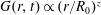
 $G(x_{\bot },t)\equiv \unicode[STIX]{x2202}\unicode[STIX]{x1D6F9}/\unicode[STIX]{x2202}x_{\bot }$
and using Taylor series expansion, we find an approximation to the integral in (2.19) as
$G(x_{\bot },t)\equiv \unicode[STIX]{x2202}\unicode[STIX]{x1D6F9}/\unicode[STIX]{x2202}x_{\bot }$
and using Taylor series expansion, we find an approximation to the integral in (2.19) as
 $$\begin{eqnarray}\displaystyle \int _{x_{\bot }^{0}+\unicode[STIX]{x1D702}}^{x_{\bot }^{0}}G(x^{\prime },t)\,\text{d}x^{\prime }=\unicode[STIX]{x1D6F9}(x_{\bot }^{0},t)-\unicode[STIX]{x1D6F9}(x_{\bot }^{0}+\unicode[STIX]{x1D702},t)\approx -G(x_{\bot }^{0},t)\unicode[STIX]{x1D702}(\boldsymbol{x}_{\Vert },t)+O(\unicode[STIX]{x1D702}^{2}). & & \displaystyle\end{eqnarray}$$
Using (2.16) with (2.18), (2.19), (2.20) (after cancelling out the base state contribution to pressure using
 $(1/{\mathcal{R}})=\unicode[STIX]{x1D712}(x_{\bot }^{0})$
, see text below (2.18)), we obtain
$(1/{\mathcal{R}})=\unicode[STIX]{x1D712}(x_{\bot }^{0})$
, see text below (2.18)), we obtain
 $$\begin{eqnarray}\displaystyle \left(\unicode[STIX]{x1D70C}^{{\mathcal{I}}}-\unicode[STIX]{x1D70C}^{O}\right)G(x_{\bot }^{0},t)\unicode[STIX]{x1D702}(\boldsymbol{x}_{\Vert },t)+\left(p^{{\mathcal{I}}}-p^{O}\right)_{x_{\bot }=x_{\bot }^{0}}=T\left[\left(\frac{\text{d}\unicode[STIX]{x1D712}}{\text{d}x_{\bot }}\right)_{x_{\bot }^{0}}-\unicode[STIX]{x1D706}(x_{\bot }^{0})\right]a(t)F(\boldsymbol{x}_{\Vert }) & & \displaystyle \nonumber\\ \displaystyle & & \displaystyle\end{eqnarray}$$
The (linearised) unsteady Bernoulli equation for the perturbation pressure at the linearised interface (Farsoiya et al. Reference Farsoiya, Mayya and Dasgupta2017) is
 $$\begin{eqnarray}\displaystyle \left(p^{{\mathcal{I}}}-p^{O}\right)_{x_{\bot }=x_{\bot }^{0}}=\left(\unicode[STIX]{x1D70C}^{O}\frac{\unicode[STIX]{x2202}\unicode[STIX]{x1D719}^{O}}{\unicode[STIX]{x2202}t}-\unicode[STIX]{x1D70C}^{{\mathcal{I}}}\frac{\unicode[STIX]{x2202}\unicode[STIX]{x1D719}^{{\mathcal{I}}}}{\unicode[STIX]{x2202}t}\right)_{x_{\bot }=x_{\bot }^{0}}. & & \displaystyle\end{eqnarray}$$
Substituting the expression for perturbation pressure
 $p$
from (2.22) in (2.21) and using (2.7), we obtain a Mathieu equation for
$p$
from (2.22) in (2.21) and using (2.7), we obtain a Mathieu equation for
 $a(t)$
of the form
$a(t)$
of the form
 $$\begin{eqnarray}\displaystyle \ddot{a}(t)+f(t)a(t)=0, & & \displaystyle\end{eqnarray}$$
with
 $$\begin{eqnarray}\displaystyle f(t)\equiv \left\{\frac{T\left({\displaystyle \frac{\text{d}\unicode[STIX]{x1D712}}{\text{d}x_{\bot }}}-\unicode[STIX]{x1D706}(x_{\bot })\right)-\left(\unicode[STIX]{x1D70C}^{{\mathcal{I}}}-\unicode[STIX]{x1D70C}^{O}\right)G(x_{\bot },t)}{\unicode[STIX]{x1D70C}^{{\mathcal{I}}}L^{{\mathcal{I}}}(x_{\bot })-\unicode[STIX]{x1D70C}^{O}L^{O}(x_{\bot })}\right\}_{x_{\bot }=x_{\bot }^{0}}. & & \displaystyle\end{eqnarray}$$
Equation (2.23) is the generalised equation governing Faraday waves on an interface. It can be applied to four base state geometries, as seen in figure 2, and governs Faraday waves in each (see derivations in supplementary material 1). For zero forcing,
 $G=0$
, it leads to the dispersion relation for free perturbations, as demonstrated in the next section for a capillary filament and for other classical, free oscillation problems (see accompanying supplementary material 1).
$G=0$
, it leads to the dispersion relation for free perturbations, as demonstrated in the next section for a capillary filament and for other classical, free oscillation problems (see accompanying supplementary material 1).
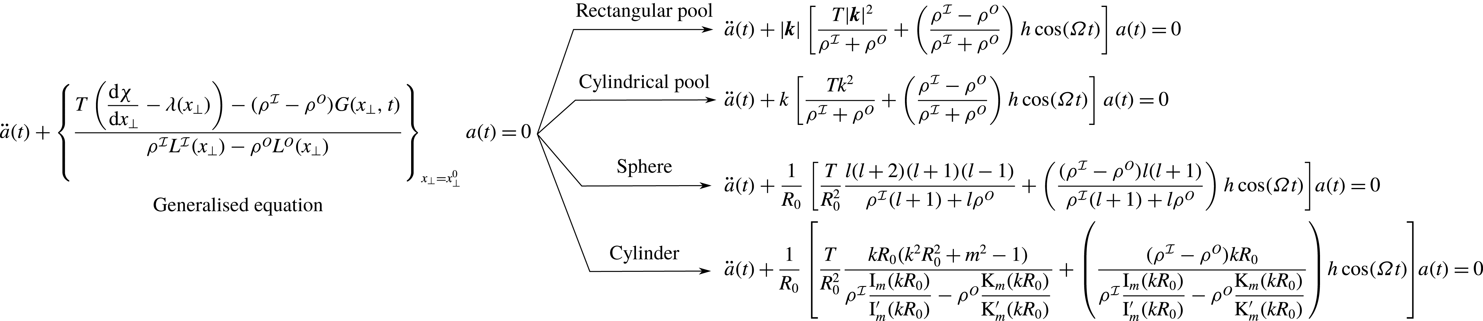
Figure 2. Applications of the generalised equation (2.23) to obtain the equation governing Faraday waves on various base state geometries. The Mathieu equation on horizontally unbounded rectangular and cylindrical pools was obtained by Benjamin & Ursell (Reference Benjamin and Ursell1954), on a spherical droplet by Adou & Tuckerman (Reference Adou and Tuckerman2016), and on a cylindrical filament in the present study. From top to bottom, the derivation of the first three cases from the generalised equation (2.23) are provided in supplementary material 1.

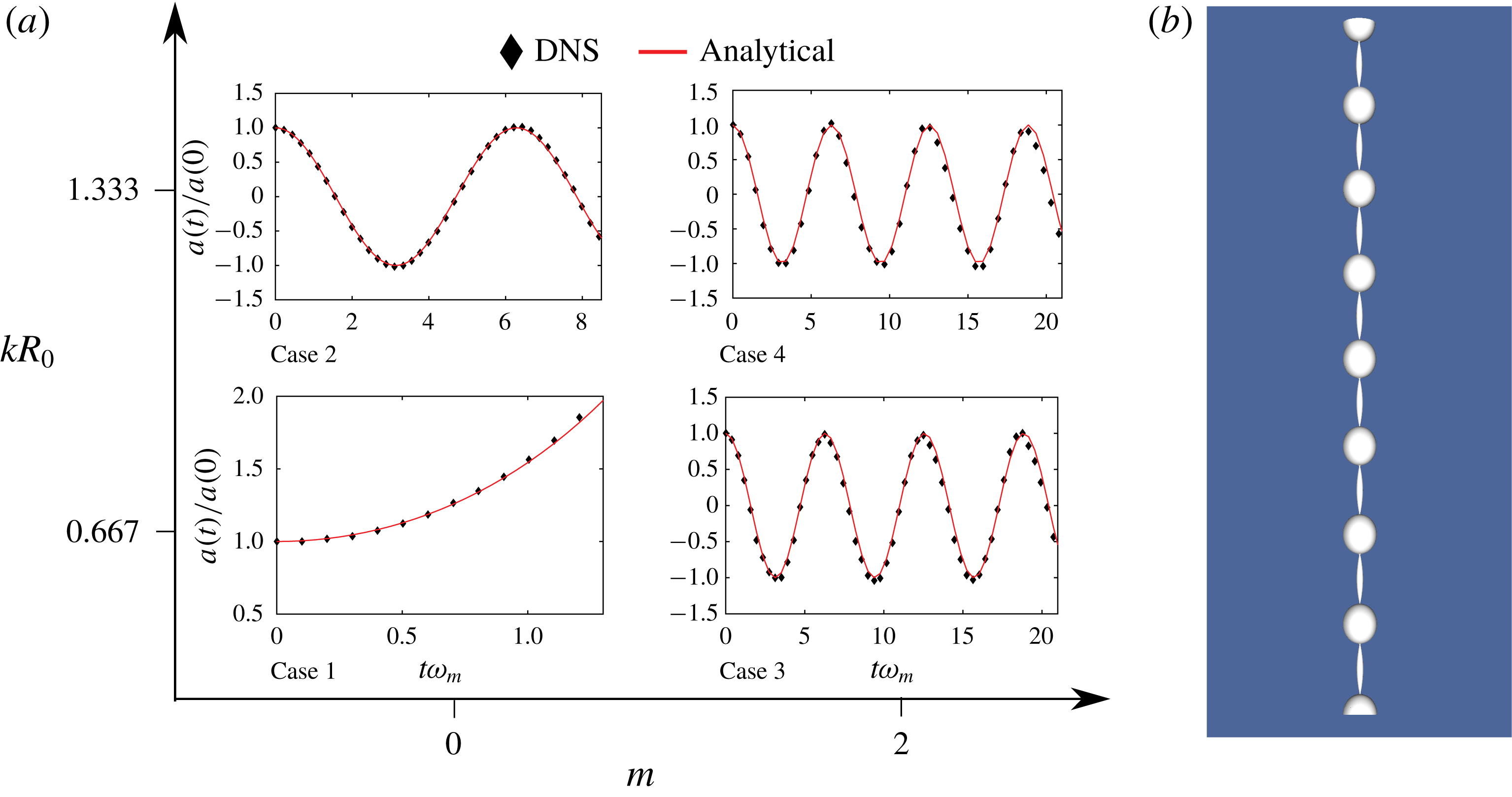
Figure 3. A capillary filament. In (b) the perturbed surface is in grey, the unperturbed surface is shown using lines. (a) Unperturbed interface. (b) Perturbed interface.
3 Perturbations of a cylindrical fluid filament
3.1 Free perturbations
We use expression (2.24) to obtain the dispersion relation of perturbations on a cylindrical interface between two inviscid fluids (Rayleigh 1879; Lamb Reference Lamb1932). The base state is a cylindrical capillary filament of radius
 $R_{0}$
separating two immiscible quiescent fluids of density
$R_{0}$
separating two immiscible quiescent fluids of density
 $\unicode[STIX]{x1D70C}^{{\mathcal{I}}}$
and
$\unicode[STIX]{x1D70C}^{{\mathcal{I}}}$
and
 $\unicode[STIX]{x1D70C}^{O}$
and surface tension
$\unicode[STIX]{x1D70C}^{O}$
and surface tension
 $T$
, as seen in figure 3. We impose perturbations of azimuthal wavenumber
$T$
, as seen in figure 3. We impose perturbations of azimuthal wavenumber
 $m$
and axial wavenumber
$m$
and axial wavenumber
 $k$
on the interface. The time-periodic body force
$k$
on the interface. The time-periodic body force
 $G$
is set to zero for free oscillations.
$G$
is set to zero for free oscillations.
For the cylindrical coordinate system used here, the coordinates tangential to the unperturbed cylinder are
 $x_{\Vert }^{(1)}=\unicode[STIX]{x1D703}$
,
$x_{\Vert }^{(1)}=\unicode[STIX]{x1D703}$
,
 $x_{\Vert }^{(2)}=z$
, the vertical coordinate
$x_{\Vert }^{(2)}=z$
, the vertical coordinate
 $x_{\bot }=r$
and the unperturbed cylinder has the equation
$x_{\bot }=r$
and the unperturbed cylinder has the equation
 $r=R_{0}=x_{\bot }^{0}$
, the radius of the cylindrical filament (see figure 3). The Laplacian operator in this coordinate system is given by Weisstein (Reference Weisstein2017d
)
$r=R_{0}=x_{\bot }^{0}$
, the radius of the cylindrical filament (see figure 3). The Laplacian operator in this coordinate system is given by Weisstein (Reference Weisstein2017d
)
 $$\begin{eqnarray}\displaystyle \unicode[STIX]{x1D6FB}^{2}=\unicode[STIX]{x1D6FB}_{\Vert }^{2}+\unicode[STIX]{x1D6FB}_{\bot }^{2}=\left(\frac{1}{r^{2}}\frac{\unicode[STIX]{x2202}^{2}}{\unicode[STIX]{x2202}\unicode[STIX]{x1D703}^{2}}+\frac{\unicode[STIX]{x2202}^{2}}{\unicode[STIX]{x2202}z^{2}}\right)+\frac{1}{r}\frac{\unicode[STIX]{x2202}}{\unicode[STIX]{x2202}r}\left(r\frac{\unicode[STIX]{x2202}}{\unicode[STIX]{x2202}r}\right). & & \displaystyle\end{eqnarray}$$
 $\unicode[STIX]{x1D6FB}_{\Vert }^{2}$
satisfies
$\unicode[STIX]{x1D6FB}_{\Vert }^{2}$
satisfies
 $$\begin{eqnarray}\displaystyle \left(\frac{1}{r^{2}}\frac{\unicode[STIX]{x2202}^{2}}{\unicode[STIX]{x2202}\unicode[STIX]{x1D703}^{2}}+\frac{\unicode[STIX]{x2202}^{2}}{\unicode[STIX]{x2202}z^{2}}\right)\cos (m\unicode[STIX]{x1D703})\cos (kz)=-\left(\frac{m^{2}}{r^{2}}+k^{2}\right)\cos (m\unicode[STIX]{x1D703})\cos (kz). & & \displaystyle\end{eqnarray}$$
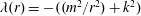
Hence for this problem the eigenvalue for
 $\unicode[STIX]{x1D6FB}_{\Vert }^{2}$
is
$\unicode[STIX]{x1D6FB}_{\Vert }^{2}$
is
 $\unicode[STIX]{x1D706}(r)=-((m^{2}/r^{2})+k^{2})$
and the equation governing
$\unicode[STIX]{x1D706}(r)=-((m^{2}/r^{2})+k^{2})$
and the equation governing
 $L(r)$
is (see (2.12))
$L(r)$
is (see (2.12))
 $$\begin{eqnarray}\displaystyle \frac{1}{r}\frac{\text{d}}{\text{d}r}\left(r\frac{\text{d}L^{{\mathcal{I}}}}{\text{d}r}\right)-\left(\frac{m^{2}}{r^{2}}+k^{2}\right)L^{{\mathcal{I}}}(r)=0,\quad \frac{1}{r}\frac{\text{d}}{\text{d}r}\left(r\frac{\text{d}L^{O}}{\text{d}r}\right)-\left(\frac{m^{2}}{r^{2}}+k^{2}\right)L^{O}(r)=0. & & \displaystyle \nonumber\\ \displaystyle & & \displaystyle\end{eqnarray}$$
The above equations have the solution (see expression (6.2.28) in Prosperetti (Reference Prosperetti2011))
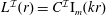 $L^{{\mathcal{I}}}(r)=C^{{\mathcal{I}}}\text{I}_{m}(kr)$
and
$L^{{\mathcal{I}}}(r)=C^{{\mathcal{I}}}\text{I}_{m}(kr)$
and
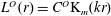 $L^{O}(r)=C^{O}\text{K}_{m}(kr)$
using boundedness at
$L^{O}(r)=C^{O}\text{K}_{m}(kr)$
using boundedness at
 $r=0$
and
$r=0$
and
 $r\rightarrow \infty$
respectively (i.e. generalised boundary conditions (2.17), Weisstein (Reference Weisstein2017b
,Reference Weisstein
c
)) where
$r\rightarrow \infty$
respectively (i.e. generalised boundary conditions (2.17), Weisstein (Reference Weisstein2017b
,Reference Weisstein
c
)) where
 $\text{I}_{m}(z)$
and
$\text{I}_{m}(z)$
and
 $\text{K}_{m}(z)$
are modified Bessel’s function. Using generalised boundary condition (2.15), we determine
$\text{K}_{m}(z)$
are modified Bessel’s function. Using generalised boundary condition (2.15), we determine
 $C^{{\mathcal{I}}}$
and
$C^{{\mathcal{I}}}$
and
 $C^{O}$
to obtain
$C^{O}$
to obtain
 $$\begin{eqnarray}\displaystyle L^{{\mathcal{I}}}(r)=\frac{\text{I}_{m}(kr)}{k\text{I}_{m}^{\prime }(kR_{0})}\quad \text{and}\quad L^{O}(r)=\frac{\text{K}_{m}(kr)}{k\text{K}_{m}^{\prime }(kR_{0})}, & & \displaystyle\end{eqnarray}$$
where
 $\text{I}_{m}^{\prime }(z)\equiv (\text{d}\text{I}_{m}/\text{d}z)$
etc. In this coordinate system (see text below (2.18))
$\text{I}_{m}^{\prime }(z)\equiv (\text{d}\text{I}_{m}/\text{d}z)$
etc. In this coordinate system (see text below (2.18))
 $\unicode[STIX]{x1D712}(r)\equiv (\unicode[STIX]{x1D6FB}_{\bot }^{2})r=(1/r)(\unicode[STIX]{x2202}/\unicode[STIX]{x2202}r)(r(\unicode[STIX]{x2202}/\unicode[STIX]{x2202}r))r=1/r$
and we obtain the value of
$\unicode[STIX]{x1D712}(r)\equiv (\unicode[STIX]{x1D6FB}_{\bot }^{2})r=(1/r)(\unicode[STIX]{x2202}/\unicode[STIX]{x2202}r)(r(\unicode[STIX]{x2202}/\unicode[STIX]{x2202}r))r=1/r$
and we obtain the value of
 $f(t)\equiv \unicode[STIX]{x1D714}_{m}^{2}$
(with
$f(t)\equiv \unicode[STIX]{x1D714}_{m}^{2}$
(with
 $G(r,t)=0$
) from expression (2.24) as
$G(r,t)=0$
) from expression (2.24) as
 $$\begin{eqnarray}\displaystyle \unicode[STIX]{x1D714}_{m}^{2}(k)=\frac{T}{R_{0}^{3}}\left[\frac{kR_{0}\left(k^{2}R_{0}^{2}+m^{2}-1\right)}{\unicode[STIX]{x1D70C}^{{\mathcal{I}}}{\displaystyle \frac{\text{I}_{m}(kR_{0})}{\text{I}_{m}^{\prime }(kR_{0})}}-\unicode[STIX]{x1D70C}^{O}{\displaystyle \frac{\text{K}_{m}(kR_{0})}{\text{K}_{m}^{\prime }(kR_{0})}}}\right]. & & \displaystyle\end{eqnarray}$$
Expression (3.5) is the dispersion relation governing linearised perturbations of an inviscid cylindrical filament immersed in another inviscid fluid. It generalises equation (12) in Meister & Scheele (Reference Meister and Scheele1967), who discuss the inviscid case of RP instability taking into account the density of both fluids for the case of axisymmetric perturbations (
 $m=0$
). For the case of free perturbations, the Mathieu equation (2.23) becomes the simple harmonic oscillator equation,
$m=0$
). For the case of free perturbations, the Mathieu equation (2.23) becomes the simple harmonic oscillator equation,
 $$\begin{eqnarray}\displaystyle \frac{\text{d}^{2}a}{\text{d}t^{2}}+\unicode[STIX]{x1D714}_{m}^{2}(k)a(t)=0. & & \displaystyle\end{eqnarray}$$
3.2 Parametrically forced standing waves
For studying parametric forced standing waves on the cylindrical filament (see figure 7
c for geometry of forcing), we set
 $G(r,t)=-h\cos (\unicode[STIX]{x1D6FA}t)(r/R_{0})$
as a linearly varying function of radial position
$G(r,t)=-h\cos (\unicode[STIX]{x1D6FA}t)(r/R_{0})$
as a linearly varying function of radial position
 $r$
and acting radially (see figure 7
c,d). We follow Adou & Tuckerman (Reference Adou and Tuckerman2016) in regularising the singularity (multivaluedness) on the axis of the filament
$r$
and acting radially (see figure 7
c,d). We follow Adou & Tuckerman (Reference Adou and Tuckerman2016) in regularising the singularity (multivaluedness) on the axis of the filament
 $r=0$
using a linear spatial variation of the body force, i.e.
$r=0$
using a linear spatial variation of the body force, i.e.
 $G(r,t)\propto r/R_{0}$
. Choosing a nonlinear variation of the form
$G(r,t)\propto r/R_{0}$
. Choosing a nonlinear variation of the form
 $G(r,t)\propto (r/R_{0})^{z}$
with
$G(r,t)\propto (r/R_{0})^{z}$
with
 $z=2\ldots$
does not alter our results qualitatively, since in a linearised description the coefficient of (3.7) is evaluated at
$z=2\ldots$
does not alter our results qualitatively, since in a linearised description the coefficient of (3.7) is evaluated at
 $r=R_{0}$
. The Mathieu equation (2.23) in the cylindrical geometry now becomes
$r=R_{0}$
. The Mathieu equation (2.23) in the cylindrical geometry now becomes
 $$\begin{eqnarray}\displaystyle \frac{\text{d}^{2}a}{\text{d}t^{2}}+\left[\unicode[STIX]{x1D714}_{m}^{2}(k)+\frac{\left(\unicode[STIX]{x1D70C}^{{\mathcal{I}}}-\unicode[STIX]{x1D70C}^{O}\right)hk\cos (\unicode[STIX]{x1D6FA}t)}{\unicode[STIX]{x1D70C}^{{\mathcal{I}}}{\displaystyle \frac{\text{I}_{m}(kR_{0})}{\text{I}_{m}^{\prime }(kR_{0})}}-\unicode[STIX]{x1D70C}^{O}{\displaystyle \frac{\text{K}_{m}(kR_{0})}{\text{K}_{m}^{\prime }(kR_{0})}}}\right]a(t)=0, & & \displaystyle\end{eqnarray}$$
where
 $\unicode[STIX]{x1D714}_{m}^{2}(k)$
is given by (3.5). Equation (3.7) can be rewritten compactly as (in the same notation as Bender & Orszag (Reference Bender and Orszag2010)),
$\unicode[STIX]{x1D714}_{m}^{2}(k)$
is given by (3.5). Equation (3.7) can be rewritten compactly as (in the same notation as Bender & Orszag (Reference Bender and Orszag2010)),
 $$\begin{eqnarray}\displaystyle \frac{\text{d}^{2}a}{\text{d}\tilde{t}^{2}}+\left({\mathcal{A}}+2{\mathcal{B}}\cos (\tilde{t})\right)a(\tilde{t})=0, & & \displaystyle\end{eqnarray}$$
where
 $\tilde{t}\equiv \unicode[STIX]{x1D6FA}t$
,
$\tilde{t}\equiv \unicode[STIX]{x1D6FA}t$
,
 $$\begin{eqnarray}\displaystyle {\mathcal{A}}=\left(\frac{\unicode[STIX]{x1D714}_{m}(k)}{\unicode[STIX]{x1D6FA}}\right)^{2}\quad \text{and}\quad {\mathcal{B}}\equiv \frac{h}{2\unicode[STIX]{x1D6FA}^{2}}\left[((\unicode[STIX]{x1D70C}^{{\mathcal{I}}}-\unicode[STIX]{x1D70C}^{O})k)\!/\!\left(\unicode[STIX]{x1D70C}^{{\mathcal{I}}}\frac{\text{I}_{m}(kR_{0})}{\text{I}_{m}^{\prime }(kR_{0})}-\unicode[STIX]{x1D70C}^{O}\frac{\text{K}_{m}(kR_{0})}{\text{K}_{m}^{\prime }(kR_{0})}\right)\right]. & & \displaystyle \nonumber\\ \displaystyle & & \displaystyle\end{eqnarray}$$
Equation (3.8) is the well-known Mathieu equation, whose solution can either be obtained through numerical integration or through perturbative techniques. It is known (Rand Reference Rand2016) that depending on parameters (i.e. values of
 ${\mathcal{B}}$
and
${\mathcal{B}}$
and
 ${\mathcal{A}}$
) there can be bounded or exponentially growing solutions to (3.8). Equation (3.8) thus predicts that instability analogous to Faraday waves on Cartesian (Benjamin & Ursell Reference Benjamin and Ursell1954) and spherical geometries (Adou & Tuckerman Reference Adou and Tuckerman2016) is also possible on a cylindrical filament. On the
${\mathcal{A}}$
) there can be bounded or exponentially growing solutions to (3.8). Equation (3.8) thus predicts that instability analogous to Faraday waves on Cartesian (Benjamin & Ursell Reference Benjamin and Ursell1954) and spherical geometries (Adou & Tuckerman Reference Adou and Tuckerman2016) is also possible on a cylindrical filament. On the
 ${\mathcal{B}}$
–
${\mathcal{B}}$
–
 ${\mathcal{A}}$
plane, the stability chart of (3.8), i.e. the boundaries separating the stable bounded solutions from the exponentially growing ones, can be determined either using perturbative methods for
${\mathcal{A}}$
plane, the stability chart of (3.8), i.e. the boundaries separating the stable bounded solutions from the exponentially growing ones, can be determined either using perturbative methods for
 ${\mathcal{B}}\ll 1$
(see appendix A, equations (A 1), (A 2)) or through numerical Floquet analysis, provided in the next section.
${\mathcal{B}}\ll 1$
(see appendix A, equations (A 1), (A 2)) or through numerical Floquet analysis, provided in the next section.
3.2.1 Numerical Floquet analysis
The stability chart of (3.8) on the
 ${\mathcal{B}}-{\mathcal{A}}$
plane is provided in figure 11.11 in Bender & Orszag (Reference Bender and Orszag2010), for small values of
${\mathcal{B}}-{\mathcal{A}}$
plane is provided in figure 11.11 in Bender & Orszag (Reference Bender and Orszag2010), for small values of
 ${\mathcal{A}}$
and
${\mathcal{A}}$
and
 ${\mathcal{B}}$
(
${\mathcal{B}}$
(
 $-2<{\mathcal{A}}<5$
,
$-2<{\mathcal{A}}<5$
,
 $0<{\mathcal{B}}<3$
). This is extended to a wider range for the present purpose using the numerical Floquet approach outlined in Kumar & Tuckerman (Reference Kumar and Tuckerman1994) and Kumar (Reference Kumar1996). Using the Floquet ansatz, we write
$0<{\mathcal{B}}<3$
). This is extended to a wider range for the present purpose using the numerical Floquet approach outlined in Kumar & Tuckerman (Reference Kumar and Tuckerman1994) and Kumar (Reference Kumar1996). Using the Floquet ansatz, we write
 $$\begin{eqnarray}\displaystyle \tilde{a}(\tilde{t})=\unicode[STIX]{x1D701}(\tilde{t})\exp \left[\left(\tilde{\unicode[STIX]{x1D707}}+\text{i}\tilde{\unicode[STIX]{x1D6FC}}\right)\tilde{t}\right], & & \displaystyle\end{eqnarray}$$
where
 $\tilde{a}\equiv a(\tilde{t})/a(0)$
,
$\tilde{a}\equiv a(\tilde{t})/a(0)$
,
 $\tilde{\unicode[STIX]{x1D707}}$
is the non-dimensional growth rate,
$\tilde{\unicode[STIX]{x1D707}}$
is the non-dimensional growth rate,
 $\unicode[STIX]{x1D701}(\tilde{t})$
is a periodic function with non-dimensional time period unity (
$\unicode[STIX]{x1D701}(\tilde{t})$
is a periodic function with non-dimensional time period unity (
 $\unicode[STIX]{x1D6FA}$
in dimensional terms). Only two values of
$\unicode[STIX]{x1D6FA}$
in dimensional terms). Only two values of
 $\tilde{\unicode[STIX]{x1D6FC}}$
are relevant for this problem, viz.
$\tilde{\unicode[STIX]{x1D6FC}}$
are relevant for this problem, viz.
 $0$
(harmonic response) and
$0$
(harmonic response) and
 $1/2$
(subharmonic response) (Kumar & Tuckerman Reference Kumar and Tuckerman1994; Kumar Reference Kumar1996; Adou & Tuckerman Reference Adou and Tuckerman2016). Owing to periodicity,
$1/2$
(subharmonic response) (Kumar & Tuckerman Reference Kumar and Tuckerman1994; Kumar Reference Kumar1996; Adou & Tuckerman Reference Adou and Tuckerman2016). Owing to periodicity,
 $\unicode[STIX]{x1D701}(\tilde{t})$
can be expanded in a Fourier series. Thus,
$\unicode[STIX]{x1D701}(\tilde{t})$
can be expanded in a Fourier series. Thus,
 $$\begin{eqnarray}\displaystyle \tilde{a}(\tilde{t})=\unicode[STIX]{x1D701}(\tilde{t})\exp [\left(\tilde{\unicode[STIX]{x1D707}}+\text{i}\tilde{\unicode[STIX]{x1D6FC}}\right)\tilde{t}]=\mathop{\sum }_{n=-\infty }^{\infty }\unicode[STIX]{x1D701}_{n}\exp [(\tilde{\unicode[STIX]{x1D707}}+\text{i}(\tilde{\unicode[STIX]{x1D6FC}}+n))\tilde{t}]. & & \displaystyle\end{eqnarray}$$
Substituting this into (3.8), we obtain (Kumar & Tuckerman Reference Kumar and Tuckerman1994)
 $$\begin{eqnarray}\{(\tilde{\unicode[STIX]{x1D707}}+\text{i}(\tilde{\unicode[STIX]{x1D6FC}}+n))^{2}+{\mathcal{A}}\}\unicode[STIX]{x1D701}_{n}=-{\mathcal{B}}(\unicode[STIX]{x1D701}_{n-1}+\unicode[STIX]{x1D701}_{n+1})\quad (n=\ldots ,-2,-1,0,1,2\ldots ).\end{eqnarray}$$
Following Kumar & Tuckerman (Reference Kumar and Tuckerman1994), we rewrite the above as a generalised eigenvalue problem
 $$\begin{eqnarray}\displaystyle \unicode[STIX]{x1D647}\boldsymbol{\cdot }\unicode[STIX]{x1D73B}=-{\mathcal{B}}\;\unicode[STIX]{x1D64C}\boldsymbol{\cdot }\unicode[STIX]{x1D73B}, & & \displaystyle\end{eqnarray}$$
where
 $\unicode[STIX]{x1D647}$
and
$\unicode[STIX]{x1D647}$
and
 $\unicode[STIX]{x1D64C}$
are (in general) complex diagonal and real banded matrices, respectively, with
$\unicode[STIX]{x1D64C}$
are (in general) complex diagonal and real banded matrices, respectively, with
 $L_{n}\equiv (\tilde{\unicode[STIX]{x1D707}}+\text{i}(\tilde{\unicode[STIX]{x1D6FC}}+n))^{2}+{\mathcal{A}}$
, and eigenvalue
$L_{n}\equiv (\tilde{\unicode[STIX]{x1D707}}+\text{i}(\tilde{\unicode[STIX]{x1D6FC}}+n))^{2}+{\mathcal{A}}$
, and eigenvalue
 ${\mathcal{B}}$
. With
${\mathcal{B}}$
. With
 $\tilde{\unicode[STIX]{x1D6FC}}=0$
(harmonic response) and
$\tilde{\unicode[STIX]{x1D6FC}}=0$
(harmonic response) and
 $\tilde{\unicode[STIX]{x1D707}}=0$
for neutral stability,
$\tilde{\unicode[STIX]{x1D707}}=0$
for neutral stability,
 $L_{n}=-n^{2}+{\mathcal{A}}$
, implying that
$L_{n}=-n^{2}+{\mathcal{A}}$
, implying that
 $\unicode[STIX]{x1D647}$
is a real matrix. Note that
$\unicode[STIX]{x1D647}$
is a real matrix. Note that
 $\unicode[STIX]{x1D701}_{n}$
are in general complex and writing
$\unicode[STIX]{x1D701}_{n}$
are in general complex and writing
 $\unicode[STIX]{x1D701}_{n}=\unicode[STIX]{x1D701}_{n}^{r}+\text{i}\unicode[STIX]{x1D701}_{n}^{i}$
, equation (3.13) can be split into real and imaginary parts, leading to (Kumar & Tuckerman Reference Kumar and Tuckerman1994)
$\unicode[STIX]{x1D701}_{n}=\unicode[STIX]{x1D701}_{n}^{r}+\text{i}\unicode[STIX]{x1D701}_{n}^{i}$
, equation (3.13) can be split into real and imaginary parts, leading to (Kumar & Tuckerman Reference Kumar and Tuckerman1994)
 $$\begin{eqnarray}L_{n}\unicode[STIX]{x1D701}_{n}^{r}=-{\mathcal{B}}(\unicode[STIX]{x1D701}_{n-1}^{r}+\unicode[STIX]{x1D701}_{n+1}^{r}),\quad L_{n}\unicode[STIX]{x1D701}_{n}^{i}=-{\mathcal{B}}(\unicode[STIX]{x1D701}_{n-1}^{i}+\unicode[STIX]{x1D701}_{n+1}^{i}),\quad (n=0,1,2\ldots ).\end{eqnarray}$$
As
 ${\mathcal{B}}$
is related to the forcing amplitude
${\mathcal{B}}$
is related to the forcing amplitude
 $h$
, it is constrained to be real and positive. Consequently, while writing (3.14), we assume that
$h$
, it is constrained to be real and positive. Consequently, while writing (3.14), we assume that
 ${\mathcal{B}}$
is real and hence, in our numerical solution, only those eigenvalues are accepted which satisfy this constraint. In the harmonic case, the reality constraint on the Fourier series in (3.11) for
${\mathcal{B}}$
is real and hence, in our numerical solution, only those eigenvalues are accepted which satisfy this constraint. In the harmonic case, the reality constraint on the Fourier series in (3.11) for
 $\unicode[STIX]{x1D701}(t)$
implies
$\unicode[STIX]{x1D701}(t)$
implies
 $\unicode[STIX]{x1D701}_{-n}=\bar{\unicode[STIX]{x1D701}}_{n}$
, the bar indicating complex conjugation. For the subharmonic case
$\unicode[STIX]{x1D701}_{-n}=\bar{\unicode[STIX]{x1D701}}_{n}$
, the bar indicating complex conjugation. For the subharmonic case
 $\tilde{\unicode[STIX]{x1D6FC}}=1/2$
, and the reality constraint on the Fourier series is
$\tilde{\unicode[STIX]{x1D6FC}}=1/2$
, and the reality constraint on the Fourier series is
 $\unicode[STIX]{x1D701}_{-n}=\bar{\unicode[STIX]{x1D701}}_{n-1}$
(Kumar & Tuckerman Reference Kumar and Tuckerman1994; Kumar Reference Kumar1996). The subharmonic and harmonic cases are solved using the MATLAB generalised eigenvalue solver eig(
$\unicode[STIX]{x1D701}_{-n}=\bar{\unicode[STIX]{x1D701}}_{n-1}$
(Kumar & Tuckerman Reference Kumar and Tuckerman1994; Kumar Reference Kumar1996). The subharmonic and harmonic cases are solved using the MATLAB generalised eigenvalue solver eig(
 $\cdot \,,\cdot$
), MATLAB (2015) considering twenty terms in the Fourier series (see supplementary material 1 and 2 for details) and the results are plotted together on the
$\cdot \,,\cdot$
), MATLAB (2015) considering twenty terms in the Fourier series (see supplementary material 1 and 2 for details) and the results are plotted together on the
 ${\mathcal{B}}{-}{\mathcal{A}}$
plane, as seen in figure 4.
${\mathcal{B}}{-}{\mathcal{A}}$
plane, as seen in figure 4.
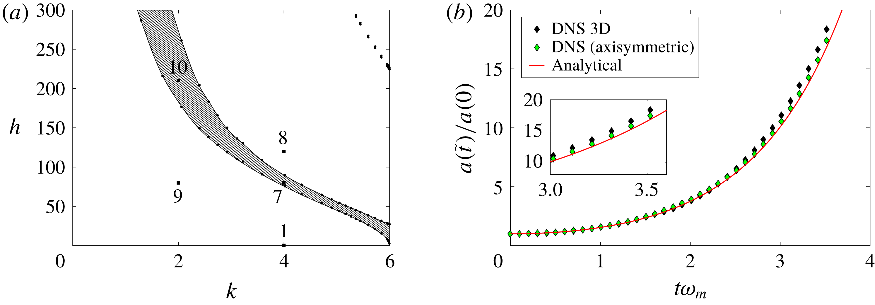
Figure 4 is the master chart and all stability plots on the
 $h$
–
$h$
–
 $k$
plane like the ones shown in figure 6(a–d) are obtained from it. This is done in the following manner. For every point
$k$
plane like the ones shown in figure 6(a–d) are obtained from it. This is done in the following manner. For every point
 $({\mathcal{A}},{\mathcal{B}})$
which lies on the (neutral stability) curves in figure 4, we solve the first and second of equations (3.15), to obtain
$({\mathcal{A}},{\mathcal{B}})$
which lies on the (neutral stability) curves in figure 4, we solve the first and second of equations (3.15), to obtain
 $k$
and
$k$
and
 $h$
, respectively, using the MATLAB (2015) subroutine fzero (see supplementary material 3 which returns a single real root for
$h$
, respectively, using the MATLAB (2015) subroutine fzero (see supplementary material 3 which returns a single real root for
 ${\mathcal{A}}>0$
). The equation containing
${\mathcal{A}}>0$
). The equation containing
 ${\mathcal{A}}$
is used to determine
${\mathcal{A}}$
is used to determine
 $k$
, while that containing
$k$
, while that containing
 ${\mathcal{B}}$
is used for finding
${\mathcal{B}}$
is used for finding
 $h$
, utilising the value of
$h$
, utilising the value of
 $k$
found previously. Thus for every
$k$
found previously. Thus for every
 $({\mathcal{A}},{\mathcal{B}})$
which lies on the neutral stability curves in figure 4, we obtain a corresponding
$({\mathcal{A}},{\mathcal{B}})$
which lies on the neutral stability curves in figure 4, we obtain a corresponding
 $(k,h)$
. The locus of all such points generates figures 6(a), 6(b), 6(c) and 6(d) corresponding to
$(k,h)$
. The locus of all such points generates figures 6(a), 6(b), 6(c) and 6(d) corresponding to
 $m=0,2,3$
and
$m=0,2,3$
and
 $4$
, respectively. We restrict the present study to
$4$
, respectively. We restrict the present study to
 $\unicode[STIX]{x1D70C}^{{\mathcal{I}}}>\unicode[STIX]{x1D70C}^{O}$
(heavier fluid inside the filament) and consequently negative values of
$\unicode[STIX]{x1D70C}^{{\mathcal{I}}}>\unicode[STIX]{x1D70C}^{O}$
(heavier fluid inside the filament) and consequently negative values of
 ${\mathcal{B}}$
need not be considered. Negative values of
${\mathcal{B}}$
need not be considered. Negative values of
 ${\mathcal{A}}$
are considered, as explained below.
${\mathcal{A}}$
are considered, as explained below.
 $$\begin{eqnarray}\displaystyle \left.\begin{array}{@{}c@{}}\displaystyle {\mathcal{A}}\equiv \left(\frac{\unicode[STIX]{x1D714}_{m}(k)}{\unicode[STIX]{x1D6FA}}\right)^{2},\quad {\mathcal{B}}\equiv \frac{h}{2\unicode[STIX]{x1D6FA}^{2}}\left[\frac{\left(\unicode[STIX]{x1D70C}^{{\mathcal{I}}}-\unicode[STIX]{x1D70C}^{O}\right)k}{\unicode[STIX]{x1D70C}^{{\mathcal{I}}}{\displaystyle \frac{\text{I}_{m}(kR_{0})}{\text{I}_{m}^{\prime }(kR_{0})}}-\unicode[STIX]{x1D70C}^{O}{\displaystyle \frac{\text{K}_{m}(kR_{0})}{\text{K}_{m}^{\prime }(kR_{0})}}}\right],\\ \displaystyle \text{with}~\unicode[STIX]{x1D714}_{m}^{2}(k)\equiv \frac{T}{R_{0}^{3}}\left[\frac{kR_{0}\left(k^{2}R_{0}^{2}+m^{2}-1\right)}{\unicode[STIX]{x1D70C}^{{\mathcal{I}}}{\displaystyle \frac{\text{I}_{m}(kR_{0})}{\text{I}_{m}^{\prime }(kR_{0})}}-\unicode[STIX]{x1D70C}^{O}{\displaystyle \frac{\text{K}_{m}(kR_{0})}{\text{K}_{m}^{\prime }(kR_{0})}}}\right].\end{array}\right\} & & \displaystyle\end{eqnarray}$$

Figure 4. The neutral stability curves of (3.8). The tongues separate stable from unstable regions,
 $S$
represents stable,
$S$
represents stable,
 $SH$
subharmonic and
$SH$
subharmonic and
 $H$
harmonic. The dots (see inset on the right) are obtained from Bender & Orszag (Reference Bender and Orszag2010). Note the small dashed region which is stable.
$H$
harmonic. The dots (see inset on the right) are obtained from Bender & Orszag (Reference Bender and Orszag2010). Note the small dashed region which is stable.
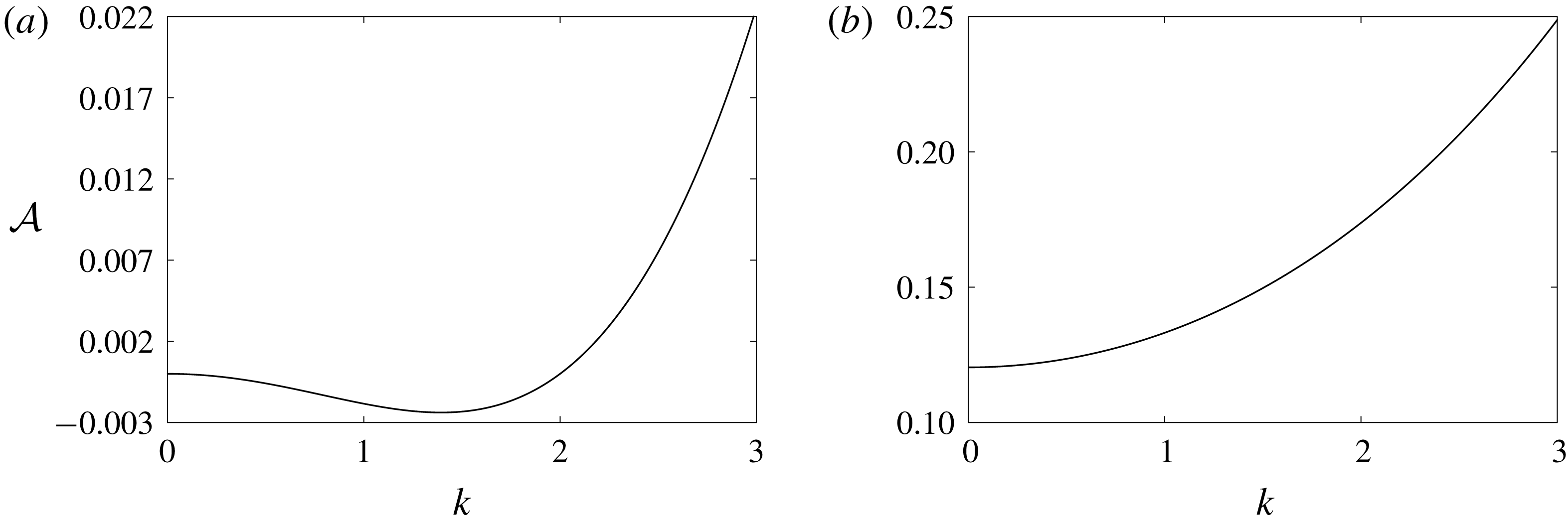
Figure 5.
 ${\mathcal{A}}$
versus
${\mathcal{A}}$
versus
 $k$
for
$k$
for
 $R_{0}=0.5$
,
$R_{0}=0.5$
,
 $T=0.1$
,
$T=0.1$
,
 $\unicode[STIX]{x1D6FA}=2\unicode[STIX]{x03C0}$
,
$\unicode[STIX]{x1D6FA}=2\unicode[STIX]{x03C0}$
,
 $\unicode[STIX]{x1D70C}^{{\mathcal{I}}}=1.0$
,
$\unicode[STIX]{x1D70C}^{{\mathcal{I}}}=1.0$
,
 $\unicode[STIX]{x1D70C}^{O}=0.01$
for (a)
$\unicode[STIX]{x1D70C}^{O}=0.01$
for (a)
 $m=0$
and (b)
$m=0$
and (b)
 $m=2$
. For
$m=2$
. For
 $kR_{0}<1$
and
$kR_{0}<1$
and
 $m=0$
, each negative value of
$m=0$
, each negative value of
 ${\mathcal{A}}$
is associated with two values of
${\mathcal{A}}$
is associated with two values of
 $k$
. Such multivaluedness is not present for
$k$
. Such multivaluedness is not present for
 $m>0$
, as seen in (b) for
$m>0$
, as seen in (b) for
 $m=2$
.
$m=2$
.
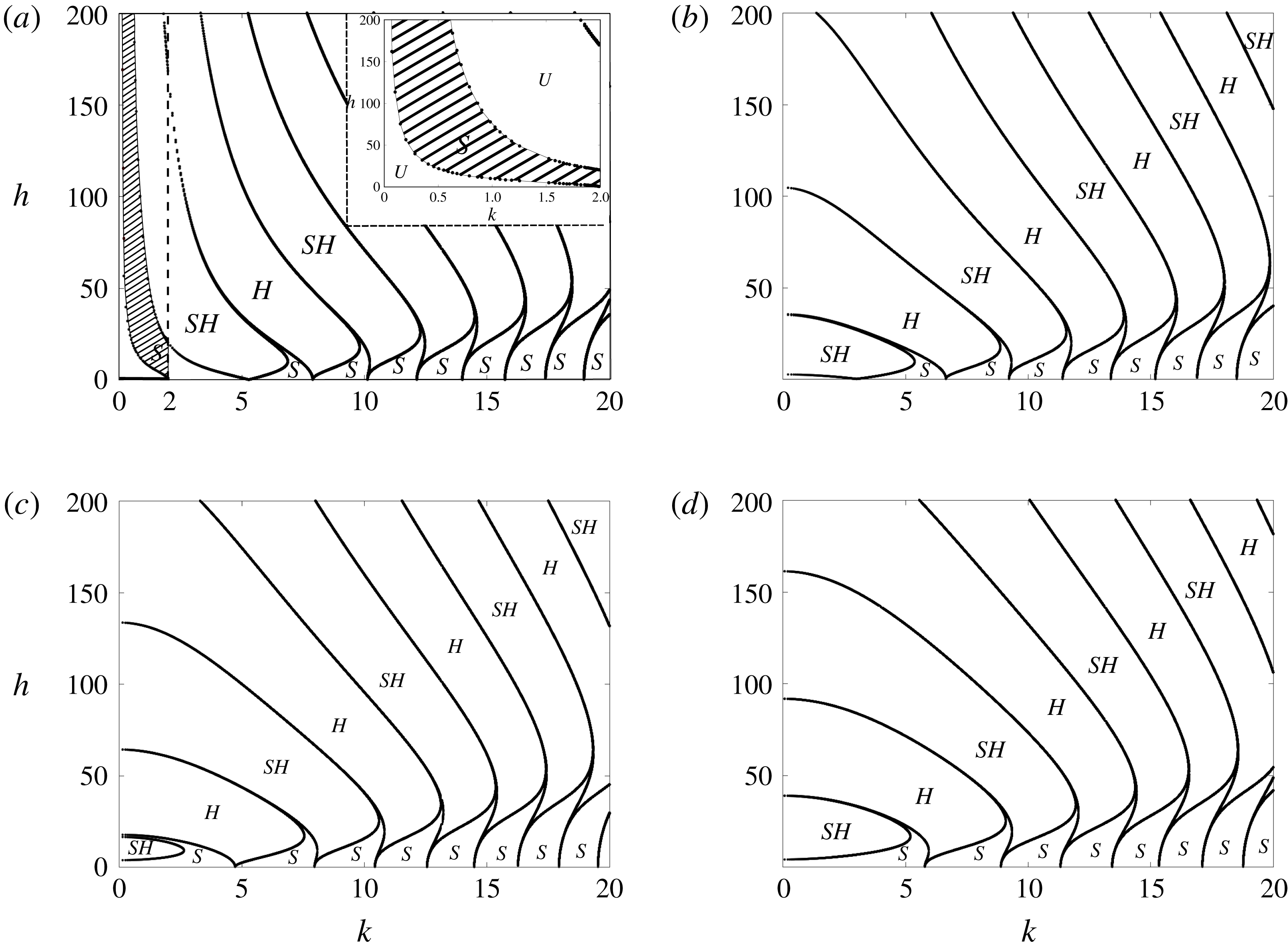
Figure 6. (a) Stable (
 $S$
) and unstable (
$S$
) and unstable (
 $U$
) regions of the Mathieu equation in the
$U$
) regions of the Mathieu equation in the
 ${\mathcal{B}}{-}{\mathcal{A}}$
parametric space using numerical Floquet analysis. (a) (In c.g.s units)
${\mathcal{B}}{-}{\mathcal{A}}$
parametric space using numerical Floquet analysis. (a) (In c.g.s units)
 $R_{0}=0.5$
,
$R_{0}=0.5$
,
 $T=0.1$
,
$T=0.1$
,
 $\unicode[STIX]{x1D6FA}=2\unicode[STIX]{x03C0}$
,
$\unicode[STIX]{x1D6FA}=2\unicode[STIX]{x03C0}$
,
 $\unicode[STIX]{x1D70C}^{{\mathcal{I}}}=1.0$
,
$\unicode[STIX]{x1D70C}^{{\mathcal{I}}}=1.0$
,
 $\unicode[STIX]{x1D70C}^{O}=0.01$
,
$\unicode[STIX]{x1D70C}^{O}=0.01$
,
 $m=0$
. (b–d) Same parameters as (a) except
$m=0$
. (b–d) Same parameters as (a) except
 $m=2$
(b),
$m=2$
(b),
 $m=3$
(c) and
$m=3$
(c) and
 $m=4$
(d).
$m=4$
(d).
 $SH$
: subharmonic and
$SH$
: subharmonic and
 $H$
: harmonic.
$H$
: harmonic.
While finding roots from (3.15) using the procedure described earlier, additional care is necessary for the axisymmetric
 $(m=0)$
case (figure 6
a). This is because, for axisymmetric perturbations
$(m=0)$
case (figure 6
a). This is because, for axisymmetric perturbations
 $(m=0,k\neq 0)$
, the base state is unstable to RP modes satisfying the condition
$(m=0,k\neq 0)$
, the base state is unstable to RP modes satisfying the condition
 $kR_{0}<1$
. Thus in the expression for
$kR_{0}<1$
. Thus in the expression for
 $\unicode[STIX]{x1D714}_{m}^{2}(k)$
in (3.15) with
$\unicode[STIX]{x1D714}_{m}^{2}(k)$
in (3.15) with
 $m=0$
and
$m=0$
and
 $kR_{0}<1$
,
$kR_{0}<1$
,
 $\unicode[STIX]{x1D714}_{m}^{2}(k)$
becomes negative, implying negative values of
$\unicode[STIX]{x1D714}_{m}^{2}(k)$
becomes negative, implying negative values of
 ${\mathcal{A}}$
on the
${\mathcal{A}}$
on the
 ${\mathcal{A}}$
–
${\mathcal{A}}$
–
 ${\mathcal{B}}$
plane in figure 4. In solving (3.15) for negative
${\mathcal{B}}$
plane in figure 4. In solving (3.15) for negative
 ${\mathcal{A}}$
, we adopt a graphical technique for determining the corresponding
${\mathcal{A}}$
, we adopt a graphical technique for determining the corresponding
 $(k,h)$
. It is seen from figure 5(a) that for
$(k,h)$
. It is seen from figure 5(a) that for
 $m=0$
, there are two values of
$m=0$
, there are two values of
 $k$
for every (negative) value of
$k$
for every (negative) value of
 ${\mathcal{A}}$
. We graphically obtain the two positive values of
${\mathcal{A}}$
. We graphically obtain the two positive values of
 $k$
for every negative
$k$
for every negative
 ${\mathcal{A}}$
and then each of these values is used in the second equation in (3.15) to determine a corresponding
${\mathcal{A}}$
and then each of these values is used in the second equation in (3.15) to determine a corresponding
 $h$
. To illustrate this special case, a dashed vertical line is shown in figure 6(a). It is verified from this figure that for
$h$
. To illustrate this special case, a dashed vertical line is shown in figure 6(a). It is verified from this figure that for
 $kR_{0}<1$
, the base state lies in an unstable region and continues to be so even for finite values of
$kR_{0}<1$
, the base state lies in an unstable region and continues to be so even for finite values of
 $h$
, although a stable region (indicated by hash in figure 6
a) also appears. To highlight the instability of the base state for
$h$
, although a stable region (indicated by hash in figure 6
a) also appears. To highlight the instability of the base state for
 $h=0$
, the range
$h=0$
, the range
 $0<k<2$
has been shown in bold in figure 6(a). For
$0<k<2$
has been shown in bold in figure 6(a). For
 $m\geqslant 2$
,
$m\geqslant 2$
,
 ${\mathcal{A}}$
is a single-valued positive function of
${\mathcal{A}}$
is a single-valued positive function of
 $k$
, as seen in figure 5(b), and negative
$k$
, as seen in figure 5(b), and negative
 ${\mathcal{A}}$
need not be considered. The stability charts for
${\mathcal{A}}$
need not be considered. The stability charts for
 $m=2$
, 3 and 4 are shown in figures 6(b), 6(c) and 6(d), respectively (the case
$m=2$
, 3 and 4 are shown in figures 6(b), 6(c) and 6(d), respectively (the case
 $m=1$
translates the centre of mass of the filament and is not of interest for studying oscillations).
$m=1$
translates the centre of mass of the filament and is not of interest for studying oscillations).
4 Numerical simulations
We compare analytical predictions made in earlier sections against numerical results obtained from direct numerical simulations (DNS) of the Euler equations. The simulations have been performed using the open source code Gerris (Popinet Reference Popinet2003, Reference Popinet2009), which solves the incompressible Euler equations with surface tension and an additional time-periodic body force, chosen to be in the radial direction in cylindrical coordinates (see figure 7 c). Interface capturing is done by the Volume of Fluid (VoF) method (Tryggvason, Scardovelli & Zaleski Reference Tryggvason, Scardovelli and Zaleski2011), which also advects the interface. The temporal discretisation is second-order accurate and a Godunov momentum scheme of Bell, Colella & Glaz (Reference Bell, Colella and Glaz1989) is used for advection. A semi-implicit scheme is used to evaluate the velocity and pressure fields (Chorin Reference Chorin1968). For calculation of surface tension force, the continuum surface force (CSF) (Brackbill, Kothe & Zemach Reference Brackbill, Kothe and Zemach1992) model is used. The following equations are solved,
 $$\begin{eqnarray}\displaystyle \frac{\text{D}\boldsymbol{u}}{\text{D}t}=\unicode[STIX]{x1D70C}^{-1}\left\{-\unicode[STIX]{x1D735}p+T\unicode[STIX]{x1D705}\unicode[STIX]{x1D6FF}_{s}\boldsymbol{n}\right\}-h\cos (\unicode[STIX]{x1D6FA}t)\frac{r}{R_{0}}\boldsymbol{e}_{r}, & & \displaystyle\end{eqnarray}$$
 $$\begin{eqnarray}\displaystyle \unicode[STIX]{x1D735}\boldsymbol{\cdot }\boldsymbol{u}=0\quad \text{and}\quad \frac{\unicode[STIX]{x2202}c}{\unicode[STIX]{x2202}t}+\unicode[STIX]{x1D735}\boldsymbol{\cdot }(c\boldsymbol{u})=0, & & \displaystyle\end{eqnarray}$$
where
 $\unicode[STIX]{x1D70C}\equiv c\unicode[STIX]{x1D70C}^{{\mathcal{I}}}+(1-c)\unicode[STIX]{x1D70C}^{O}$
,
$\unicode[STIX]{x1D70C}\equiv c\unicode[STIX]{x1D70C}^{{\mathcal{I}}}+(1-c)\unicode[STIX]{x1D70C}^{O}$
,
 $\boldsymbol{u}$
,
$\boldsymbol{u}$
,
 $p$
,
$p$
,
 $c$
are density, velocity, pressure and volume fraction, respectively. The volume fraction field
$c$
are density, velocity, pressure and volume fraction, respectively. The volume fraction field
 $c$
is chosen to be unity for fluid inside the filament and 0 for fluid outside.
$c$
is chosen to be unity for fluid inside the filament and 0 for fluid outside.
 $T$
is the surface tension coefficient,
$T$
is the surface tension coefficient,
 $\unicode[STIX]{x1D6FF}_{s}$
is a surface delta function (defined as
$\unicode[STIX]{x1D6FF}_{s}$
is a surface delta function (defined as
 $|\unicode[STIX]{x1D735}c|$
, Tryggvason et al. (Reference Tryggvason, Scardovelli and Zaleski2011), see pp. 62),
$|\unicode[STIX]{x1D735}c|$
, Tryggvason et al. (Reference Tryggvason, Scardovelli and Zaleski2011), see pp. 62),
 $\unicode[STIX]{x1D705}\equiv (1/{\mathcal{R}})$
is the local curvature,
$\unicode[STIX]{x1D705}\equiv (1/{\mathcal{R}})$
is the local curvature,
 $\boldsymbol{n}$
is a local unit normal to the interface (see figure 1) and
$\boldsymbol{n}$
is a local unit normal to the interface (see figure 1) and
 $R_{0}$
is the radius of the unperturbed filament. The periodic forcing term in (4.1) is added in the (cylindrical) radial direction
$R_{0}$
is the radius of the unperturbed filament. The periodic forcing term in (4.1) is added in the (cylindrical) radial direction
 $\boldsymbol{e}_{r}$
in both fluids (figure 7
c,d). Gerris has been extensively tested against analytical and experimental predictions (Fuster et al.
Reference Fuster, Bagué, Boeck, Le Moyne, Leboissetier, Popinet, Ray, Scardovelli and Zaleski2009; Popinet Reference Popinet2009; Fuster et al.
Reference Fuster, Matas, Marty, Popinet, Hoepffner, Cartellier and Zaleski2013; Thoraval et al.
Reference Thoraval, Takehara, Etoh and Thoroddsen2013; Dasgupta, Tomar & Govindarajan Reference Dasgupta, Tomar and Govindarajan2015; Tripathi, Sahu & Govindarajan Reference Tripathi, Sahu and Govindarajan2015). With eight parameters
$\boldsymbol{e}_{r}$
in both fluids (figure 7
c,d). Gerris has been extensively tested against analytical and experimental predictions (Fuster et al.
Reference Fuster, Bagué, Boeck, Le Moyne, Leboissetier, Popinet, Ray, Scardovelli and Zaleski2009; Popinet Reference Popinet2009; Fuster et al.
Reference Fuster, Matas, Marty, Popinet, Hoepffner, Cartellier and Zaleski2013; Thoraval et al.
Reference Thoraval, Takehara, Etoh and Thoroddsen2013; Dasgupta, Tomar & Govindarajan Reference Dasgupta, Tomar and Govindarajan2015; Tripathi, Sahu & Govindarajan Reference Tripathi, Sahu and Govindarajan2015). With eight parameters
 $\unicode[STIX]{x1D70C}^{{\mathcal{I}}},\unicode[STIX]{x1D70C}^{O},a(0),R_{0}/m,k,h,\unicode[STIX]{x1D6FA}$
and
$\unicode[STIX]{x1D70C}^{{\mathcal{I}}},\unicode[STIX]{x1D70C}^{O},a(0),R_{0}/m,k,h,\unicode[STIX]{x1D6FA}$
and
 $T$
, from the Buckingham
$T$
, from the Buckingham
 $\unicode[STIX]{x03C0}$
theorem we have five non-dimensional groups. These are chosen to be the density ratio
$\unicode[STIX]{x03C0}$
theorem we have five non-dimensional groups. These are chosen to be the density ratio
 $\unicode[STIX]{x1D70C}_{r}\equiv (\unicode[STIX]{x1D70C}^{{\mathcal{I}}}/\unicode[STIX]{x1D70C}^{O})$
, a non-dimensional measure of axial perturbation amplitude
$\unicode[STIX]{x1D70C}_{r}\equiv (\unicode[STIX]{x1D70C}^{{\mathcal{I}}}/\unicode[STIX]{x1D70C}^{O})$
, a non-dimensional measure of axial perturbation amplitude
 $\unicode[STIX]{x1D716}_{ax}\equiv a(0)k$
and azimuthal perturbation amplitude
$\unicode[STIX]{x1D716}_{ax}\equiv a(0)k$
and azimuthal perturbation amplitude
 $\unicode[STIX]{x1D716}_{az}\equiv (ma(0)/R_{0})$
, a non-dimensional forcing amplitude
$\unicode[STIX]{x1D716}_{az}\equiv (ma(0)/R_{0})$
, a non-dimensional forcing amplitude
 $\unicode[STIX]{x1D6E4}\equiv (\unicode[STIX]{x1D70C}^{{\mathcal{I}}}hR_{0}^{2}/T)$
and a non-dimensional forcing frequency
$\unicode[STIX]{x1D6E4}\equiv (\unicode[STIX]{x1D70C}^{{\mathcal{I}}}hR_{0}^{2}/T)$
and a non-dimensional forcing frequency
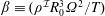 $\unicode[STIX]{x1D6FD}\equiv (\unicode[STIX]{x1D70C}^{{\mathcal{I}}}R_{0}^{3}\unicode[STIX]{x1D6FA}^{2}/T)$
. This choice of non-dimensional parameters is dictated by convention as well as ease of varying these in DNS.
$\unicode[STIX]{x1D6FD}\equiv (\unicode[STIX]{x1D70C}^{{\mathcal{I}}}R_{0}^{3}\unicode[STIX]{x1D6FA}^{2}/T)$
. This choice of non-dimensional parameters is dictated by convention as well as ease of varying these in DNS.
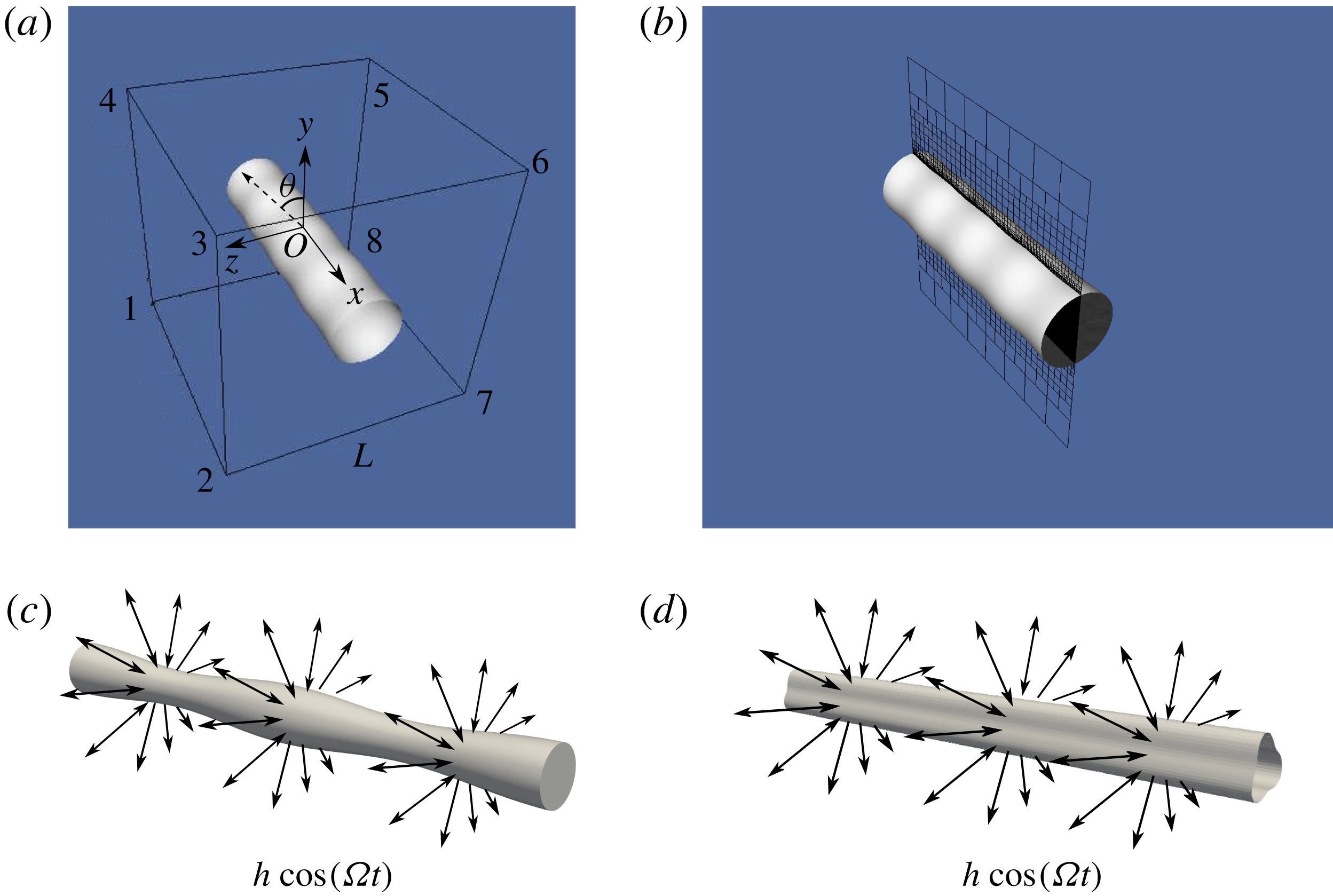
Figure 7. (a) DNS geometry. (b) A sample adaptive grid. (c) An axially perturbed column at
 $t=0$
, i.e.
$t=0$
, i.e.
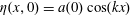 $\unicode[STIX]{x1D702}(x,0)=a(0)\cos (kx)$
. (d) An azimuthally perturbed column at
$\unicode[STIX]{x1D702}(x,0)=a(0)\cos (kx)$
. (d) An azimuthally perturbed column at
 $t=0$
, i.e.
$t=0$
, i.e.
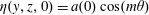 $\unicode[STIX]{x1D702}(y,z,0)=a(0)\cos (m\unicode[STIX]{x1D703})$
with
$\unicode[STIX]{x1D702}(y,z,0)=a(0)\cos (m\unicode[STIX]{x1D703})$
with
 $\unicode[STIX]{x1D703}\equiv \tan ^{-1}(z/y)$
. The radial forcing is depicted only at the surface of the filament and is applied everywhere, as discussed in the text.
$\unicode[STIX]{x1D703}\equiv \tan ^{-1}(z/y)$
. The radial forcing is depicted only at the surface of the filament and is applied everywhere, as discussed in the text.
As all our simulations are in three dimensions, we have used the adaptive grid feature of Gerris (Popinet Reference Popinet2003) to speed up computations (see figure 7
b). A base level refinement of 5 (in powers of two) in every spatial direction was used, implying 32 768 computational cells at the base level. A higher level refinement ranging from 9 to 12 was employed at the interface and the fluid inside the filament. For a typical simulation, the number of grid points along the diameter of the unperturbed filament varied from approximately 100 to 120. The (square) domain size
 $L$
was chosen to be sufficiently large to be able to numerically mimic an unbounded domain. The initial perturbation is chosen to have an integral number of wavelengths in the
$L$
was chosen to be sufficiently large to be able to numerically mimic an unbounded domain. The initial perturbation is chosen to have an integral number of wavelengths in the
 $x$
direction. For applying periodic boundary conditions on the faces 1458 and 2367 in (2.1a,b
), the initial perturbation is chosen such that its extrema are located at the faces 1458 and 2367 (see supplementary material 4). Boundary conditions for the simulations are provided in table 1. The simulation parameters are summarised non-dimensionally in table 2 and dimensionally in supplementary material 1. Amplitude of interface versus time plots are extracted using an open source visualising application Paraview (Ahrens, Geveci & Law Reference Ahrens, Geveci and Law2005). We track the
$x$
direction. For applying periodic boundary conditions on the faces 1458 and 2367 in (2.1a,b
), the initial perturbation is chosen such that its extrema are located at the faces 1458 and 2367 (see supplementary material 4). Boundary conditions for the simulations are provided in table 1. The simulation parameters are summarised non-dimensionally in table 2 and dimensionally in supplementary material 1. Amplitude of interface versus time plots are extracted using an open source visualising application Paraview (Ahrens, Geveci & Law Reference Ahrens, Geveci and Law2005). We track the
 $y$
coordinate of volume fraction contour of level 0.5 with time, at the centre of the domain
$y$
coordinate of volume fraction contour of level 0.5 with time, at the centre of the domain
 $(x=z=0)$
(see figure 7
a). Refer to supplementary material 1 for details. The initial perturbation is chosen to be of the form
$(x=z=0)$
(see figure 7
a). Refer to supplementary material 1 for details. The initial perturbation is chosen to be of the form
 $\unicode[STIX]{x1D702}(x,y,z,0)=a(0)\cos (kx)\cos (m\unicode[STIX]{x1D703})$
, where
$\unicode[STIX]{x1D702}(x,y,z,0)=a(0)\cos (kx)\cos (m\unicode[STIX]{x1D703})$
, where
 $\unicode[STIX]{x1D703}\equiv \tan ^{-1}(z/y)$
(see figure 7
a). The radial forcing is applied to the
$\unicode[STIX]{x1D703}\equiv \tan ^{-1}(z/y)$
(see figure 7
a). The radial forcing is applied to the
 $y$
and
$y$
and
 $z$
momentum equations and is of the form
$z$
momentum equations and is of the form
 $-h\cos (\unicode[STIX]{x1D6FA}t)\cos (\unicode[STIX]{x1D703})(\sqrt{y^{2}+z^{2}}/R_{0})$
in the
$-h\cos (\unicode[STIX]{x1D6FA}t)\cos (\unicode[STIX]{x1D703})(\sqrt{y^{2}+z^{2}}/R_{0})$
in the
 $y$
momentum equation and
$y$
momentum equation and
 $-h\cos (\unicode[STIX]{x1D6FA}t)\sin (\unicode[STIX]{x1D703})(\sqrt{y^{2}+z^{2}}/R_{0})$
in the
$-h\cos (\unicode[STIX]{x1D6FA}t)\sin (\unicode[STIX]{x1D703})(\sqrt{y^{2}+z^{2}}/R_{0})$
in the
 $z$
momentum equation (see figure 7
a,c,d). A variable time step based on CFL as well as a capillary wave time step constraint (Tryggvason et al.
Reference Tryggvason, Scardovelli and Zaleski2011) is used by Gerris. This is
$z$
momentum equation (see figure 7
a,c,d). A variable time step based on CFL as well as a capillary wave time step constraint (Tryggvason et al.
Reference Tryggvason, Scardovelli and Zaleski2011) is used by Gerris. This is
 $\unicode[STIX]{x1D6FF}t=0.8\text{min}[\sqrt{(\unicode[STIX]{x1D70C}^{{\mathcal{I}}}+\unicode[STIX]{x1D70C}^{O})\unicode[STIX]{x1D6E5}^{3}/\unicode[STIX]{x03C0}T},\unicode[STIX]{x1D6E5}/u_{max}]$
, where
$\unicode[STIX]{x1D6FF}t=0.8\text{min}[\sqrt{(\unicode[STIX]{x1D70C}^{{\mathcal{I}}}+\unicode[STIX]{x1D70C}^{O})\unicode[STIX]{x1D6E5}^{3}/\unicode[STIX]{x03C0}T},\unicode[STIX]{x1D6E5}/u_{max}]$
, where
 $\unicode[STIX]{x1D6E5}$
is the grid spacing,
$\unicode[STIX]{x1D6E5}$
is the grid spacing,
 $u_{max}$
is the maximum velocity in the domain and the CFL number is 0.8.
$u_{max}$
is the maximum velocity in the domain and the CFL number is 0.8.
Table 1. Boundary conditions for DNS in figure 7(a).
Table 2. DNS parameters.
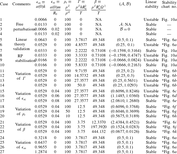
* Denotes figure numbers in supplementary material 1.
5 Results and discussion
As a preliminary validation of the code, we have simulated axisymmetric (
 $m=0$
) free oscillations
$m=0$
) free oscillations
 $(kR_{0}>1)$
as well as the RP instability
$(kR_{0}>1)$
as well as the RP instability
 $(kR_{0}<1)$
by setting
$(kR_{0}<1)$
by setting
 $h=0$
in (4.1) (also see earlier validations in Popinet (Reference Popinet2018)). Gerris has some numerical dissipation (see supplementary material 1 for an estimate) but this is not found to be substantial over the first few cycles. DNS results are compared to predictions from expression (3.5). Cases 1, 2, 3 and 4 in table 2 provide non-dimensional parameter values for these simulations (see supplementary material 1 for the table of corresponding dimensional values). The dispersion relation (3.5) predicts the RP instability for
$h=0$
in (4.1) (also see earlier validations in Popinet (Reference Popinet2018)). Gerris has some numerical dissipation (see supplementary material 1 for an estimate) but this is not found to be substantial over the first few cycles. DNS results are compared to predictions from expression (3.5). Cases 1, 2, 3 and 4 in table 2 provide non-dimensional parameter values for these simulations (see supplementary material 1 for the table of corresponding dimensional values). The dispersion relation (3.5) predicts the RP instability for
 $kR_{0}<1,m=0$
, while for
$kR_{0}<1,m=0$
, while for
 $m\geqslant 2$
, harmonic oscillations of frequency
$m\geqslant 2$
, harmonic oscillations of frequency
 $\unicode[STIX]{x1D714}_{m}(k)$
are predicted, irrespective of the value of
$\unicode[STIX]{x1D714}_{m}(k)$
are predicted, irrespective of the value of
 $kR_{0}$
. This is validated in figure 8(a), where the non-dimensional amplitude
$kR_{0}$
. This is validated in figure 8(a), where the non-dimensional amplitude
 $a(t)/a(0)$
is plotted against non-dimensional time
$a(t)/a(0)$
is plotted against non-dimensional time
 $t\unicode[STIX]{x1D714}_{m}(k)$
. Cases 2, 3 and 4 in table 2 correspond to
$t\unicode[STIX]{x1D714}_{m}(k)$
. Cases 2, 3 and 4 in table 2 correspond to
 $(m=0,kR_{0}\approx 1.333),(m=2,kR_{0}\approx 0.667)$
and
$(m=0,kR_{0}\approx 1.333),(m=2,kR_{0}\approx 0.667)$
and
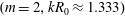 $(m=2,kR_{0}\approx 1.333)$
, respectively. For all the three cases, undamped oscillations are observed with a good agreement between the frequency obtained in DNS and the analytically calculated frequency from relation (3.5). For Case 1 in figure 8(a), relation (3.5) predicts exponential growth due to the RP instability, and this is validated from DNS. In figure 8(b), we show the disintegration of the filament due to the instability in Case 1 and subsequent filament and droplet formation. Note that for DNS of all cases reported in this study, the perturbations were initiated on the interface of the filament with zero velocity field everywhere in the domain.
$(m=2,kR_{0}\approx 1.333)$
, respectively. For all the three cases, undamped oscillations are observed with a good agreement between the frequency obtained in DNS and the analytically calculated frequency from relation (3.5). For Case 1 in figure 8(a), relation (3.5) predicts exponential growth due to the RP instability, and this is validated from DNS. In figure 8(b), we show the disintegration of the filament due to the instability in Case 1 and subsequent filament and droplet formation. Note that for DNS of all cases reported in this study, the perturbations were initiated on the interface of the filament with zero velocity field everywhere in the domain.

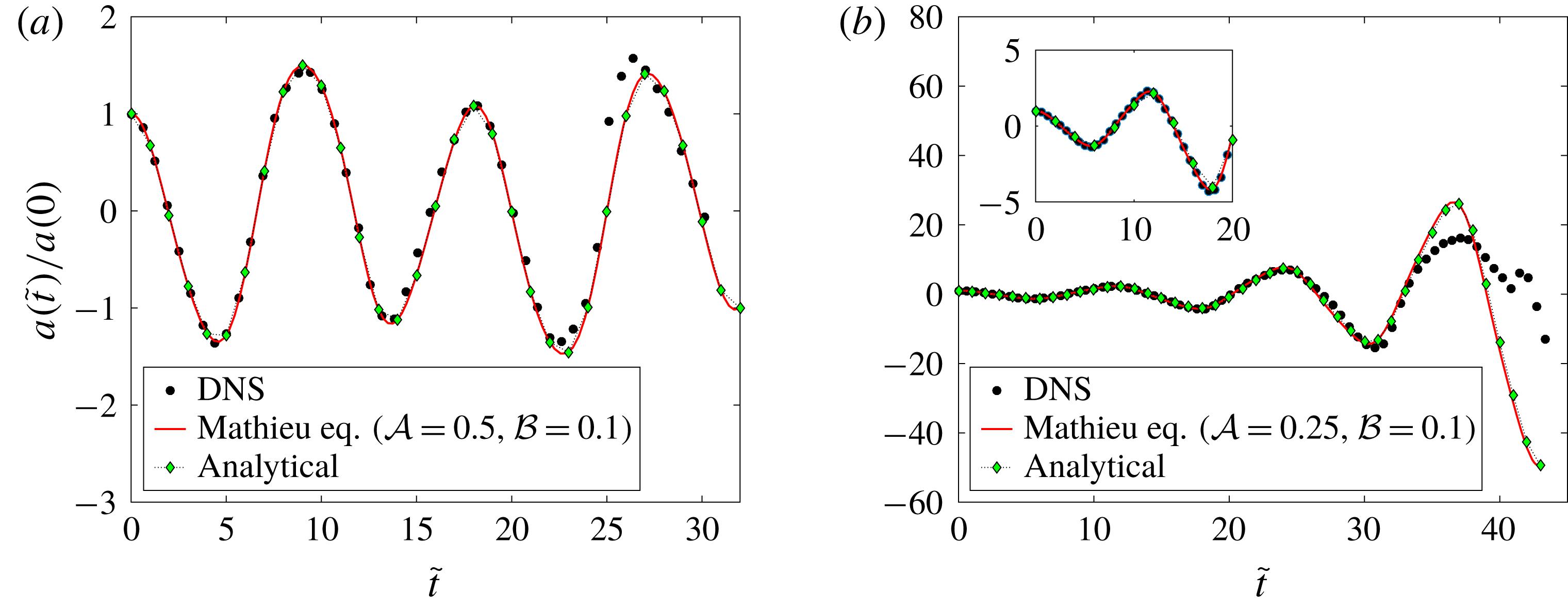
Figure 9. (a) Comparison of DNS results (case 5 in table 2) with numerical solution to (3.8) and perturbative solution from (A 1) with
 $r=1.2821$
and
$r=1.2821$
and
 $\unicode[STIX]{x1D6E9}=0$
. (b) Comparison of DNS results (case 6 in table 2) with numerical solution to (3.8) and perturbative solution from (A 2) with
$\unicode[STIX]{x1D6E9}=0$
. (b) Comparison of DNS results (case 6 in table 2) with numerical solution to (3.8) and perturbative solution from (A 2) with
 $K_{1}=-K_{2}=0.238095$
. The values of
$K_{1}=-K_{2}=0.238095$
. The values of
 $r,\unicode[STIX]{x1D6E9}$
in (a) and
$r,\unicode[STIX]{x1D6E9}$
in (a) and
 $K_{1},K_{2}$
in (b) are obtained from
$K_{1},K_{2}$
in (b) are obtained from
 $a(0)=1$
and
$a(0)=1$
and
 ${\dot{a}}(0)=0$
.
${\dot{a}}(0)=0$
.

In figure 9(a,b), we compare DNS data with numerical solutions to (3.8) using the MATLAB (2015) solver ode45 and the perturbative solutions given by expressions (A 1) and (A 2) in appendix A. Figure 9(a) corresponds to the linearly stable case 5 in table 2, while figure 9(b) corresponds to the linearly unstable case 6. In both cases, the simulation parameters were chosen to ensure that
 ${\mathcal{B}}\ll 1$
, thus enabling comparison with the perturbative solutions (A 1) and (A 2). Note that while solving the Mathieu equation (3.8), we have used the initial conditions
${\mathcal{B}}\ll 1$
, thus enabling comparison with the perturbative solutions (A 1) and (A 2). Note that while solving the Mathieu equation (3.8), we have used the initial conditions
 $a(0)=1$
and
$a(0)=1$
and
 ${\dot{a}}(0)=0$
in all cases. For the perturbative solutions, equation (A 1) and (A 2), these two initial conditions are used to determine the value of
${\dot{a}}(0)=0$
in all cases. For the perturbative solutions, equation (A 1) and (A 2), these two initial conditions are used to determine the value of
 $r,\unicode[STIX]{x1D6E9}$
and
$r,\unicode[STIX]{x1D6E9}$
and
 $K_{1}$
,
$K_{1}$
,
 $K_{2}$
, respectively. A good match with linearised predictions is seen in both cases. In the unstable case in figure 9(b), it is seen that the DNS amplitude follows an initial exponential growth but eventually saturates after few cycles, leading to disagreement with the solution to the Mathieu equation (3.8), which has no mechanism for saturation.
$K_{2}$
, respectively. A good match with linearised predictions is seen in both cases. In the unstable case in figure 9(b), it is seen that the DNS amplitude follows an initial exponential growth but eventually saturates after few cycles, leading to disagreement with the solution to the Mathieu equation (3.8), which has no mechanism for saturation.
5.1 RP modes in the presence of forcing
We saw earlier in § 3.2.1 (see figure 6(a)) that, for a given value of forcing, a range of modes which are RP unstable (i.e.
 $m=0,kR_{0}<1$
) in the absence of forcing can be stabilised through forcing in a small range of forcing amplitudes. We test this prediction here. Figure 10(a) is a stability chart for the special region
$m=0,kR_{0}<1$
) in the absence of forcing can be stabilised through forcing in a small range of forcing amplitudes. We test this prediction here. Figure 10(a) is a stability chart for the special region
 $kR_{0}<1$
(here
$kR_{0}<1$
(here
 $0<k<6.0$
with
$0<k<6.0$
with
 $R_{0}=1/6$
). The white region in this chart corresponds to unstable behaviour while the hashed region is predicted from linear theory to be stable. We have chosen five simulations (cases 1, 7, 8, 9, 10 in table 2) for validating these analytical predictions. Case 1 is for zero forcing
$R_{0}=1/6$
). The white region in this chart corresponds to unstable behaviour while the hashed region is predicted from linear theory to be stable. We have chosen five simulations (cases 1, 7, 8, 9, 10 in table 2) for validating these analytical predictions. Case 1 is for zero forcing
 $(h=0)$
and is RP unstable. Cases 7 and 8 have the same perturbation wavenumber as 1, and are stable and unstable, respectively. Figure 10(b) shows the time signal extracted from axisymmetric as well as (3D) DNS for case 1. Expectedly, it is RP unstable with exponential growth at early times, agreeing very well with linear predictions. There is disagreement with linearised predictions after
$(h=0)$
and is RP unstable. Cases 7 and 8 have the same perturbation wavenumber as 1, and are stable and unstable, respectively. Figure 10(b) shows the time signal extracted from axisymmetric as well as (3D) DNS for case 1. Expectedly, it is RP unstable with exponential growth at early times, agreeing very well with linear predictions. There is disagreement with linearised predictions after
 $t\unicode[STIX]{x1D714}_{m}>2.5$
due to nonlinear effects. Note from the inset in figure 10(b) that, while the onset of perceptible nonlinear effects occurs around the same time (
$t\unicode[STIX]{x1D714}_{m}>2.5$
due to nonlinear effects. Note from the inset in figure 10(b) that, while the onset of perceptible nonlinear effects occurs around the same time (
 $t\unicode[STIX]{x1D714}_{m}\approx 2.5$
) for both axisymmetric and 3D DNS, substantial deviations are seen between the two signals afterwards, occurring primarily due to non-axisymmetric effects.
$t\unicode[STIX]{x1D714}_{m}\approx 2.5$
) for both axisymmetric and 3D DNS, substantial deviations are seen between the two signals afterwards, occurring primarily due to non-axisymmetric effects.

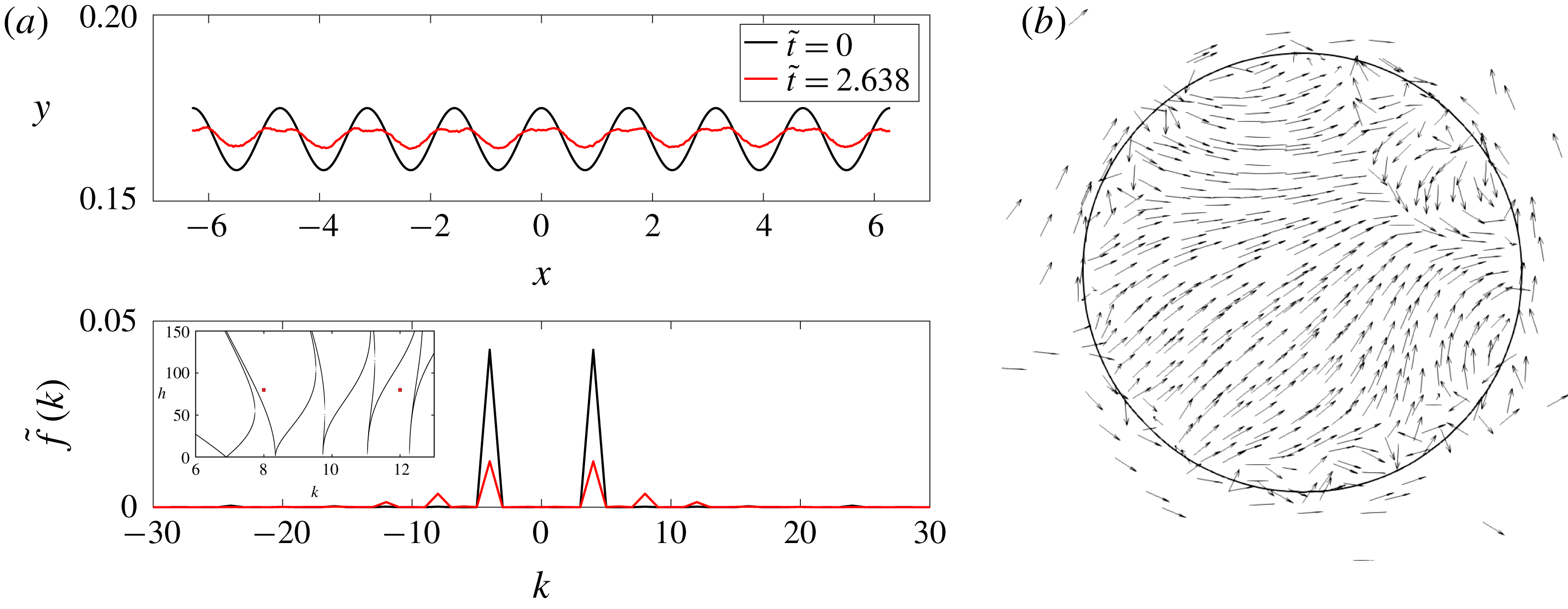
Figure 12. Case 7 from table 2. (a) Top: interface cross-section on the
 $x$
–
$x$
–
 $y$
plane (
$y$
plane (
 $z=0$
). Bottom: Fourier transform of the interface. (Inset) Stability chart. (b) Instantaneous velocity vectors on a cross-section of the interface on the
$z=0$
). Bottom: Fourier transform of the interface. (Inset) Stability chart. (b) Instantaneous velocity vectors on a cross-section of the interface on the
 $z$
–
$z$
–
 $y$
plane (
$y$
plane (
 $x=0$
).
$x=0$
).
Case 7 in figure 10(a) has the same perturbation wavenumber as Case 1 but is theoretically predicted to be stabilised through forcing. An important point to note here is that the stabilisation of axisymmetric RP modes in figure 10(a) is predicted to be purely through (axisymmetric) forcing, i.e. the forcing function
 $G(r,t)$
in our simulations is independent of
$G(r,t)$
in our simulations is independent of
 $\unicode[STIX]{x1D703}$
. This is in contrast to the unforced case (
$\unicode[STIX]{x1D703}$
. This is in contrast to the unforced case (
 $h=0$
), where the RP instability can be suppressed only through 3D initial perturbations (
$h=0$
), where the RP instability can be suppressed only through 3D initial perturbations (
 $m\geqslant 2$
). The predicted stabilisation of Case 7 is indeed observed in DNS at early times in figure 11(a), where both axisymmetric and 3D DNS show stabilisation and agreement with the solution to the Mathieu equation. This agreement is however short-lived, as nonlinear effects start to appear around
$m\geqslant 2$
). The predicted stabilisation of Case 7 is indeed observed in DNS at early times in figure 11(a), where both axisymmetric and 3D DNS show stabilisation and agreement with the solution to the Mathieu equation. This agreement is however short-lived, as nonlinear effects start to appear around
 $\tilde{t}\approx 2.5$
, producing instability. Interestingly, this instability can be understood from our linear theory. Figure 12(a) (upper panel) shows a slice of the cylindrical filament on the
$\tilde{t}\approx 2.5$
, producing instability. Interestingly, this instability can be understood from our linear theory. Figure 12(a) (upper panel) shows a slice of the cylindrical filament on the
 $x-y$
(
$x-y$
(
 $z=0$
) plane obtained from 3D DNS at
$z=0$
) plane obtained from 3D DNS at
 $\tilde{t}=0$
and 2.638 (see arrow in figure 11(a)). It is seen that at
$\tilde{t}=0$
and 2.638 (see arrow in figure 11(a)). It is seen that at
 $\tilde{t}=2.638$
the interface does not resemble a single Fourier mode, although we had started with a single wavenumber
$\tilde{t}=2.638$
the interface does not resemble a single Fourier mode, although we had started with a single wavenumber
 $k=4$
at
$k=4$
at
 $\tilde{t}=0$
. The lower panel shows the Fourier transform
$\tilde{t}=0$
. The lower panel shows the Fourier transform
 $\tilde{f}(k)$
of the interface in the upper panel, revealing the formation of two additional Fourier modes, viz.
$\tilde{f}(k)$
of the interface in the upper panel, revealing the formation of two additional Fourier modes, viz.
 $k=8$
and 12, due to nonlinearity at
$k=8$
and 12, due to nonlinearity at
 $\tilde{t}=2.638$
. This is in contrast to the Fourier transform of the interface at
$\tilde{t}=2.638$
. This is in contrast to the Fourier transform of the interface at
 $\tilde{t}=0$
, where there is a single peak corresponding to a Fourier mode
$\tilde{t}=0$
, where there is a single peak corresponding to a Fourier mode
 $k=4$
. The inset of the figure shows the corresponding stability chart, with the additional wavenumbers produced due to nonlinearity shown as points. It is clearly seen that at this forcing amplitude, the
$k=4$
. The inset of the figure shows the corresponding stability chart, with the additional wavenumbers produced due to nonlinearity shown as points. It is clearly seen that at this forcing amplitude, the
 $k=8$
wavenumber lies inside a tongue and is unstable. This is the origin of the destabilisation seen in figure 11(a). Note that while the time of onset of nonlinearity is roughly the same in both axisymmetric and 3D DNS in figure 11(a), the subsequent temporal routes are very different, as seen in the difference between time signals. Figure 12(b) shows a slice of the filament at
$k=8$
wavenumber lies inside a tongue and is unstable. This is the origin of the destabilisation seen in figure 11(a). Note that while the time of onset of nonlinearity is roughly the same in both axisymmetric and 3D DNS in figure 11(a), the subsequent temporal routes are very different, as seen in the difference between time signals. Figure 12(b) shows a slice of the filament at
 $x=0$
and
$x=0$
and
 $\tilde{t}=2.638$
with the instantaneous velocity vectors inside the filament (those outside have not been plotted). The presence of substantial azimuthal components in the velocity vectors shows that non-axisymmetric effects arising due to nonlinearity cause the 3D DNS to temporally evolve differently from the axisymmetric one. Figure 11(b) corresponds to Case 8 in the stability chart (figure 10
a) and is predicted to be linearly unstable. Once again, a good match at early times is observed, although around
$\tilde{t}=2.638$
with the instantaneous velocity vectors inside the filament (those outside have not been plotted). The presence of substantial azimuthal components in the velocity vectors shows that non-axisymmetric effects arising due to nonlinearity cause the 3D DNS to temporally evolve differently from the axisymmetric one. Figure 11(b) corresponds to Case 8 in the stability chart (figure 10
a) and is predicted to be linearly unstable. Once again, a good match at early times is observed, although around
 $\tilde{t}\approx 3$
nonlinear effects lead to disagreement with linear predictions. As a further validation of our linearised predictions, Case 9 and 10 in the stability chart (figure 10
a) (for
$\tilde{t}\approx 3$
nonlinear effects lead to disagreement with linear predictions. As a further validation of our linearised predictions, Case 9 and 10 in the stability chart (figure 10
a) (for
 $k=2$
) are predicted to be linearly unstable and stable, respectively, in the presence of forcing. This prediction is seen to be validated in figure 13(a,b) (see inset of both figures for linearised predictions). Once again at early times, both axisymmetric and 3D DNS show good agreement with the Mathieu solution but show disagreement at later times due to the production of higher modes and non-axisymmetric effects.
$k=2$
) are predicted to be linearly unstable and stable, respectively, in the presence of forcing. This prediction is seen to be validated in figure 13(a,b) (see inset of both figures for linearised predictions). Once again at early times, both axisymmetric and 3D DNS show good agreement with the Mathieu solution but show disagreement at later times due to the production of higher modes and non-axisymmetric effects.
It is worthwhile to ask if the predicted linear stabilisation of RP modes via forcing may be observed in experiments. We hypothesise that the effect of viscous damping will have a strong suppressing effect on the emergence of the higher wavenumbers and subsequent destabilisation seen in our inviscid DNS. Consequently, for a viscous fluid we anticipate that the stabilisation via forcing predicted in this study may indeed be observed for much longer times than are seen in our inviscid results. Note that the stability boundaries of figure 10(a) will also be modified due to viscosity.

5.2 Parametric studies
For visualisation of the instantaneous surface of the cylindrical filament, we have provided a collage of 3D images in figures 14–17 which correspond to cases 6, 12, 15 and 16 in table 2, respectively. Movies corresponding to these four collages are provided as supplementary movies 1, 2, 3 and 4 respectively. Figure 14 shows the temporal evolution of unstable Faraday waves at the cylindrical interface (case 6). Nonlinear effects become distinctly visible at
 $\tilde{t}=14\unicode[STIX]{x03C0}$
. Two-dimensional slices of the cylindrical filament on the
$\tilde{t}=14\unicode[STIX]{x03C0}$
. Two-dimensional slices of the cylindrical filament on the
 $x$
–
$x$
–
 $y$
plane (at
$y$
plane (at
 $z=0$
) and
$z=0$
) and
 $z$
–
$z$
–
 $y$
(at
$y$
(at
 $x=0$
) plane (see geometry in figure 7
a) are shown in figure 18(a,b). At
$x=0$
) plane (see geometry in figure 7
a) are shown in figure 18(a,b). At
 $\tilde{t}=14\unicode[STIX]{x03C0}$
nonlinear effects are clearly seen in the axial direction as a slice of the interface on the
$\tilde{t}=14\unicode[STIX]{x03C0}$
nonlinear effects are clearly seen in the axial direction as a slice of the interface on the
 $x$
–
$x$
–
 $y$
plane does not resemble a cosine mode. Interestingly, the slice on the
$y$
plane does not resemble a cosine mode. Interestingly, the slice on the
 $z$
–
$z$
–
 $y$
plane shows that the interface remains circular to a good approximation. Figure 18(c) shows the instantaneous streamlines for the snapshot corresponding to non-dimensional time
$y$
plane shows that the interface remains circular to a good approximation. Figure 18(c) shows the instantaneous streamlines for the snapshot corresponding to non-dimensional time
 $\tilde{t}=14\unicode[STIX]{x03C0}$
. For ease of visualisation, the thickness of the streamlines have been increased, giving them the appearance of tubes. It is seen that, except at the necks of the filament, velocity vectors in the azimuthal
$\tilde{t}=14\unicode[STIX]{x03C0}$
. For ease of visualisation, the thickness of the streamlines have been increased, giving them the appearance of tubes. It is seen that, except at the necks of the filament, velocity vectors in the azimuthal
 $(\unicode[STIX]{x1D703})$
direction are small. Figure 15 shows a collage of instantaneous snapshots for Case 12 in table 2. This is also a linearly unstable case, albeit for higher values of forcing parameter
$(\unicode[STIX]{x1D703})$
direction are small. Figure 15 shows a collage of instantaneous snapshots for Case 12 in table 2. This is also a linearly unstable case, albeit for higher values of forcing parameter
 $h$
compared to case 6. We see the clear emergence of sheet-like structures after three forcing time periods
$h$
compared to case 6. We see the clear emergence of sheet-like structures after three forcing time periods
 $(\tilde{t}=6\unicode[STIX]{x03C0})$
. The disintegration seen at
$(\tilde{t}=6\unicode[STIX]{x03C0})$
. The disintegration seen at
 $\tilde{t}=6.8\unicode[STIX]{x03C0}$
is an outcome of the sheet closing upon the filament while shrinking (see supplementary movie 2 for details). The corresponding instantaneous slices on the
$\tilde{t}=6.8\unicode[STIX]{x03C0}$
is an outcome of the sheet closing upon the filament while shrinking (see supplementary movie 2 for details). The corresponding instantaneous slices on the
 $x$
–
$x$
–
 $y$
and
$y$
and
 $z$
–
$z$
–
 $y$
planes are seen in figure 19. The tiny dots, seen at
$y$
planes are seen in figure 19. The tiny dots, seen at
 $\tilde{t}=6.6\unicode[STIX]{x03C0}$
inside and outside the filament in figure 19, correspond to droplets and bubbles formed due to pinch-off and entrapment of surrounding fluid inside the filament respectively (see supplementary movie 2). Due to a larger forcing amplitude, nonlinear effects are visible earlier in figure 15 when compared to figure 14. Note that both the simulations presented in figures 14 and 15 are initiated with axisymmetric initial perturbations (i.e.
$\tilde{t}=6.6\unicode[STIX]{x03C0}$
inside and outside the filament in figure 19, correspond to droplets and bubbles formed due to pinch-off and entrapment of surrounding fluid inside the filament respectively (see supplementary movie 2). Due to a larger forcing amplitude, nonlinear effects are visible earlier in figure 15 when compared to figure 14. Note that both the simulations presented in figures 14 and 15 are initiated with axisymmetric initial perturbations (i.e.
 $m=0,k\neq 0$
).
$m=0,k\neq 0$
).
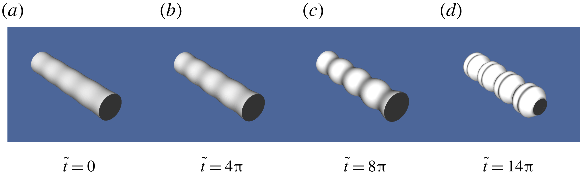
Figure 14. Case 6 in table 2.
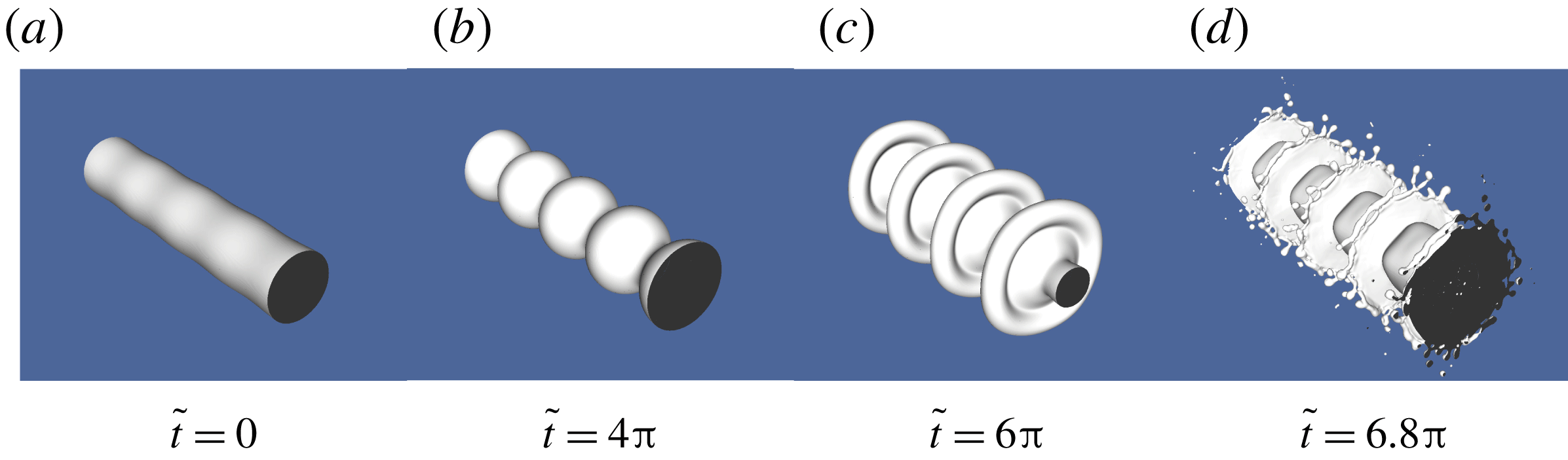
Figure 15. Case 12 in table 2.
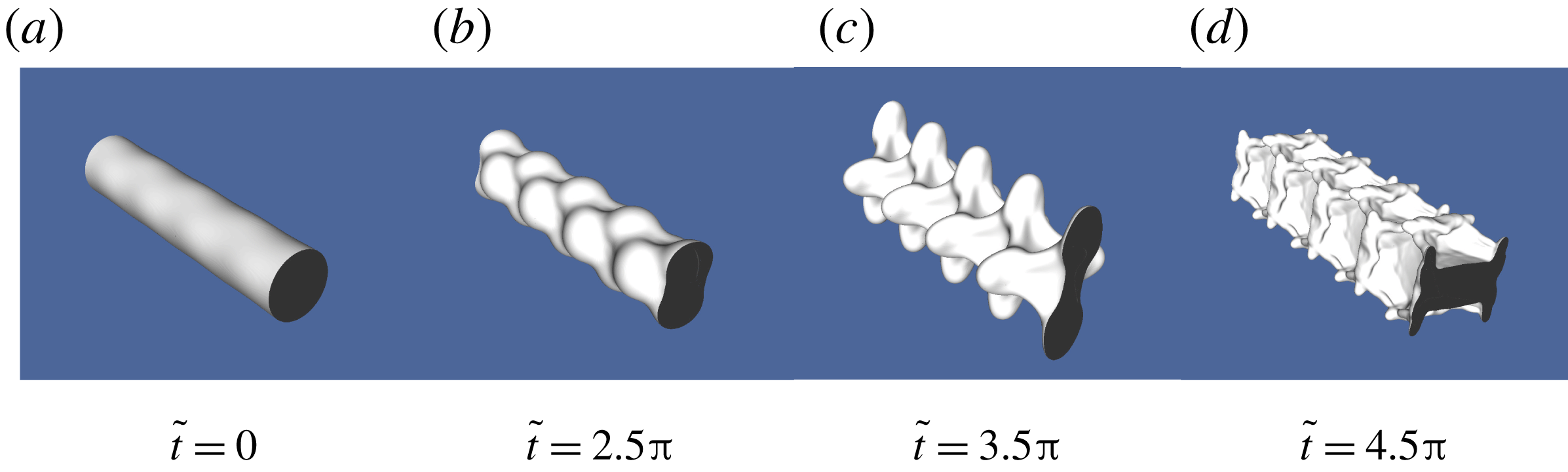
Figure 16. Case 15 in table 2.
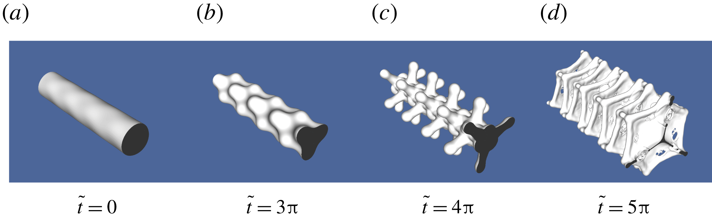
Figure 17. Case 16 in table 2.
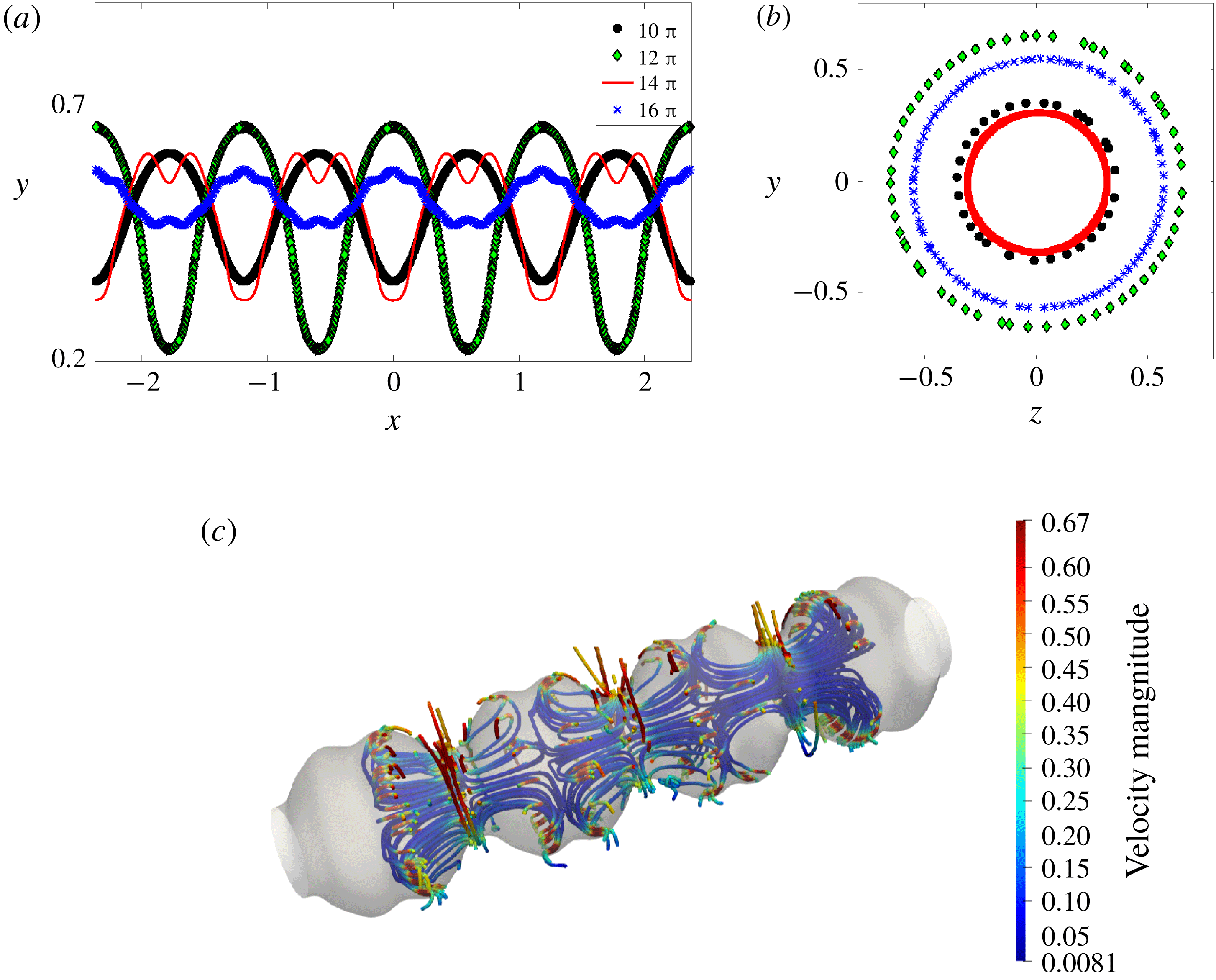
Figure 18. For case 6 in table 2, instantaneous interface profiles on the (a)
 $x$
–
$x$
–
 $y$
plane and (b)
$y$
plane and (b)
 $z$
–
$z$
–
 $y$
plane. (c) Instantaneous streamlines for the profile corresponding to
$y$
plane. (c) Instantaneous streamlines for the profile corresponding to
 $\tilde{t}=14\unicode[STIX]{x03C0}$
.
$\tilde{t}=14\unicode[STIX]{x03C0}$
.
The effects of 3D initial perturbations (
 $m\neq 0,k\neq 0$
) are seen in the collage provided in figures 16 and 17, where in addition to axial perturbation
$m\neq 0,k\neq 0$
) are seen in the collage provided in figures 16 and 17, where in addition to axial perturbation
 $k$
, azimuthal perturbation of wavenumber
$k$
, azimuthal perturbation of wavenumber
 $m=2$
and
$m=2$
and
 $m=3$
are also provided at time
$m=3$
are also provided at time
 $t=0$
, respectively. It is seen in both these cases that the instantaneous (nonlinear) patterns which appear retain memory of the symmetry of the initial perturbation. Figures 16 and 17 panel (c) shows two and three lobes, respectively, retaining the memory of the initial perturbation. In both cases, the instability eventually leads to formation of sheets and their fragmentation, albeit in very different ways. The corresponding instantaneous interface profiles on the
$t=0$
, respectively. It is seen in both these cases that the instantaneous (nonlinear) patterns which appear retain memory of the symmetry of the initial perturbation. Figures 16 and 17 panel (c) shows two and three lobes, respectively, retaining the memory of the initial perturbation. In both cases, the instability eventually leads to formation of sheets and their fragmentation, albeit in very different ways. The corresponding instantaneous interface profiles on the
 $x$
–
$x$
–
 $y$
and
$y$
and
 $z$
–
$z$
–
 $y$
planes are shown in figures 20(a,b) and 21(a,b), respectively. Figure 21(c) shows the instantaneous streamlines corresponding to
$y$
planes are shown in figures 20(a,b) and 21(a,b), respectively. Figure 21(c) shows the instantaneous streamlines corresponding to
 $\tilde{t}=3\unicode[STIX]{x03C0}$
in figure 21(a). Due to the initial 3D nature of the perturbation, 3D velocity fields are clearly seen.
$\tilde{t}=3\unicode[STIX]{x03C0}$
in figure 21(a). Due to the initial 3D nature of the perturbation, 3D velocity fields are clearly seen.
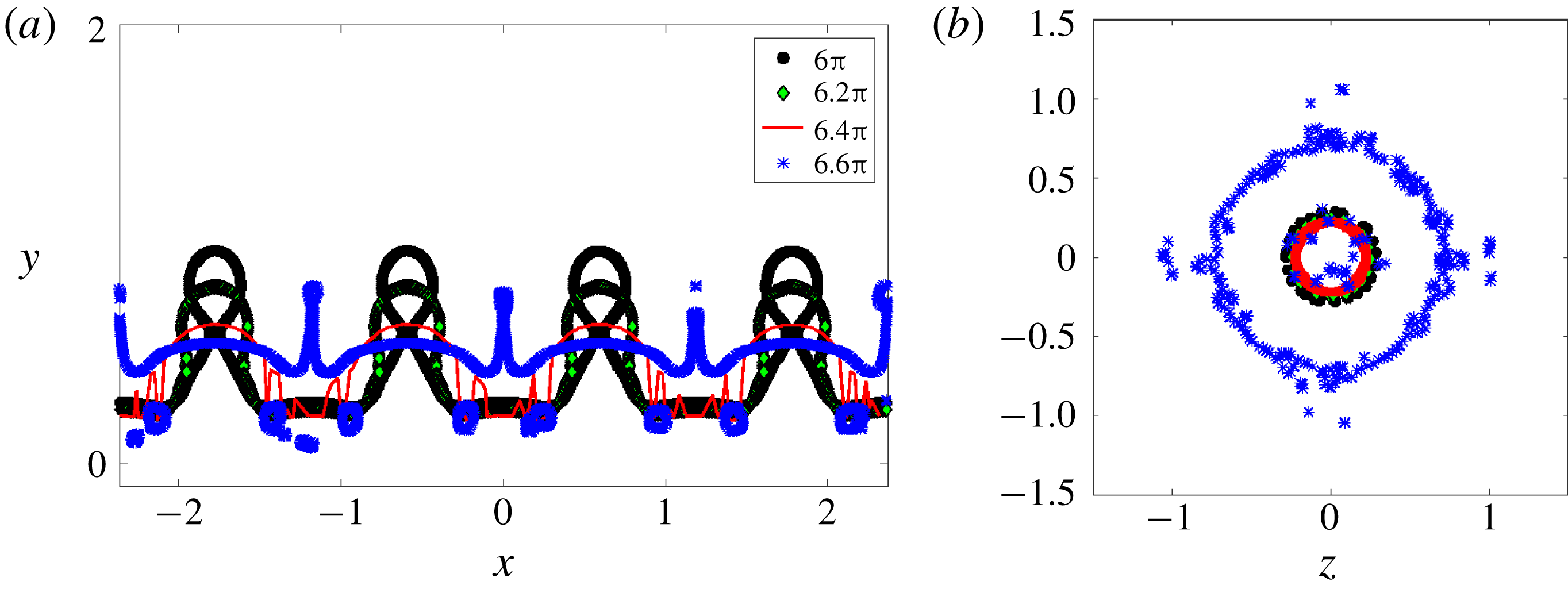
Figure 19. For case 12 in table 2, instantaneous interface profiles on the (a)
 $x$
–
$x$
–
 $y$
plane and (b)
$y$
plane and (b)
 $z$
–
$z$
–
 $y$
plane.
$y$
plane.
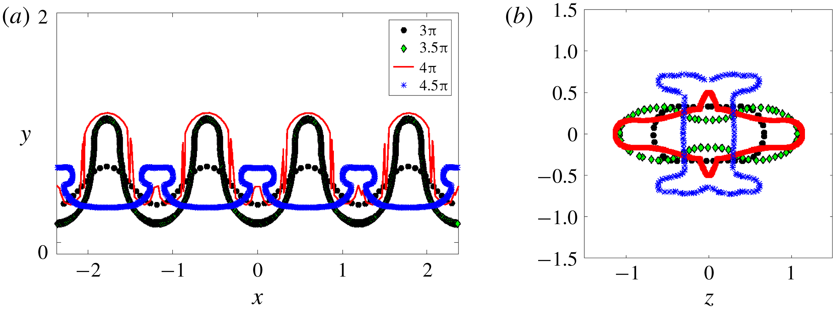
Figure 20. For case 15 in table 2, instantaneous interface profiles on the (a)
 $x$
–
$x$
–
 $y$
plane and (b)
$y$
plane and (b)
 $z$
–
$z$
–
 $y$
plane.
$y$
plane.
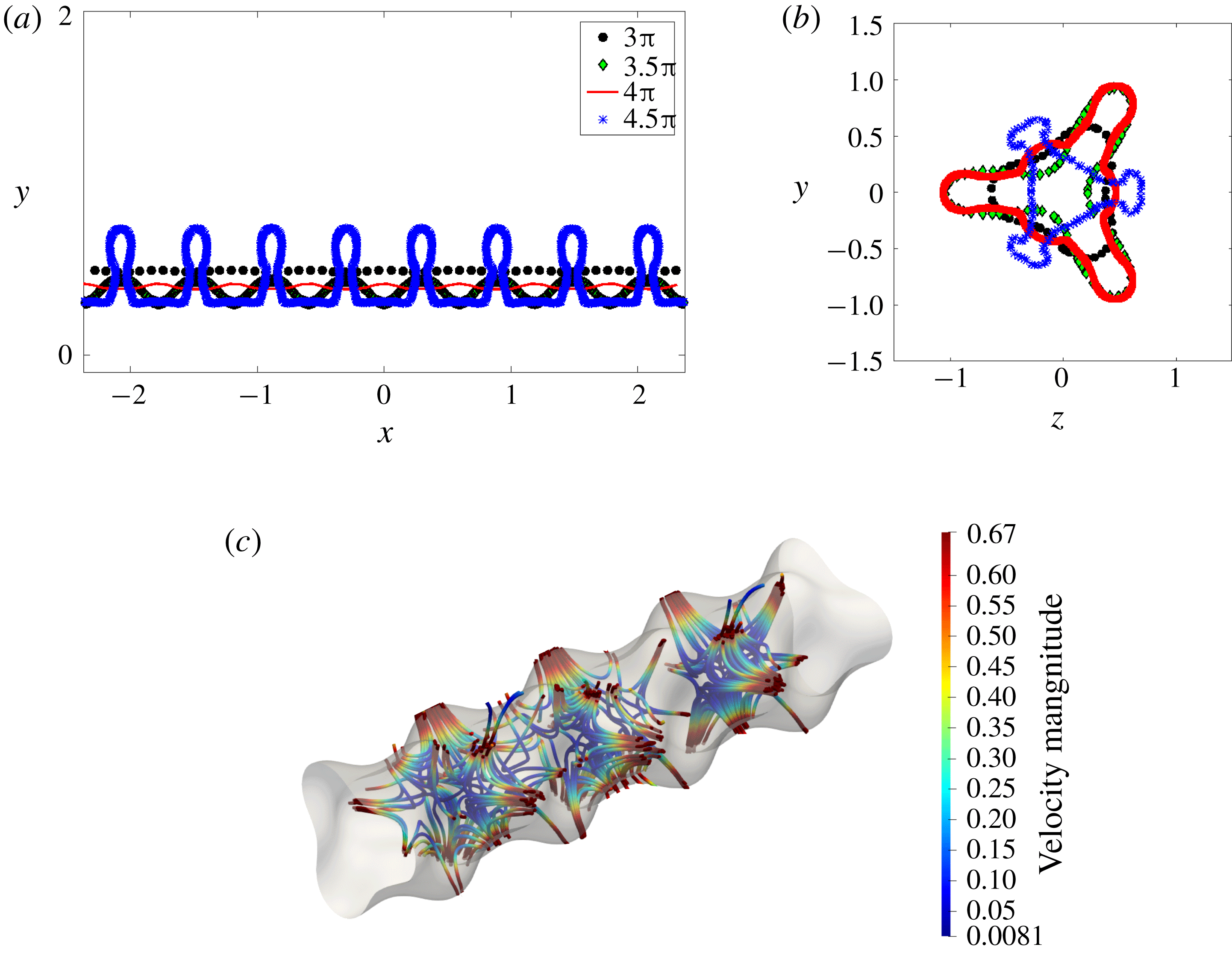
Figure 21. For case 16 in table 2, instantaneous interface profiles on the (a)
 $x$
–
$x$
–
 $y$
plane and (b)
$y$
plane and (b)
 $z$
–
$z$
–
 $y$
plane. (c) Instantaneous streamlines for the profile corresponding to
$y$
plane. (c) Instantaneous streamlines for the profile corresponding to
 $\tilde{t}=3\unicode[STIX]{x03C0}$
.
$\tilde{t}=3\unicode[STIX]{x03C0}$
.
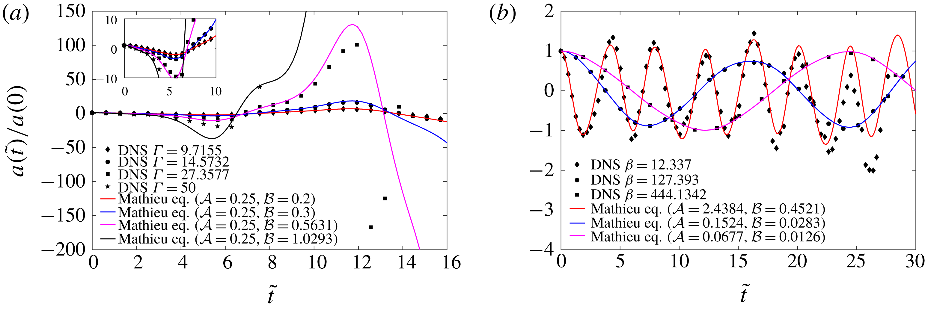
Figure 22. (a) Effect of changing
 $\unicode[STIX]{x1D6E4}$
. (b) Effect of changing
$\unicode[STIX]{x1D6E4}$
. (b) Effect of changing
 $\unicode[STIX]{x1D6FD}$
.
$\unicode[STIX]{x1D6FD}$
.
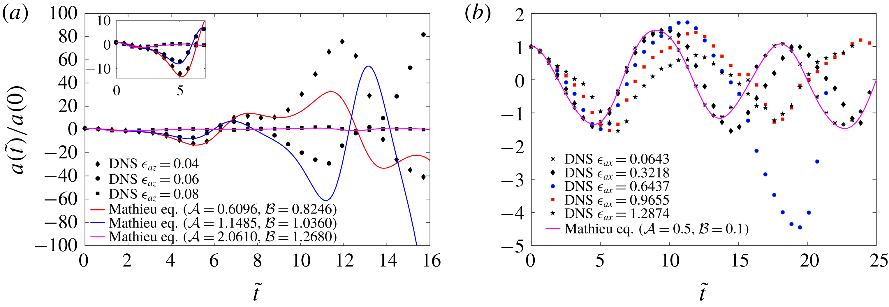
Figure 23. (a) Effect of changing
 $\unicode[STIX]{x1D716}_{az}$
. (b) Effect of changing
$\unicode[STIX]{x1D716}_{az}$
. (b) Effect of changing
 $\unicode[STIX]{x1D716}_{ax}$
.
$\unicode[STIX]{x1D716}_{ax}$
.
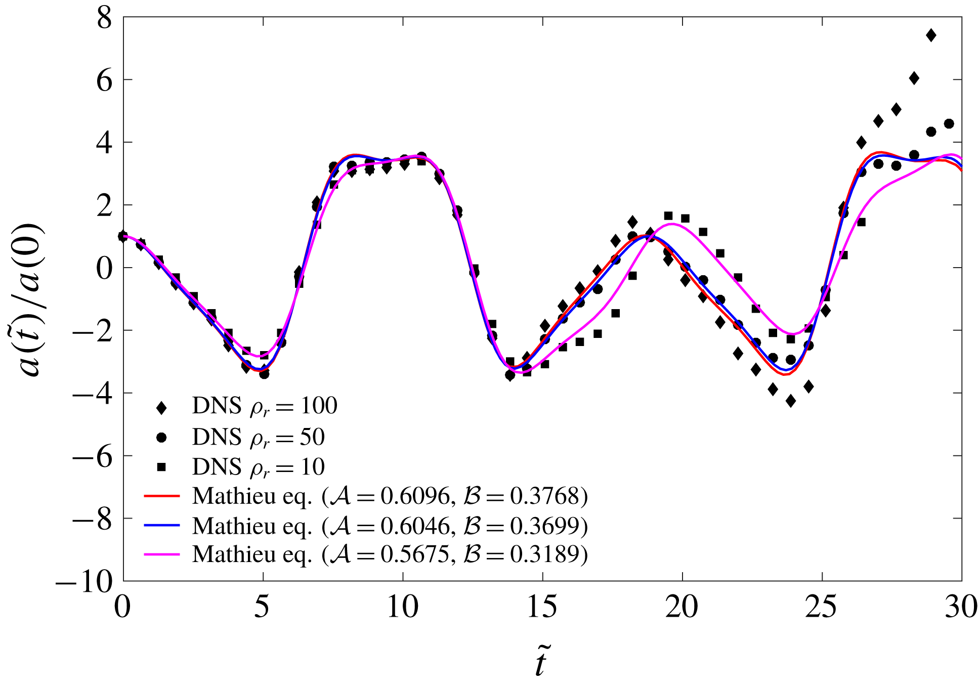
Figure 24. Effect of changing
 $\unicode[STIX]{x1D70C}_{r}$
.
$\unicode[STIX]{x1D70C}_{r}$
.
A systematic parametric study of the effect of changing the non-dimensional parameters
 $\unicode[STIX]{x1D6E4}$
,
$\unicode[STIX]{x1D6E4}$
,
 $\unicode[STIX]{x1D6FD}$
,
$\unicode[STIX]{x1D6FD}$
,
 $\unicode[STIX]{x1D716}_{az}$
,
$\unicode[STIX]{x1D716}_{az}$
,
 $\unicode[STIX]{x1D716}_{ax}$
and
$\unicode[STIX]{x1D716}_{ax}$
and
 $\unicode[STIX]{x1D70C}_{r}$
(see table 2) is reported in figures 22(a,b), 23(a,b) and 24, respectively. Figure 22(a) shows the effect of changing the non-dimensional forcing amplitude
$\unicode[STIX]{x1D70C}_{r}$
(see table 2) is reported in figures 22(a,b), 23(a,b) and 24, respectively. Figure 22(a) shows the effect of changing the non-dimensional forcing amplitude
 $\unicode[STIX]{x1D6E4}\equiv (\unicode[STIX]{x1D70C}^{{\mathcal{I}}}hR_{0}^{2}/T)$
(cases 11, 12, 13, 14 in table 2). Note that all the four simulations are linearly unstable and hence the amplitude grows with time (see stability chart
$\unicode[STIX]{x1D6E4}\equiv (\unicode[STIX]{x1D70C}^{{\mathcal{I}}}hR_{0}^{2}/T)$
(cases 11, 12, 13, 14 in table 2). Note that all the four simulations are linearly unstable and hence the amplitude grows with time (see stability chart
 $6b$
in supplementary material 1). It is seen that increasing
$6b$
in supplementary material 1). It is seen that increasing
 $\unicode[STIX]{x1D6E4}$
causes nonlinear effects to appear relatively early. In approximately two (non-dimensional) forcing time periods, i.e
$\unicode[STIX]{x1D6E4}$
causes nonlinear effects to appear relatively early. In approximately two (non-dimensional) forcing time periods, i.e
 $\tilde{t}=4\unicode[STIX]{x03C0}$
, significant deviation from the Mathieu solution is observed for case 13, while case 14 shows disintegration after
$\tilde{t}=4\unicode[STIX]{x03C0}$
, significant deviation from the Mathieu solution is observed for case 13, while case 14 shows disintegration after
 $\tilde{t}\approx 10$
. Within the same time window, case 11, which has the lowest value of
$\tilde{t}\approx 10$
. Within the same time window, case 11, which has the lowest value of
 $\unicode[STIX]{x1D6E4}$
, continues to show good agreement with the Mathieu solution. Figure 22(b) shows the effect of changing the non-dimensional forcing frequency
$\unicode[STIX]{x1D6E4}$
, continues to show good agreement with the Mathieu solution. Figure 22(b) shows the effect of changing the non-dimensional forcing frequency
 $\unicode[STIX]{x1D6FD}\equiv (\unicode[STIX]{x1D70C}^{{\mathcal{I}}}R_{0}^{3}\unicode[STIX]{x1D6FA}^{2}/T)$
(Cases 21, 22 and 23 in table 2, see stability charts
$\unicode[STIX]{x1D6FD}\equiv (\unicode[STIX]{x1D70C}^{{\mathcal{I}}}R_{0}^{3}\unicode[STIX]{x1D6FA}^{2}/T)$
(Cases 21, 22 and 23 in table 2, see stability charts
 $6i,6j$
and
$6i,6j$
and
 $6k$
in supplementary material 1). All the three simulations lie in the linearly stable regime. In dimensional time units, it is found that changing the forcing frequency by a factor of six causes very little change in the response frequency. Consequently, the three response curves in figure 22(b) plotted in non-dimensional time
$6k$
in supplementary material 1). All the three simulations lie in the linearly stable regime. In dimensional time units, it is found that changing the forcing frequency by a factor of six causes very little change in the response frequency. Consequently, the three response curves in figure 22(b) plotted in non-dimensional time
 $\tilde{t}\equiv \unicode[STIX]{x1D6FA}t$
are stretched out in proportion to their respective values of
$\tilde{t}\equiv \unicode[STIX]{x1D6FA}t$
are stretched out in proportion to their respective values of
 $\unicode[STIX]{x1D6FA}$
as seen in the figure, where the case for
$\unicode[STIX]{x1D6FA}$
as seen in the figure, where the case for
 $\unicode[STIX]{x1D6FD}=444.1342$
completes one oscillation when the case
$\unicode[STIX]{x1D6FD}=444.1342$
completes one oscillation when the case
 $\unicode[STIX]{x1D6FD}=12.337$
completes six oscillations (the value of
$\unicode[STIX]{x1D6FD}=12.337$
completes six oscillations (the value of
 $\unicode[STIX]{x1D6FA}$
for the former is six times that of the latter, as seen in table 2). Note that a change in forcing frequency also affects the amplitude of response, as seen in figure 22(b).
$\unicode[STIX]{x1D6FA}$
for the former is six times that of the latter, as seen in table 2). Note that a change in forcing frequency also affects the amplitude of response, as seen in figure 22(b).
In figure 23(a) we show the effect of changing
 $\unicode[STIX]{x1D716}_{az}\equiv (ma(0)/R_{0})$
. Due to the change in value of
$\unicode[STIX]{x1D716}_{az}\equiv (ma(0)/R_{0})$
. Due to the change in value of
 $m$
, case 17 becomes stable when compared to cases 15 and 16 in table 2. This is qualitatively similar to the RP instability, where introducing a non-zero azimuthal perturbation suppresses the instability. Both the unstable cases deviate from the Mathieu solution at approximately the same value of
$m$
, case 17 becomes stable when compared to cases 15 and 16 in table 2. This is qualitatively similar to the RP instability, where introducing a non-zero azimuthal perturbation suppresses the instability. Both the unstable cases deviate from the Mathieu solution at approximately the same value of
 $\tilde{t}\approx 8$
. Case 17, which is stabilised due to the higher value of
$\tilde{t}\approx 8$
. Case 17, which is stabilised due to the higher value of
 $m$
in the non-axisymmetric initial perturbation (see stability chart in figure 6(c–e) in supplementary material 1), displays a good agreement with DNS up to later times.
$m$
in the non-axisymmetric initial perturbation (see stability chart in figure 6(c–e) in supplementary material 1), displays a good agreement with DNS up to later times.
Figure 23(b) shows the effect of changing
 $\unicode[STIX]{x1D716}_{ax}\equiv a(0)k$
(Cases 5, 24, 25, 26 and 27 in table 2). These five simulations lie in the linearly stable regime and it is seen that the one with the smallest value of
$\unicode[STIX]{x1D716}_{ax}\equiv a(0)k$
(Cases 5, 24, 25, 26 and 27 in table 2). These five simulations lie in the linearly stable regime and it is seen that the one with the smallest value of
 $\unicode[STIX]{x1D716}_{ax}$
agrees with the linearised solution to the Mathieu equation for the longest time. It is clearly seen that for
$\unicode[STIX]{x1D716}_{ax}$
agrees with the linearised solution to the Mathieu equation for the longest time. It is clearly seen that for
 $\unicode[STIX]{x1D716}_{ax}>0.6437$
, the agreement with linear predictions is rather poor. Figure 24 shows the effect of changing the density ratio, where we have varied the density ratio by one order of magnitude (while restricting ourselves to
$\unicode[STIX]{x1D716}_{ax}>0.6437$
, the agreement with linear predictions is rather poor. Figure 24 shows the effect of changing the density ratio, where we have varied the density ratio by one order of magnitude (while restricting ourselves to
 $\unicode[STIX]{x1D70C}_{r}>1$
for this study). All three cases are in the linearly stable regime. It shows that a change of density ratio has only a small effect on the time of onset of nonlinearity. Linearised predictions from the Mathieu equation are seen to agree well over a change of an order of magnitude in the density ratio.
$\unicode[STIX]{x1D70C}_{r}>1$
for this study). All three cases are in the linearly stable regime. It shows that a change of density ratio has only a small effect on the time of onset of nonlinearity. Linearised predictions from the Mathieu equation are seen to agree well over a change of an order of magnitude in the density ratio.
6 Conclusions and future work
We have conducted a linear stability analysis of an interface separating two inviscid, immiscible, quiescent fluids subjected to a time-periodic body force. In a generalised curvilinear, orthogonal coordinate system where the Laplacian admits variable separable solutions, it is shown that the amplitude
 $a(t)$
of standing wave interfacial perturbations is governed by a generalised Mathieu equation. This equation unifies known results on Faraday waves in two geometries, viz. rectangular Cartesian (Benjamin & Ursell Reference Benjamin and Ursell1954) and spherical (Adou & Tuckerman Reference Adou and Tuckerman2016), and further shows that such waves can also be obtained on a cylindrical base state. Four classical dispersion relations are obtained, in the limit of zero forcing, from this equation. The principal novel findings of the study can be summarised as follows:
$a(t)$
of standing wave interfacial perturbations is governed by a generalised Mathieu equation. This equation unifies known results on Faraday waves in two geometries, viz. rectangular Cartesian (Benjamin & Ursell Reference Benjamin and Ursell1954) and spherical (Adou & Tuckerman Reference Adou and Tuckerman2016), and further shows that such waves can also be obtained on a cylindrical base state. Four classical dispersion relations are obtained, in the limit of zero forcing, from this equation. The principal novel findings of the study can be summarised as follows:
(1) A cylindrical capillary filament subject to a axisymmetric radial, time-periodic, body force is shown to be able to sustain Faraday waves and parametric instability.
(2) The amplitude of standing waves on the filament is governed by the Mathieu equation in the linearised limit. For small-amplitude perturbations and for small forcing amplitude, DNS results show very good agreement with the Mathieu solution.
(3) The stability chart of the Mathieu equation for the filament contains a special region (
 $m=0,kR_{0}<1$
) which is RP unstable in the absence of forcing. It is predicted that by choosing the forcing amplitude to lie in a certain range, RP modes can be stabilised.
$m=0,kR_{0}<1$
) which is RP unstable in the absence of forcing. It is predicted that by choosing the forcing amplitude to lie in a certain range, RP modes can be stabilised.(4) Stabilisation of RP modes via forcing is observed in DNS at early times. It is also seen that nonlinearity causes the emergence of higher wavenumbers, some of which are unstable due to forcing. These higher modes lead to eventual destabilisation of the filament. We show that this destabilisation can be understood from linear theory. Axisymmetric and 3D DNS are found to adopt different routes to instability.
(5) Similar to the suppression of RP instability using azimuthal perturbations, we show that unstable 3D Faraday waves can be stabilised by imposing perturbations of increasing azimuthal wavenumber.
(6) Parametric studies in a five-dimensional space of numbers clearly show the limits within which linearised theory yield accurate predictions. In particular, large values of
$\unicode[STIX]{x1D716}_{ax}$
and
$\unicode[STIX]{x1D6E4}$
are found to be associated with early onset of nonlinear effects.(7) Linearised theory is found to be unable to predict many interesting features which appear in DNS. Notably, in the unstable regime, depending on the symmetry of the initial perturbation, sheets and jets emerge from the cylindrical filament, suffering further instabilities and leading to fragmentation, pinch-off etc.


Certain lines of future study become clear. It is necessary to include the effect of viscosity in our analysis. Implications of this for damping of higher modes and prolonging the RP stabilisation requires detailed further study. A line of related enquiry is to extend the generalised equation, to include free and parametric oscillations of constrained interfaces with contact line or confinement constraints (see a recent review by Bostwick & Steen (Reference Bostwick and Steen2015)). It has been shown recently (Prosperetti Reference Prosperetti2012) that standard techniques used for analysing free oscillations can also be extended to such problems, leading to a simple harmonic oscillator equation with an integral term. The generalised Mathieu equation presented in this study should be extendable to these problems as well. We also note recent interesting results by Shen et al. (Reference Shen, Denner, Morgan, van Wachem and Dini2018), who study the effect of shear viscosity on capillary waves (in Cartesian geometry), demonstrating that the damped harmonic oscillator model of Denner (Reference Denner2016) predicts the critical wavelength (critically damped) to within two per cent of predictions from the complete viscous dispersion relation. In conclusion, we hope that the theoretical and numerical results presented here will motivate experiments on Faraday waves on a cylindrical filament.
Acknowledgements
We acknowledge an insightful suggestion from H. A. Stone which led us to derive a generalised, simple harmonic oscillator equation and thank him for correspondence and helpful comments. We acknowledge M. Singh for assistance with simulations and figures. We thank Science and Engineering Research Board (SERB, Dept. Science and Technology (DST), Govt. of India, # EMR/2016/000830) and the Industrial Research and Consultancy Centre (IRCC), IIT Bombay for PhD fellowship support and for funding a computational cluster.
Supplementary material and movies
Supplementary material and movies are available at https://doi.org/10.1017/jfm.2018.657.
Appendix A
We obtain an analytical approximation to the solution of (3.8) in the stable and unstable regimes for
 ${\mathcal{B}}\ll 1$
. When
${\mathcal{B}}\ll 1$
. When
 ${\mathcal{B}}=0$
, equation (3.8) is a simple harmonic oscillator equation with frequency
${\mathcal{B}}=0$
, equation (3.8) is a simple harmonic oscillator equation with frequency
 $\sqrt{{\mathcal{A}}}$
. For
$\sqrt{{\mathcal{A}}}$
. For
 ${\mathcal{B}}\ll 1$
, we obtain the solution using multiple scale analysis (Nayfeh Reference Nayfeh1973; Rand Reference Rand2016). A detailed derivation is provided in supplementary material 1. For
${\mathcal{B}}\ll 1$
, we obtain the solution using multiple scale analysis (Nayfeh Reference Nayfeh1973; Rand Reference Rand2016). A detailed derivation is provided in supplementary material 1. For
 ${\mathcal{A}}-n^{2}/4=O(1),n=1,2,3\ldots$
 $$\begin{eqnarray}\displaystyle \frac{a(t)}{r} & = & \displaystyle \cos \left[\unicode[STIX]{x1D711}t+\unicode[STIX]{x1D6E9}\right]+\frac{{\mathcal{B}}}{2\sqrt{{\mathcal{A}}}+1}\cos \left[\left(\unicode[STIX]{x1D711}+1\right)t+\unicode[STIX]{x1D6E9}\right]-\frac{{\mathcal{B}}}{2\sqrt{{\mathcal{A}}}-1}\cos \left[\left(\unicode[STIX]{x1D711}-1\right)t+\unicode[STIX]{x1D6E9}\right]\nonumber\\ \displaystyle & & \displaystyle +\,\frac{{\mathcal{B}}^{2}}{4(\sqrt{{\mathcal{A}}}+1)(2\sqrt{{\mathcal{A}}}+1)}\cos \left[\left(\unicode[STIX]{x1D711}+2\right)t+\unicode[STIX]{x1D6E9}\right]\nonumber\\ \displaystyle & & \displaystyle +\,\frac{{\mathcal{B}}^{2}}{4(\sqrt{{\mathcal{A}}}-1)(2\sqrt{{\mathcal{A}}}-1)}\cos \left[\left(\unicode[STIX]{x1D711}-2\right)t+\unicode[STIX]{x1D6E9}\right]+O({\mathcal{B}}^{3}),\end{eqnarray}$$
where
 $\unicode[STIX]{x1D711}\equiv \sqrt{{\mathcal{A}}}-(B^{2}/\sqrt{{\mathcal{A}}}(4{\mathcal{A}}-1))$
and
$\unicode[STIX]{x1D711}\equiv \sqrt{{\mathcal{A}}}-(B^{2}/\sqrt{{\mathcal{A}}}(4{\mathcal{A}}-1))$
and
 $r$
and
$r$
and
 $\unicode[STIX]{x1D6E9}$
are constants determined from initial conditions. Similarly in the first unstable tongue labelled
$\unicode[STIX]{x1D6E9}$
are constants determined from initial conditions. Similarly in the first unstable tongue labelled
 $SH$
in the inset of figure 4, this solution to
$SH$
in the inset of figure 4, this solution to
 $O({\mathcal{B}})$
is
$O({\mathcal{B}})$
is
 $$\begin{eqnarray}\displaystyle a(t) & = & \displaystyle 2K_{1}\exp ({\mathcal{B}}t\sqrt{1-{\mathcal{A}}_{1}^{2}})\left(\sqrt{\frac{1-{\mathcal{A}}_{1}}{1+{\mathcal{A}}_{1}}}\cos \left(t/2\right)-\sin \left(t/2\right)\right)\nonumber\\ \displaystyle & & \displaystyle -\,2K_{2}\exp (-{\mathcal{B}}t\sqrt{1-{\mathcal{A}}_{1}^{2}})\left(\sqrt{\frac{1-{\mathcal{A}}_{1}}{1+{\mathcal{A}}_{1}}}\cos \left(t/2\right)+\sin \left(t/2\right)\right)\nonumber\\ \displaystyle & & \displaystyle +\,{\mathcal{B}}K_{1}\exp ({\mathcal{B}}t\sqrt{1-{\mathcal{A}}_{1}^{2}})\left(\sqrt{\frac{1-{\mathcal{A}}_{1}}{1+{\mathcal{A}}_{1}}}\cos \left(3t/2\right)-\sin \left(3t/2\right)\right)\nonumber\\ \displaystyle & & \displaystyle -\,{\mathcal{B}}K_{2}\exp (-{\mathcal{B}}t\sqrt{1-{\mathcal{A}}_{1}^{2}})\left(\sqrt{\frac{1-{\mathcal{A}}_{1}}{1+{\mathcal{A}}_{1}}}\cos \left(3t/2\right)+\sin \left(3t/2\right)\right)\nonumber\\ \displaystyle & & \displaystyle +\,O({\mathcal{B}}^{2}),\end{eqnarray}$$
where
 $K_{1}$
and
$K_{1}$
and
 $K_{2}$
are constants to be determined from initial conditions. Expression (A 2) shows that, for
$K_{2}$
are constants to be determined from initial conditions. Expression (A 2) shows that, for
 $-1<{\mathcal{A}}_{1}<1$
, we have exponentially growing solutions. Expressions (A 1) and (A 2) are used for comparison with our DNS results in § 5.
$-1<{\mathcal{A}}_{1}<1$
, we have exponentially growing solutions. Expressions (A 1) and (A 2) are used for comparison with our DNS results in § 5.