


INTRODUCTION
The terminal Pleistocene (20,000–11,700 cal yr BP) encompassed a period of substantial restructuring of North American terrestrial ecosystems, which were linked to the combined effects of changing climate and substantial biodiversity loss (e.g., Barnosky et al., Reference Barnosky, Lindsey, Villavicencio, Bostelmann, Hadly, Wanket and Marshall2016; Cotton et al., Reference Cotton, Cerling, Hoppe, Mosier and Still2016; Smith et al., Reference Smith, Tomé, Elliott Smith, Lyons, Newsome and Stafford2016b; Tóth et al., Reference Tóth, Lyons, Barr, Behrensmeyer, Blois, Bobe and Matt Davis2019). As glaciers retreated to the north after the last glacial maximum at 21,000 cal yr BP, climate warmed by ~8°C overall, although this warming was interrupted by numerous temperature reversals (Cole and Arundel, Reference Cole and Arundel2005; IPCC, 2014). The most notable of these was the Younger Dryas (12,800–11,500 cal yr BP), a 1,300 year period of cooling to near glacial conditions, which ended in a particularly rapid 5–7°C increase in temperature over a few decades (Dansgaard, Reference Dansgaard, White and Johnsen1989; Alley, Reference Alley2000). These environmental fluctuations influenced the composition and distribution of flora and fauna across North America (Prentice et al., Reference Prentice, Bartlein and Webb1991; Graham et al., Reference Graham, Lundelius, Graham, Schroeder, Toomey, Anderson and Barnosky1996; Grayson, Reference Grayson2000; Lyons, Reference Lyons2003, Reference Lyons2005; Blois et al., Reference Blois, McGuire and Hadly2010; Cotton et al., Reference Cotton, Cerling, Hoppe, Mosier and Still2016).
The terminal Pleistocene was also unique because within a few hundred years, virtually all large-bodied mammals (>150 species) went extinct in the Americas (Martin, Reference Martin, Martin and Wright1967; Martin and Klein, Reference Martin and Klein1989; Martin and Steadman, Reference Martin, Steadman and MacPhee1999; Lyons et al., Reference Lyons, Smith and Brown2004). Highly size-selective, this event saw the loss of all mammals weighing >600 kg—a diverse group of megafauna including mammoths, camels, and giant ground sloths (Lyons et al., Reference Lyons, Smith and Brown2004; Smith et al., Reference Smith, Elliott Smith, Lyons and Payne2018). Large-bodied mammals have substantial impacts within modern communities and ecosystems, both through environmental engineering and species interactions (Janzen and Martin, Reference Janzen and Martin1982; Owen-Smith, Reference Owen-Smith1992; Ripple et al., Reference Ripple, Newsome, Wolf, Dirzo, Everatt, Galetti and Hayward2015; Malhi et al., Reference Malhi, Doughty, Galetti, Smith, Svenning and Terborgh2016; Smith et al., Reference Smith, Doughty, Malhi, Svenning and Terborgh2016a). For example, extant megaherbivores in Africa help maintain savanna and grassland habitats by suppressing woody growth, modifying fire regimes, and acting as seed dispersers for plants (Dublin et al., Reference Dublin, Sinclair and McGlade1990; Owen-Smith, Reference Owen-Smith1992; Goheen et al., Reference Goheen, Palmer, Keesing, Riginos and Young2010, Reference Goheen, Augustine, Veblen, Kimuyu, Palmer, Porensky and Pringle2018). Exclusion of these large-bodied mammals can result in shifts in vegetation composition and abundance and/or alter the distribution and abundance of other mammals, such as rodents, via competitive interactions (Keesing, Reference Keesing1998; Goheen et al., Reference Goheen, Keesing, Allan, Ogada and Ostfeld2004, Reference Goheen, Augustine, Veblen, Kimuyu, Palmer, Porensky and Pringle2018; Parsons et al., Reference Parsons, Maron and Martin2013; Keesing and Young, Reference Keesing and Young2014; Koerner et al., Reference Koerner, Burkepile, Flynn, Burns, Eby, Govender and Hagenah2014; Galetti et al., Reference Galetti, Guevara, Neves, Rodarte, Bovendorp, Moreira, Hopkins and Yeakel2015). Pleistocene megafauna are thought to have played roles similar to their modern counterparts by maintaining open habitats and enhancing species diversity, repressing fire regimes, and increasing nutrient availability across ecosystems (Johnson, Reference Johnson2009; Rule et al., Reference Rule, Brook, Haberle, Turney, Kershaw and Johnson2012; Doughty et al., Reference Doughty, Wolf and Malhi2013; Ripple et al., Reference Ripple, Newsome, Wolf, Dirzo, Everatt, Galetti and Hayward2015; Bakker et al., Reference Bakker, Gill, Johnson, Vera, Sandom, Asner and Svenning2016). In addition to structural changes in vegetation, the extinction likely had cascading effects on community structure and interactions of the surviving mammal species (Smith et al., Reference Smith, Tomé, Elliott Smith, Lyons, Newsome and Stafford2016b; Tóth et al., Reference Tóth, Lyons, Barr, Behrensmeyer, Blois, Bobe and Matt Davis2019).
How these wholesale changes in community dynamics and climate influenced surviving species likely depended on whether species were more sensitive to abiotic or biotic interactions. Changes in temperature often lead to shifts in body size, diet, or both, either as a direct consequence of thermal physiology or due to shifting vegetation composition (Bergmann, Reference Bergmann1847; Brown, Reference Brown1968; Andrewartha and Birch, Reference Andrewartha and Birch1986; Brown and Heske, Reference Brown and Heske1990; Smith et al., Reference Smith, Betancourt and Brown1995; Ashton et al., Reference Ashton, Tracy and Queiroz2000; Stenseth et al., Reference Stenseth, Mysterud, Ottersen, Hurrell, Chan and Lima2002; Millien et al., Reference Millien, Lyons, Olson, Smith, Wilson and Yom-Tov2006; Walsh et al., Reference Walsh, Aprigio Assis, Patton, Marroig, Dawson and Lacey2016). Because body size scales with most life history traits and physiological processes, including metabolism, ingestion, and thermal regulation (McNab, Reference McNab1980; Peters, Reference Peters1983; Justice and Smith, Reference Justice and Smith1992; Smith, Reference Smith1995a), size can influence the types and amounts of resources available to consumers, as well as inter- and intraspecies interactions among consumers (Damuth, Reference Damuth1981; Peters, Reference Peters1983). At a local scale, enhanced competition for habitat and resources will decrease the abundances of species of similar size that share resources (Brown, Reference Brown1973; M'Closkey, Reference M'Closkey1976; Bowers and Brown, Reference Bowers and Brown1982; Brown and Nicoletto, Reference Brown and Nicoletto1991; Auffray et al., Reference Auffray, Renaud and Claude2009). The relationship between body size and other ecological factors (such as home range or competition), particularly when combined with dietary and environmental information, can be used to quantify complex ecosystem and community changes recorded in the paleontological record (Damuth, Reference Damuth1981).
Here, we characterize the response of Neotoma (woodrats) to environmental and ecological perturbations on the Edwards Plateau (Texas) (Fig. 1A–B) over the past ca. 22,000 years. We quantify shifts in body size and diet using digital imaging of fossil molars and stable isotope analysis of associated bone collagen, respectively. We focus on a complex of three potential Neotoma species—N. albigula (white-throated woodrat), N. floridana (eastern woodrat), and N. micropus (southern plains woodrat)—which differ in body size, dietary preferences, and habitat affinity. All species of Neotoma are herbivorous and construct large dens. Neotoma albigula (~155–250 g) and N. micropus (~180–320 g) both inhabit desert and semi-arid environments and are reliant on cacti for den construction and as a source of food and water (Olsen, Reference Olsen1976; Macêdo and Mares, Reference Macêdo and Mares1988; Braun and Mares, Reference Braun and Mares1989; Orr et al., Reference Orr, Newsome and Wolf2015). In contrast, N. floridana (~200–380 g) typically inhabit more mesic, forested environments, do not usually forage on cacti, and typically eat higher proportions of leaves and fruit from trees and shrubs (Rainey, Reference Rainey1956; Finley, Reference Finley1958; Wiley, Reference Wiley1980). Woodrat dens are typically built within rock crevices, which provide protection from both predators and extreme temperatures (Finley, Reference Finley1958; Brown, Reference Brown1968; Brown et al., Reference Brown, Lieberman and Dengler1972; Smith, Reference Smith1995b; Murray and Smith, Reference Murray and Smith2012). Past studies of Neotoma suggest all species within the genus are highly sensitive to temperature; morphological changes in size are a common response to temperature fluctuations across both space and time (Brown and Lee, Reference Brown and Lee1969; Smith et al., Reference Smith, Betancourt and Brown1995, Reference Smith, Browning and Shepherd1998; Smith and Betancourt, Reference Smith and Betancourt1998, Reference Smith and Betancourt2003). These changes in size align with the ecological principle known as Bergmann's Rule—the idea that within a genus, those species inhabiting colder environments will be larger than those in warmer ones (Bergmann, Reference Bergmann1847; Mayr, Reference Mayr1956; Brown and Lee, Reference Brown and Lee1969; Ashton et al., Reference Ashton, Tracy and Queiroz2000; Freckleton et al., Reference Freckleton, Harvey and Pagel2003; Smith, Reference Smith, Jorgensen and Fath2008). Thus, we hypothesize that Neotoma species were strongly influenced by temperature fluctuations on the Edwards Plateau, with increasing Holocene temperatures leading to a decrease in body mass.
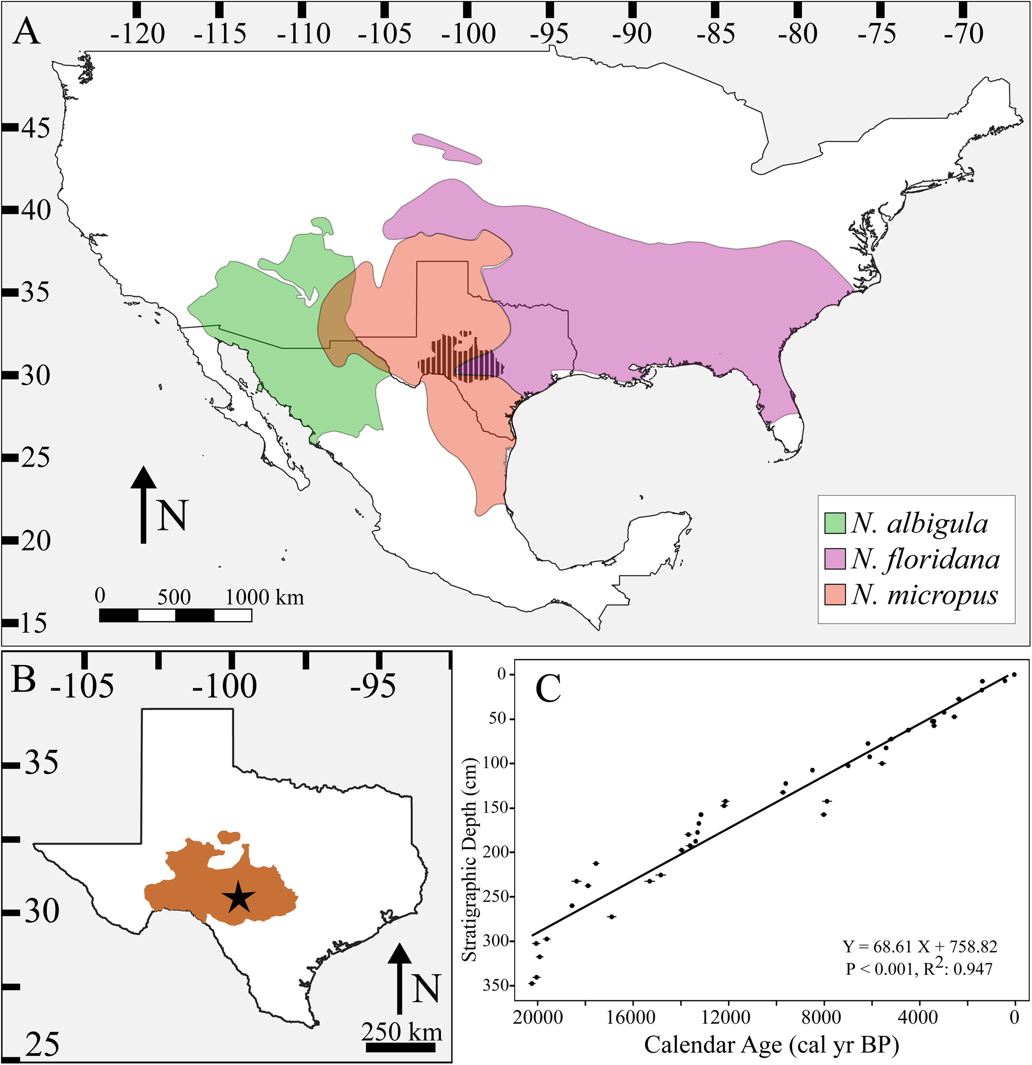
Figure 1. Neotoma species distributions. (A) Map of North America with modern distributions of Neotoma albigula (green), N. floridana (purple), and N. micropus (red). Location of the Edwards Plateau in Texas is represented by cross-hatched black area. (B) Map of Texas with Edwards Plateau highlighted in brown and location of Hall's Cave (star). (C) The age model, which is composed of 44 AMS 14C measurements previously combined from Toomey (Reference Toomey1993), Cooke et al. (Reference Cooke, Stern, Banner, Mack, Stafford and Toomey III2003), and Bourne et al. (Reference Bourne, Feinberg, Stafford, Waters, Lundelius and Forman2016) and calibrated by Tomé et al. (Reference Tomé, Elliott Smith, Lyons, Newsome and Smith2020a).
Changes in vegetation associated with climate and the terminal Pleistocene megafaunal extinction may have also led to shifts in resource availability and competition among consumers that are reflected in shifts in diet composition among sympatric species. Body mass is an important component of interspecific interactions for Neotoma. When different species of Neotoma occur in sympatry, the smaller-bodied species may shift microhabitats or diet to partition resources with larger-bodied ones (Finley, Reference Finley1958; Cameron, Reference Cameron1971; Dial, Reference Dial1988). For example, where they co-occur with larger N. fuscipes (~230–300 g), N. lepida (~120–240 g) switch from feeding on oaks (Quercus turbinella) to feeding on juniper (Juniperus californica); consumption of juniper has a higher metabolic and thermoregulatory cost for woodrats because it contains higher concentrations of toxic secondary compounds (Cameron, Reference Cameron1971; Carraway and Verts, Reference Carraway and Verts1991; Verts and Carraway, Reference Verts and Carraway2002; McLister et al., Reference McLister, Sorensen and Dearing2004; Dearing et al., Reference Dearing, McLister and Sorensen2005). Community reorganization following the extinction thus may have influenced dietary responses in Neotoma either though changes in competition for available resources or through shifts in the relative abundance of vegetation driven by the absence of megaherbivores.
We assessed dietary changes over time with carbon (δ13C) and nitrogen (δ15N) isotope analyses of bone collagen, which have previously been used to quantify changes in diet composition, trophic level, and niche partitioning across space and time (Chamberlain et al., Reference Chamberlain, Waldbauer, Fox-Dobbs, Newsome, Koch, Smith and Church2005; West et al., Reference West, Bowen, Cerling and Ehleringer2006; Koch et al., Reference Koch, Fox-Dobbs, Newsome, Dietl and Flessa2009; Leonard et al., Reference Leonard, Vilà, Fox-Dobbs, Koch, Wayne and Van Valkenburgh2007; Smiley et al., Reference Smiley, Cotton, Badgley and Cerling2016). Changes in diet and body size may also reflect species preferences in terms of environmental conditions and resource availability. During the last glacial maximum (ca. 21,000 cal yr BP), the Edwards Plateau was a mix of deciduous forest and conifers, before warming and drying conditions during the late-glacial period (17,000–11,600 cal yr BP) led to the transition to a grassland and oak savanna landscape (Bryant and Holloway, Reference Bryant, Holloway, Bryant and Holloway1985; Cordova and Johnson, Reference Cordova and Johnson2019). This vegetation remained relatively stable throughout the Holocene (11,600–0 cal yr BP), and today the region is predominantly a savanna shrub woodland populated by oak, mesquite, and juniper (Bryant and Holloway, Reference Bryant, Holloway, Bryant and Holloway1985; Toomey et al., Reference Toomey, Blum and Valastro1993; Joines, Reference Joines2011). As regional vegetation shifted from mesic conditions preferred by N. floridana to a drier shrubland more preferred by N. albigula and N. micropus, we may expect to see shifts in diet towards resources more typically used by arid-adapted woodrats (e.g., higher consumption of cacti) due either to changes in resource use or changes in the relative abundance of these three species over time.
METHODS
Study site
We used fossils from Hall's Cave in the Edwards Plateau, Texas (Fig. 1B). This site is a fluvial deposit with episodic deposition of sediments and biological materials following heightened periods of precipitation (Toomey, Reference Toomey1993). The Hall's Cave record extends back to ca. 20,000 cal yr BP, with an exceptionally well-dated stratigraphic sequence (Fig. 1C). Excavations from Hall's Cave began in the 1960s and accelerated in the late 1980s–1990s (Toomey, Reference Toomey1993). To date, the site has yielded thousands of vertebrate specimens, particularly of small and medium body sizes across various trophic guilds (Toomey, Reference Toomey1993). The vertebrate fossils are housed at the Vertebrate Paleontology Lab of the Texas Memorial Museum (TMM) at the University of Texas, Austin.
Study organisms
Three Neotoma species are hypothesized to be present in the Hall's Cave fossil record: N. albigula, N. floridana, and N. micropus (Toomey, Reference Toomey1993), with the latter two extant on the Edward's Plateau today (Fig. 1A). Unfortunately, the three species cannot be distinguished based solely on molar or lower-jaw characteristics (Sagebiel, Reference Sagebiel2010; Tomé et al., Reference Tomé, Whiteman-Jennings and Smith2020b), which represent the vast majority of our fossil elements. Moreover, there is substantial body size overlap among the species. Thus, we aggregated samples and asked questions at the level of the genus, which we note is common for paleoecological studies. Nonetheless, we note that preliminary ancient DNA work conducted on a sediment column taken from Hall's Cave suggested a high probability that Neotoma floridana is the only woodrat present in the oldest (prior to the extinction boundary at ca. 13,000 cal yr BP) stratigraphic levels (Seersholm et al., Reference Seersholm, Werndly, Grealy, Johnson, Keenan Early, Lundelius and Winsborough2020).
Neotoma fossils are present in all strata at Hall's Cave from ca. 22,000 cal yr BP to modern deposits (Toomey, Reference Toomey1993); however, specimen abundance varies by stratum. To facilitate our analyses of body size and diet of Neotoma over time, we aggregated data into 15 time intervals of approximately equal length, chosen and accounting for important environmental transitions (Table 1). Note that the oldest time interval is longer, spanning 22,400–15,800 cal yr BP; this is because Neotoma fossil bones were rare, with only 31 elements recovered in this interval. Thus, to increase sample size, we also included a sample of 14 additional Neotoma specimens from Zesch Cave, a nearby fossil site, ~75 km away, at 470 m in elevation, and dating to 18,000–16,000 cal yr BP (Lundelius, Reference Lundelius, Martin and Wright1967; Graham et al., Reference Graham, Graham, Semken and Graham1987; Sagebiel, Reference Sagebiel2010). The Zesch Cave record shares a similar community composition to that of Hall's Cave, including the same three potential Neotoma species. To verify that climatic regimes at this time were similar between Zesch Cave and Hall's Cave (~680 m elevation), we compared climate data from the Community Climate System Model (Lorenz et al., Reference Lorenz, Nieto-Lugilde, Blois, Fitzpatrick and Williams2016a, Reference Lorenz, Nieto-Lugilde, Blois, Fitzpatrick and Williamsb). We found that mean annual precipitation, maximum temperature, and minimum temperature differed by ~32.5 mm, ~7.1°C, and 4.7°C, respectively, between the two sites, with temperature differences falling within one standard deviation for the time bin spanning 22,400–15,800 cal yr BP. Two sample t-tests found no significant difference in body size or bone collagen δ13C and δ15N values of Neotoma from Zesch Cave and Hall's Cave (Supplementary Table S1). All other (i.e., younger) time bins include only specimens from Hall's Cave.
Table 1. Summary of data for Neotoma by time interval. Precipitation, maximum and minimum temperature were extracted from the CCM3 (Lorenz et al., Reference Lorenz, Nieto-Lugilde, Blois, Fitzpatrick and Williams2016a, Reference Lorenz, Nieto-Lugilde, Blois, Fitzpatrick and Williamsb) in 500 year intervals and average each time interval given below. Sorenson to Modern is the Sorenson Index calculated in terms of similarity to the community composition of the youngest time interval (0–1500 cal BP).

Morphology
We estimated body size in Neotoma using linear measurements of the first upper (UM1) and lower molars (LM1). These molars were either loose or found in mandibular or maxillary elements, generally with incomplete toothrows. The upper or lower M1 of 693 Neotoma fossils were photographed using a calibrated AM4515ZT Dino-Lite Edge digital microscope. The length of each molar was measured three times (~2080 measurements) using the line tool in DinoCapture 2.0. Samples that could not be well characterized or whose measurements resulted in a >5% standard error were discarded, which led to the elimination of 22 specimens. We calculated the minimum number of individuals (MNI) to exclude potentially replicated individuals because it was not possible to determine whether loose molars were definitively from different specimens or potentially from different quadrants (upper right and left, and lower right and left) from the same individual.
To help in the estimation of MNI, we determined the ‘normal’ asymmetry of teeth found among modern woodrats. By measuring all the first molars (upper and lower, right and left) for a total of 20 museum specimens, which included individuals from the species Neotoma floridana and N. albigula from the Museum of Southwestern Biology (MSB) at the University of New Mexico (Albuquerque, NM) and the James F. Bell Museum of Natural History (MMNH) at the University of Minnesota (St. Paul, MN) (Supplementary Table S2), we characterized the upper versus lower and bilateral symmetry of woodrat teeth. We found that on average, upper first molars (UM1) were ~5% larger than lower first molars (LM1). Moreover, bilateral symmetry was high, with only an average difference of ~0.5% between left and right measurements. These results were independent of species and provided a strategy for analysis: using 0.5% as a cutoff we were able to determine whether loose molars from a stratum could realistically belong to different Neotoma. First, we preferentially selected only lower left first molars (LLM1s) for each stratigraphic level. Second, we then included all lower right first molars (LRM1s) from that level that were 0.5% greater or smaller in size than any measured LLM1s in the sample. Third, after standardizing the size of upper molars to that of lower molars with a 5% length reduction, we included upper left first molars (ULM1s) from that level that were 0.5% greater or smaller in size than any lower molars selected in the first two steps. Lastly, we included upper right first molars (URM1s) from the same level that were 0.5% greater or smaller in size than any previously selected LLM1s, LRM1s, and ULM1s. Thus, we ensured that separately measured elements were not from the same individual within a stratum.
Tooth measurements were translated into estimates of body mass using an allometric equation for cricetid rodents for the first lower molar length (Martin, Reference Martin, Damuth and MacFadden1990):

To account for differences between lower and upper molar length in Neotoma, upper molar length was standardized by a 5% decrease to measurements prior to calculating body mass. After the removal of potential duplicates, our final dataset included body mass estimates for 430 individual Neotoma across the 15 levels, including mass estimates for 10–63 individuals per time bin (Table 1).
Isotope-based estimates of diet composition and variation
We used stable isotope analysis to characterize shifts in diet for Neotoma across time. We measured carbon (δ13C) and nitrogen (δ15N) isotope values of bone collagen extracted from maxillary and mandible bones for 367 Neotoma fossils. We attempted to acquire 10 or more samples per time interval; however, sparsity of material led to some intervals containing fewer than 10 individuals, and we excluded a single interval that only contained five individuals (22,400–15,800 cal yr BP). Differences in how plants that use the C3 versus C4 photosynthetic pathway fractionate carbon isotopes leads to natural variation in δ13C values across ecosystems and are reflected in the tissues of consumers that utilize these resources (DeNiro and Epstein, Reference DeNiro and Epstein1978; Farquhar et al., Reference Farquhar, Ehleringer and Hubick1989; Cerling et al., Reference Cerling, Harris, MacFadden, Leakey, Quade, Eisenmann and Ehleringer1997). Regional studies in the Great Plains and southern/central Texas have found that C3 and C4 plants have mean (±SD) δ13C values of about -27 ± 5‰ and -13 ± 4‰, respectively (Boutton et al., Reference Boutton, Nordt, Archer, Midwood and Casar1993, Reference Boutton, Archer, Midwood, Zitzer and Bol1998; Derner et al., Reference Derner, Boutton and Briske2006). δ15N values of consumers reflect a combination of trophic position and/or shifts in the baseline nitrogen isotope composition of primary producers, with higher δ15N values signifying higher trophic position or increased aridity (DeNiro and Epstein, Reference DeNiro and Epstein1981; Ambrose, Reference Ambrose1991; Amundson et al., Reference Amundson, Austin, Schuur, Yoo, Matzek, Kendall, Uebersax, Brenner and Baisden2003). Consumer tissue δ13C and δ15N values systematically differ from that of their diet due to physiologically mediated isotopic discrimination (Koch, Reference Koch, Michener and Lajtha2007) and these differences are quantified as trophic discrimination factors (TDF). Thus, at a particular time interval, δ13C and δ15N values vary across animals in a community depending upon their trophic level and the relative proportion of C3 versus C4 vegetation in their diet, which allows for use of isotopic niche space of small mammals that do not move large distance as a proxy for dietary niche space (Newsome et al., Reference Newsome, Martinez del Rio, Bearhop and Phillips2007).
A subsample of ~150–250 mg of bone was collected from each fossil mandible or maxilla using a low-speed Dremel tool. To extract collagen, we demineralized samples with 0.25N HCl at 3–4°C for 24–48 hours. Samples were then lipid extracted via soaking in 2:1 chloroform/methanol for 72 hours, changing the solution every 24 hours. Each sample was then washed 5–7 times with distilled water and lyophilized. Approximately 0.9–1.0 mg of collagen was placed into 3 × 5 mm tin capsules. Collagen δ13C and δ15N values were measured with a Costech elemental analyzer (Valencia, CA) interfaced with a Thermo Scientific Delta V Plus isotope ratio mass spectrometer (Bremen, Germany) at the University of New Mexico Center for Stable Isotopes (Albuquerque, NM). Isotope values are reported as δ values, where δ = 1000[(Rsample/Rstandard)-1] and Rsamp and Rstd are the 13C:12C or 15N:14N ratios of the sample and standard, respectively; units are in parts per thousand, or per mil (‰). Samples were calibrated using international reference standards; Vienna Pee Dee Belemnite (VPDB) for carbon, and atmospheric N2 for nitrogen (Fry, Reference Fry2006; Sharp, Reference Sharp2017). Analytical precision was assessed via repeated within-run analysis of organic reference materials calibrated to international standards and was determined as ≤0.2‰ for both δ13C and δ15N values. We also measured the weight percent carbon and nitrogen concentration of each collagen sample. Mean (±SD) [C]:[N] ratios for Neotoma (N = 378) were 2.9 ± 0.14 and we excluded any samples from subsequent analyses whose [C]:[N] ratios were >3.5 (Ambrose, Reference Ambrose1990).
We followed our protocol for MNI as outlined above for the mass estimates to ensure that each sample chosen for isotope analysis represented a unique individual. Our final dataset for the isotopic analyses consisted of 306 individuals (Table 1). Not all specimens for which we had δ13C and δ15N measurements had body measurements, and vice versa. Of the 430 individuals with mass measurements and 306 with isotope measurements, 131 individuals had both.
Community, climate, and vegetation data
We compared our body-size and isotope data with measures of the mammal community composition and turnover, climate (temperature and precipitation), and several measures of vegetation composition and change. Community data included α-diversity (richness) and β-diversity (Sorenson Index) extracted from Smith et al. (Reference Smith, Tomé, Elliott Smith, Lyons, Newsome and Stafford2016b), updated to reflect current phylogeny and cave fossil assembly information, and recalculated to fit within the time intervals used here (Table 1). Here, we used the Sorenson Index to calculate turnover between adjacent time intervals and similarity to the modern community composition. Turnover, defined as similarity to the previous time interval, can be used to evaluate changes in species composition between time bins and provides information on whether the presence/absence of certain species may be affecting responses in Neotoma. Similarity to modern provides insight into whether species turnover is related to species permanently leaving the community and being replaced or leaving and re-entering the community through time. The original community data for Hall's Cave were compiled by Toomey (Reference Toomey1993) and expanded to encompass the Edwards Plateau using the Neotoma Paleoecology Database (2015) by Smith et al. (Reference Smith, Tomé, Elliott Smith, Lyons, Newsome and Stafford2016b).
Climate information was sourced from the Community Climate System Model (CCSM3), which simulates climate across North America for the past 21,000 years (Lorenz et al., Reference Lorenz, Nieto-Lugilde, Blois, Fitzpatrick and Williams2016a, Reference Lorenz, Nieto-Lugilde, Blois, Fitzpatrick and Williamsb). The CCSM3 data have 0.5° spatial resolution, so we were able to obtain regional-scale climate for the Edwards Plateau. Mean annual maximum and minimum temperature and total mean annual precipitation data were extracted from the CCSM3 at 500 year intervals. We averaged values to the same temporal intervals used for our fossil morphometric and isotopic data (Table 1; Fig. 2A–C).

Figure 2. Temporal changes in climate and vegetation on the Edwards Plateau, including (A) mean maximum temperature, (B) mean minimum temperature, and (C) mean annual precipitation (mm) (Lorenz et al., Reference Lorenz, Nieto-Lugilde, Blois, Fitzpatrick and Williams2016a, Reference Lorenz, Nieto-Lugilde, Blois, Fitzpatrick and Williamsb). (D) Pollen counts showing the relative abundance of C3 versus C4 (%) grasses (C3 grasses/C4 grasses × 100), Cupressaceae, and Opuntia at Hall's Cave over time (Cordova and Johnson Reference Cordova and Johnson2019).
We compared the Neotoma body-size and isotope data with a vegetation reconstruction from Hall's Cave based on phytolith and pollen data from 47 stratigraphic depths spanning the past 18,000 years (Cordova and Johnson, Reference Cordova and Johnson2019). The ratio of C3 to C4 grasses derived from phytolith data serves as an index for the prevalence of C4 grasses on the landscape, with declining C3:C4 values during the Holocene reflecting a shift from forests dominated by C3 plants to grasslands dominated by C4 grasses in response to drier conditions (Cordova and Johnson, Reference Cordova and Johnson2019). Because modern Neotoma albigula, N. floridana, and N. micropus differ in their use of prickly pear cacti and juniper, we also compared our Neotoma data with changes in the relative abundance of Opuntia (prickly pear) and Cupressaceae (the family including juniper) pollen. Modern Neotoma albigula and N. micropus are known to consume prickly pear cacti, which can represent up to 45% of the annual diet of N. albigula (Vorhies and Taylor, Reference Vorhies and Taylor1940; Spencer and Spencer, Reference Spencer and Spencer1941; Macêdo and Mares, Reference Macêdo and Mares1988; Braun and Mares, Reference Braun and Mares1989). Moreover, N. albigula makes more use of juniper than either Neotoma floridana or Neotoma micropus (Rainey, Reference Rainey1956; Finley, Reference Finley1958; Wiley, Reference Wiley1980; Dial, Reference Dial1988; Schmidly and Bradley, Reference Schmidly and Bradley2016). We calculated mean values of C3:C4 grasses in the phytolith data and mean pollen percentages for Opuntia and Cupressaceae for each of our 15 time intervals (Fig. 2D).
Statistical analyses
We employed both parametric and non-parametric tests to examine changes in body mass and isotope values over time because in some instances our data violated assumptions of normality. All statistical analyses were performed using R software version R.3.6.0 (R Core Team, 2019) and RStudio 1.2.1335 (RStudio Team, 2019).
We first used an F-test and a Bartlett's test to assess changes in body mass and isotope variation before and after the extinction boundary (ca. 13,000 cal yr BP) to determine if there were marked changes associated with this period of acute biodiversity loss. To examine changes in mass across all 15 time intervals, we used ANOVA and Tukey multiple comparisons. Least squares linear regressions were also run using maximum (i.e., largest individual per time interval) and median mass against the mean δ13C, δ15N, climate, and community variables to evaluate their influence on body mass. When significant correlations were found, we conducted an analysis of covariance (ANCOVA) to assess the added effect of each on mass.
We characterized shifts in isotopic niche space using Bayesian-based standard ellipse areas (SEAB) of δ13C and δ15N, and calculated the overlap of SEAB between adjacent time intervals using the siberEllipses and maxLikOverlap functions from the SIBER package for R (Parnell and Jackson, Reference Parnell and Jackson2013; R Core Team, 2019). We used an ANOVA to assess whether changes in SEAB were affected by sample size within time interval. The standard ellipses representing 50% of the datapoints for each time interval were plotted using JMP Pro 13 (version 13.1). Because exact trophic discrimination factors (TDFs) for Neotoma are not yet available, we used the SIDER package in R (Healy et al., Reference Healy, Guillerme, Kelly, Inger, Bearhop and Jackson2018) to calculate TDFs for Neotoma. The SIDER package uses a dataset of known Δ13C and Δ15N TDFs (Healy et al., Reference Healy, Guillerme, Kelly, Inger, Bearhop and Jackson2017), habitat information (e.g., terrestrial), consumer diet information (e.g., herbivore), and a phylogenetic regression model to estimate the TDFs for a particular tissue type (e.g., bone collagen) of mammal or bird species (Healy et al., Reference Healy, Guillerme, Kelly, Inger, Bearhop and Jackson2018). Using the SIDER package and dataset, we calculated the δ13C diet-collagen TDFs for Neotoma albigula (1.9‰), N. floridana (1.9‰), and N. micropus (1.8‰), and then applied a mean (±SD) TDF of ~1.9 ± 0.5‰ for Neotoma at Hall's Cave. We calculated the proportion of C3 in the diet of Neotoma for each time interval by running a mixing model in MixSIAR (Stock and Semmens, Reference Stock and Semmens2016) using mean δ13C values for C3 (-27‰) and C4 (-13‰) vegetation (Boutton et al., Reference Boutton, Archer, Midwood, Zitzer and Bol1998; Derner et al., Reference Derner, Boutton and Briske2006) and the estimated TDF. Changes in isotopic niche space were tested by analyzing δ13C and δ15N values using ANOVA and Tukey multiple comparisons across 14 time intervals due to lack of sufficient sample size in the oldest interval. Least squares linear regressions were run using mean, minimum, and maximum δ13C and δ15N against maximum and median mass, as well as climate, vegetation, and community variables.
We used a sliding window approach to test whether climate (temperature or precipitation) or community (richness or turnover) had a stronger effect on Neotoma at different times from the late Pleistocene to present. The sliding window consisted of six time intervals, whose start and end intervals shifted by a single interval across each iteration, for a total of 10 windows to progress across our 15 previously designated time intervals. We ran least squares linear regressions using maximum and median mass against maximum and minimum temperature, mean precipitation, species richness, turnover, and similarity to modern to determine variation in the impact of each factor between windows. For the purposes of these analyses, we assume no turnover between the community composition previous to the time interval between 22,400–15,800 cal yr BP, such that we can include all 15 time intervals and we began with a baseline of 0 for turnover.
RESULTS
Neotoma body mass did not change significantly across the extinction boundary (Supplementary Table S3; Supplementary Fig. S1A), but it did decrease significantly across the 15 time intervals represented in our dataset (ANOVA F-value = 2.08, df = 14/415, p < 0.05: Kruskal-Wallis chi-squared = 27.24, df = 14, p < 0.05; Table 1; Fig. 3A). Multiple comparisons revealed no significantly different pairs (Supplementary Table S4). Maximum body mass decreased over time, with an overall decrease from 390 g in the oldest (22,400–15,800 cal yr BP) time interval to 230 g in the youngest (1500–0 cal yr BP) time interval. Changes in body mass were correlated with both climate variation and community-level shifts in species composition. Decreased maximum body mass was significantly correlated with increasing precipitation, decreased richness, turnover between time intervals, and similarity to the modern mammal community (Supplementary Table S5; Fig. 3B, C). Median body mass was significantly and negatively correlated to richness, turnover, and similarity to modern community composition (Supplementary Table S5). Despite the importance of both richness and turnover on body mass, increasing similarity of community composition to modern had a stronger effect on both maximum and median mass than either species turnover or richness (Supplementary Table S5). Results of ANCOVA (F = 2.819, p > 0.5), suggesting that precipitation is correlated with changes in mass independently from richness, similarity to modern, or turnover, such that maximum and median body mass decreased with community changes throughout the Holocene.

Figure 3. Temporal changes in Neotoma body mass. Boxplots show the first and third quartiles, median (middle bar), with whiskers extending up to 1.5 times the interquartile range; black circles represent outliers for (A) mass of Neotoma across 15 time intervals. Linear models of maximum body size (g) versus (B) mean annual precipitation (mm) and (C) Sorenson index as similarity of community composition to the youngest time interval (modern).
Although body mass of Neotoma varied significantly across time, these changes do not appear to be related to isotopic variation. Linear models found no correlation between either carbon (δ13C) or nitrogen (δ15N) values with body size (Supplementary Table S6). The sliding window analysis demonstrated that responses in maximum and median mass of Neotoma were generally separated across time from changes in both climate and community composition. The majority of significant correlations between maximum mass and both climate and community composition shifts were found in windows whose time intervals occurred before 6700–6400 cal yr BP. Maximum body mass prior to this interval was significantly positively related to precipitation and mammal species richness, and negatively related to maximum and minimum temperature and species turnover (Supplementary Table S7). The median mass of Neotoma was found to be significantly and positively correlated with precipitation and negatively with turnover after 6700 cal yr BP (Supplementary Table S7). No significant relationship was found between median body mass and temperature across the 10 sliding windows.
Mean δ13C and δ15N values of Neotoma bone collagen from our 15 time intervals ranged from -16.9‰ to -19.5‰ (SD: 0.3–3.1‰) and 4.2‰ to 6.5‰ (SD: 0.9-1.7‰), respectively, with the weight percent [C]:[N] ratios of specimens between 2.7–3.5. Neotoma δ13C and δ15N values decreased across the extinction boundary (δ13C: ANOVA F-value = 4.96, df = 1/304, p < 0.05; Kruskal-Wallis chi-squared = 5.29, df = 1, p-value <0.05; δ15N: ANOVA F-value = 18.28, df = 1/304, p-value < 0.001; Kruskal-Wallis chi-squared =18.54, df = 1, p < 0.001). Variance in δ13C values increased after the extinction boundary, while δ15N remained similar across time (Supplementary Table S3; Supplementary Fig. S1C). Mixing model results show that Neotoma consumed a mixed C3 and C4/CAM diet across the entire record, with the percent of C3 resources in the diet ranging between ~40–60% (Table 1). Neotoma consumed the highest proportion of C3 resources prior to 10,000 cal yr BP (55–60 ± 3–7%), and again at 3100–1500 cal yr BP (59 ± 8%). Neotoma consumed the lowest proportion (42 ± 10%) of C3 resources at 7700–6700 cal yr BP (Table 1), but generally consumed 45–55 ± 8–14% C3 resources after 10,000 cal yr BP. Neotoma consumed a significantly greater proportion of C4/CAM at 7700–6700 cal yr BP than during 15,800–10,000 cal yr BP and 3100–1500 cal yr BP (ANOVA F-value = 3.14, df = 14/291, p < 0.001; Kruskal-Wallis chi-squared = 43.36, df = 14, p < 0.001; Supplementary Table S4). δ15N values of Neotoma were significantly higher at 9000–8400 cal yr BP than during 22,400–12,700 cal yr BP (ANOVA F-value = 2.45, df = 14/291, p < 0.01; Kruskal-Wallis chi-squared = 34.08, df = 14, p < 0.01, Supplementary Table S4).
The isotopic niche space (SEAB) of Neotoma increased over time (Figs. 4A–C, 5; Supplementary Fig. S2). We found no relationship between SEAB and sample sizes across our intervals (ANOVA F-value = 0.001, df = 1/13, p > 0.1). Overlap in dietary niche space was highest between ca. 3100–0, 6100–3100, and 10,000–8400 cal yr BP (Figs. 4C, 5). Neotoma δ13C and δ15N values were significantly and positively correlated, with increasing δ15N values associated with a higher proportion of C4/CAM resource use (Supplementary Table S6). Mean bone collagen δ13C values were significantly and negatively correlated to precipitation and species richness (Supplementary Table S4; Fig. 4D, E), suggesting that Neotoma was consuming more C3 resources under more mesic conditions and higher levels of α diversity, both of which were highest prior to the extinction event. Mean δ13C values were also significantly and positively correlated with species turnover (Supplementary Table S5), indicating that Neotoma was making greater use of CAM/C4 resources during periods of higher species turnover, such as during 9000–6100 cal yr BP. δ15N values were significantly and negatively correlated with maximum temperature, positively correlated with minimum temperatures and precipitation, and negatively correlated with turnover (Supplementary Table S5).
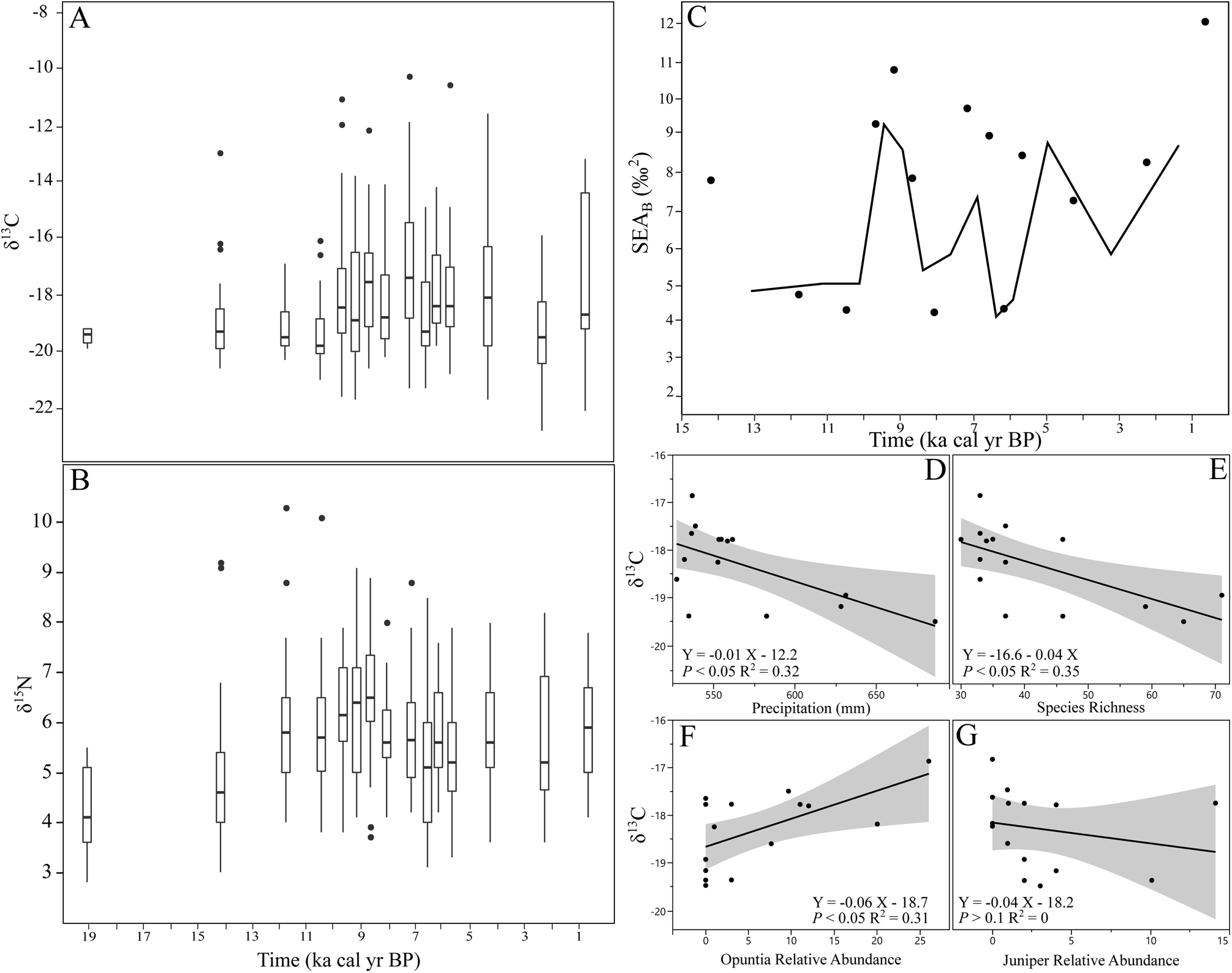
Figure 4. Temporal changes in Neotoma collagen isotopes. Boxplots give first and third quartiles, median, and 1.5 times the interquartile range (whiskers), with outliers (black circles) for (A) δ13C and (B) δ15N values. (C) Standard ellipse areas (SEAB in ‰2) and overlap of adjacent SEAB values (solid line) through time. Linear relationships between (D) mean annual precipitation, (E) local mammal species, relative pollen abundance of (F) Opuntia, and (G) Cupressaceae.
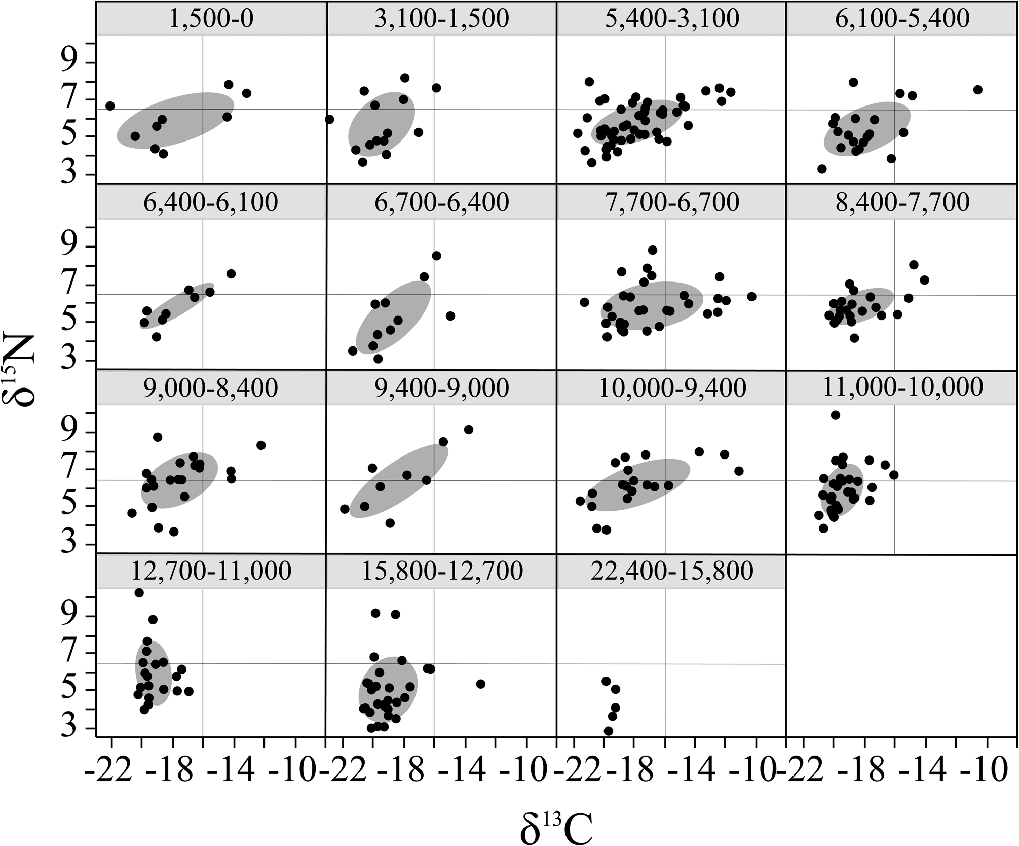
Figure 5. Temporal changes in the isotopic niche of Neotoma. Standard ellipse areas (SEAs) represent 50% coverage of population δ13C and δ15N values. Horizontal and vertical lines in each plot are included as a visual guide. SEA was not calculated for oldest time interval (22,400–15,800 cal yr BP) due to low sample size (N = 5).
δ13C values were significantly correlated with changes in vegetation. Neotoma consumed a higher proportion of C4/CAM plants, with increasing amounts of Opuntia (linear model F-statistic = 7.19, df = 1/13, p < 0.05, adjusted r2 = 0.31) and decreasing amounts of C3 grasses (linear model F-statistic = 9.95, df = 1/13, p < 0.01) on the landscape (Fig. 4F). We found no correlation between Neotoma isotope values and Cupressaceae pollen abundance (linear model F-statistic = 0.62, df = 1/13, p > 0.1; Fig. 4G).
DISCUSSION
Our results clearly show that Neotoma were sensitive to the climate and biodiversity changes of the terminal Pleistocene and early Holocene. As the glacial-era ice sheets retreated and climate warmed and dried, Neotoma became smaller (Fig. 3A) and incorporated a larger proportion of C4/CAM plants in their diet as these resources increased in availability on the landscape (Figs. 2D, 4F, 5). Decreased body size and greater mixed resource use also were associated with the loss and turnover in mammalian biodiversity (Supplementary Table S5; Figs. 3C, 4E). Whether these changes resulted from adaptation within a single species, as has been shown elsewhere (Brown and Lee, Reference Brown and Lee1969; Smith et al., Reference Smith, Betancourt and Brown1995, Reference Smith, Browning and Shepherd1998; Smith and Betancourt, Reference Smith and Betancourt1998, Reference Smith and Betancourt2003), or from the partial or full replacement of species within the genus is unclear, but overall we observed large shifts in the ecology of Neotoma as they responded to a combination of abiotic and biotic stressors.
Neotoma underwent significant decreases in body mass throughout the end of the Pleistocene and the Holocene (Fig. 3A). The decrease in the maximum body mass of Neotoma over time was predominantly associated with community composition becoming more similar to modern and decreasing regional precipitation (Fig. 3B, C; Supplementary Table S5). While greater precipitation was associated with large median and maximum body mass throughout most of the Hall's Cave record, increasing temperatures had a strong influence on decreasing maximum body mass during the time intervals prior to ca. 7000 cal yr BP, when individuals of the largest species (N. floridana) were likely most abundant. With the warming climate of the Holocene, thermal intolerance likely led to reduced body size in the largest individuals of Neotoma across time intervals, consistent with Bergmann's rule, as has been observed previously at other localities (Brown and Lee, Reference Brown and Lee1969; Smith et al., Reference Smith, Betancourt and Brown1995, Reference Smith, Browning and Shepherd1998; Smith and Betancourt, Reference Smith and Betancourt1998, Reference Smith and Betancourt2003). The influence of community turnover on both maximum and median body mass suggests that animals became smaller overall as the mammal community composition became more similar to modern (Supplementary Table S5). Decreased size may be advantageous for predator avoidance in small mammals (Stanley, Reference Stanley1973), or smaller size may have altered Neotoma's ability to compete for resources or habitat, given that larger size in modern Neotoma can act as a competitive advantage (Finley, Reference Finley1958; Cameron, Reference Cameron1971; Dial, Reference Dial1988). Smaller body mass in Neotoma may therefore have led to changes in biotic interactions, specifically intra- or interspecific resource competition, and contributed to observed shifts in diet.
The dietary (isotopic) niche of Neotoma also shifted across the past 22,000 years with changes in climate, biodiversity loss, and vegetation. The mean δ13C values of Neotoma across the entire temporal record at Hall's Cave were generally reflective of mixed use of C3 and C4/CAM resources ranging between -16.9 to -19.5‰ (SD: 0.3–3.1‰) (Table 1). The largest δ13C change occurs around the extinction event when Neotoma shift between consuming a greater proportion of C3 plants prior to the extinction to higher mixed C3-C4/CAM use during the Holocene (Table 1). Prior to 14,000 cal yr BP, the Edwards Plateau was covered in deciduous forest (Bryant and Holloway, Reference Bryant, Holloway, Bryant and Holloway1985), but a regional shift to warmer and drier conditions led to the expansion of grassland and oak savanna ecosystems by ca. 11,600 cal yr BP (Bryant and Holloway, Reference Bryant, Holloway, Bryant and Holloway1985). Over the Holocene, the Edwards Plateau became a more open savanna landscape and C4 vegetation continued to increase across Texas (Nordt et al., Reference Nordt, Boutton, Hallmark and Waters1994; Koch et al., Reference Koch, Diffenbaugh and Hoppe2004; Cotton et al., Reference Cotton, Cerling, Hoppe, Mosier and Still2016; Cordova and Johnson, Reference Cordova and Johnson2019). These changes occurred in concert with an increase in the isotopic niche (SEAB) of Neotoma beginning 10,000 years ago. Prior to this interval, C3 resources were ~55–60% of the diet of Neotoma, but use of C3 plants decreased slightly (to ~42–54%) for most of the Holocene, with the exception of 3100–1500 cal yr BP, when diet consisted of 59% C3 resources (Table 1). Following an increase in Opuntia abundance at ca. 9000 cal yr BP (Cordova and Johnson, Reference Cordova and Johnson2019; Fig. 2D), we find a parallel increase in the consumption of C4/CAM (58%) at 7700–6700 cal yr BP. A sudden decrease in SEAB between 6700–6400 cal yr BP (Fig. 4C; 5) coincides with the disappearance of Opuntia from the Hall's Cave fossil record (Fig 2D), and a shift away from a more mixed C3-C4/CAM diet to greater use of C3 resources (~54%, Table 1). As Opuntia reappears, the breadth of δ13C values of Neotoma increase as well (Figs. 2D, 4C, 5). These patterns suggest a strong influence of local vegetation composition and resource availability on the diet of Neotoma.
Temporal variation in Neotoma δ15N values (Figs. 4B, 5) potentially reflect changes in trophic level and/or baseline shifts in the nitrogen isotope composition of vegetation. Here, δ15N values of Neotoma collagen decreased over time and were positively correlated with higher δ13C values (Figs. 4B, 5). Tomé et al. (Reference Tomé, Elliott Smith, Lyons, Newsome and Smith2020a) found a similar pattern in the δ15N values for Sigmodon hispidus (hispid cotton rat) in the Hall's Cave record, an herbivorous rodent generally inhabiting grassland habitats (Cameron and Spencer, Reference Cameron and Spencer1981; Kincaid and Cameron, Reference Kincaid and Cameron1985; Randolph et al., Reference Randolph, Cameron and Wrazen1991; Toomey, Reference Toomey1993). Sigmodon δ15N values ranged between 5.5–7.4‰, and throughout the 14 time intervals that Sigmodon and Neotoma co-occur, their mean δ15N values were within 2‰ of each other and they had a similar degree of within-interval variance, suggesting they were likely feeding at similar trophic levels. Sigmodon was strongly influenced by shifts in community composition and resource availability such that the decrease in δ15N values in this omnivorous generalist corresponded with an increase in the proportion of insectivores on the landscape (Tomé et al., Reference Tomé, Elliott Smith, Lyons, Newsome and Smith2020a). Interestingly, a significant correlation between Neotoma δ15N and turnover (negative correlation) and similarity to modern (positive correlation) species composition in the community suggest that changes in resource use by Neotoma were linked to biotic interactions (i.e., competition). Omnivory in modern populations of Neotoma, however, is restricted to a very limited consumption of insects (Vorhies and Taylor, Reference Vorhies and Taylor1940; Rainey, Reference Rainey1956). The δ15N values of a consumer are typically enriched by ~3–5‰ compared to its diet (DeNiro and Epstein, Reference DeNiro and Epstein1981), and on the whole, the mean δ15N values of Neotoma varied by only 2.3‰ across all intervals, with the SD for any given time interval being below 2‰, suggesting the genus was unlikely to be switching between omnivorous and herbivorous diets. Comparison of Neotoma δ15N data with those of other obligate herbivores suggests that this degree of variation in δ15N is common in primary consumers. For example, bison δ15N values were 5.7–8.3‰ (±0.7–1.2‰) between ca. 6000–3100 cal yr BP and 5.7–6.2‰ (±0.5–0.9‰) between ca. 3100–500 cal yr BP across seven Texas cave sites (Lohse et al., Reference Lohse, Madsen, Culleton and Kennett2014), while Neotoma δ15N values were 5.4–5.8‰ (±1.1–1.3‰) between ca. 6100–3100 cal yr BP and 5.7–5.9‰ (±1.3–1.5‰) between ca. 3100–0 cal yr BP. Bison also show a positive correlation between δ13C and δ15N values and a significant decrease in δ15N values over the Holocene (Lohse et al., Reference Lohse, Madsen, Culleton and Kennett2014). The small range in Neotoma δ15N values and the correlation between increased C4 consumption and higher δ15N values in many time bins (Figs. 4B, 5) could therefore result from changing environmental conditions (DeNiro and Epstein, Reference DeNiro and Epstein1981; Amundson et al., Reference Amundson, Austin, Schuur, Yoo, Matzek, Kendall, Uebersax, Brenner and Baisden2003). In general, plant δ15N values increase with environmental aridity (Ambrose, Reference Ambrose1991; Austin and Vitousek, Reference Austin and Vitousek1998; Amundson et al., Reference Amundson, Austin, Schuur, Yoo, Matzek, Kendall, Uebersax, Brenner and Baisden2003). We found Neotoma δ15N values were positively correlated with increasing minimum temperature, suggesting plant δ15N increased as the environment warmed. However, we also found δ15N decreased with increasing maximum temperature, and we found no correlation between δ15N and precipitation (Supplementary Table S5), as may have been expected from modern patterns. Despite this, the lack of evidence for a trophic level shift and the similar patterns shown in herbivore nitrogen values from the region suggest changes in δ15N values of Neotoma at Hall's Cave were likely due to changes in the baseline nitrogen isotope composition of local vegetation.
Shifts in both body mass and diet of Neotoma also may be related to temporal changes in the species of Neotoma that were present at the site. Prior to the extinction event, the larger-bodied N. floridana was most likely the only species present, according to DNA work on fossils from the oldest strata (Seersholm et al., Reference Seersholm, Werndly, Grealy, Johnson, Keenan Early, Lundelius and Winsborough2020). From ca. 21,000–17,000 cal yr BP, the vegetation of the Edwards Plateau was deciduous forest, which is the preferred habitat for modern N. floridana (Rainey, Reference Rainey1956; Bryant and Holloway, Reference Bryant, Holloway, Bryant and Holloway1985). After 17,000 cal yr BP, the region shifted towards a more open grassland/savanna habitat (Bryant and Holloway, Reference Bryant, Holloway, Bryant and Holloway1985; Cordova and Johnson, Reference Cordova and Johnson2019), which is more characteristic of the habitat within the modern range of N. micropus and/or N. albigula (Finley, Reference Finley1958; Macêdo and Mares, Reference Macêdo and Mares1988; Braun and Mares, Reference Braun and Mares1989). Rapid decreases in precipitation and increasing temperature before ca. 9000 cal yr BP (Fig. 2A–C) were strongly correlated with decreases in maximum body mass (Supplementary Table S5) and may be a result of a lower abundance of N. floridana on the landscape. Increasing similarity of mammal species to modern community composition was also significantly and positively correlated to maximum body mass prior to ca. 7000 cal yr BP and to median body mass after ca. 9000–7000 cal yr BP, suggesting an important transition in the abundance and composition of Neotoma species present on the Edwards Plateau. Thus, colonization of the Edwards Plateau by smaller Neotoma species may have been facilitated by regional shifts in vegetation due to changing climate. The observed decrease in Neotoma body mass may be a consequence of an adaptation to increasing temperatures, but may also be related to the increased abundance of N. micropus and/or N. albigula in the Hall's Cave fossil record.
Changes in diet of Neotoma over time also may be related to differences in resource use among species in the genus. Today, both N. albigula and N. micropus consume high proportions of cacti (e.g., Opuntia; Finley, Reference Finley1958; Dial, Reference Dial1988; Macêdo and Mares, Reference Macêdo and Mares1988; Braun and Mares, Reference Braun and Mares1989). Drought-adapted CAM plants typically have δ13C values that are similar to C4 plants in arid land ecosystems; mean (±SE) δ13C values for Opuntia (prickly pear cacti) collected in Texas south of the Edwards Plateau were -15.6 ± 0.2‰ (Mooney et al., Reference Mooney, Troughton and Berry1974; Sutton et al., Reference Sutton, Ting and Troughton1976; Mooney et al., Reference Mooney, Bullock and Ehleringer1989; Boutton et al., Reference Boutton, Archer, Midwood, Zitzer and Bol1998). We found a significant and positive correlation between the increase in the amount of the Opuntia cactus in the region with (1) decreased precipitation (Fig. 2), and (2) higher Neotoma δ13C values (Fig. 4F). This shift in the δ13C values of Neotoma is indicative of greater use of C4/CAM resources. Additionally, regional vegetation shifts may have decreased the habitat and resources that N. floridana relies on for den building (e.g., fallen tree trunks and branches), and increased those (e.g., shrubs and cacti) used by N. micropus and/or N. albigula (Rainey, Reference Rainey1956; Finley, Reference Finley1958; Brown et al., Reference Brown, Lieberman and Dengler1972; Thies and Caire, Reference Thies and Caire1990). Reduced availability of appropriate building materials for den construction can lead to declines in modern Neotoma populations, generally related to reduced thermal and predator protection (Raun, Reference Raun1966; Brown, Reference Brown1968; Brown et al., Reference Brown, Lieberman and Dengler1972; Smith, Reference Smith1995b; Ford et al., Reference Ford, Castleberry, Mengak, Rodrigue, Feller and Russell2006). We also found that while the presence of cacti was significantly correlated with shifts in Neotoma diet, juniper (Cupressaceae) abundance was not. Of these three species, N. albigula makes the most use of juniper, which can represent as much as 35% of the diet in some populations (Finley, Reference Finley1958). The lack of correlation with changes in juniper and diet (Fig. 4G) may suggest that N. albigula was present in lower abundance than N. micropus in the Hall's Cave record after ca. 6700 cal yr BP, potentially because the larger-bodied N. micropus outcompeted smaller-bodied species for space and resources (Finley, Reference Finley1958; Cameron, Reference Cameron1971; Dial Reference Dial1988). We also found no overall correlation between body size and diet (Supplementary Table S6), despite shifts towards smaller size and higher C4/CAM consumption over time. It is possible that variation in resource use within one or more species of Neotoma is partially responsible for change in δ13C values, as shown by small-mammal studies that reported wide resource use even in what are considered to be dietary specialists (Terry et al., Reference Terry, Guerre and Taylor2017, Terry, Reference Terry2018). However, if N. micropus abundances were higher than those N. albigula, the larger overlap in mass with co-occurring N. floridana may mask changes at the species level versus wider resource use at the genus level.
Overall, Neotoma responses suggest a strong abiotic influence from climate at the terminal Pleistocene, and likely changes in relative abundance from N. floridana to N. micropus and/or N. albigula in the Holocene associated with changing local resource availability. Climatic fluctuations and ecosystem disruption due to the megafauna extinction event may both have played roles in vegetation shifts (Owen-Smith, Reference Owen-Smith1992), which led to a change in relative abundances of Neotoma species as habitat and resources became more suitable to the two arid-adapted species. Differences in how Neotoma responded to community and climatic changes across the Hall's Cave record suggest that the strength of abiotic and biotic effects on a species can vary over time. Characterization of a genus’ or species’ niche(s) through time can therefore provide insight into the regional vegetational and community shifts produced as a consequence of large-scale abiotic and biotic changes, which can inform how modern communities may respond to modern anthropogenic climate change and biodiversity loss.
Supplementary Material
The supplementary material for this article can be found at https://doi.org/10.1017/qua.2021.29.
Acknowledgments
We thank the staff at the Texas Memorial Museum for access to their fabulous collections and their expertise and help; we are particularly grateful to Drs. Chris Sagebiel and Ernie Lundelius for their willingness to assist us with locating references, specimens, and information about the sites. We also thank Dr. Thomas W. Stafford Jr. at Stafford Research for his input, enthusiasm, and work with the Hall's Cave fossil record; this project would not have been possible without his assistance. The Museum of Southwestern Biology and the Senior Collection Manager of Mammals, Dr. Jon Dunnum, provided access to the modern collections at UNM. We would also like to thank Dr. Rickard Toomey for his foundational excavations and work at Hall's Cave, which made our project possible, and the owners of the private ranch on which Hall's Cave is located for having graciously allowed generations of paleontologists to work at this very important late Quaternary fossil site. Finally, thanks to the many members of the Smith lab at UNM, especially Jonathan Keller, who assisted with revisions of the age model.
Financial Support
Funding for this project was provided by NSF-DEB 1555525 and 1744223 (FA Smith, PI; SD Newsome, SK Lyons co-PIs).
Data Availability
Data are available from the Dryad Digital Repository: Tomé, Catalina P.; Lyons, S. Kathleen; Newsome, Seth D.; Smith, Felisa A. (2021), Data from: The sensitivity of Neotoma to climate change and biodiversity loss over the late Quaternary, Dryad, Dataset, https://doi.org/105061/dryad.4j0zpc8b3.


