


1. Introduction
Nonlinear water waves in intricate domains is a theme of great physical interest. In this topic, nonlinear wave problems generally occur when the bathymetry is variable. The solitary wave is a reference nonlinear wave in these studies. There is a great deal of literature, and we point out a few works: Mei & Hancock (Reference Mei and Hancock2003), Nachbin (Reference Nachbin2003), Muñoz & Nachbin (Reference Muñoz and Nachbin2005), Garnier et al. (Reference Garnier, Muñoz and Nachbin2007) and Grimshaw & Annenkov (Reference Grimshaw and Annenkov2007), all related to waves in the presence of a variable topography. Many other relevant articles can be found, for example, in the references of the above publications. Surprisingly, another topic in this class of problems does not feature much in the literature, regarding either its physical or mathematical aspects: solitary waves propagating in intricate channel networks (Harbitz Reference Harbitz1992; Shi, Teng & Wu Reference Shi, Teng and Wu1998; Shi, Teng & Sou Reference Shi, Teng and Sou2005; Harbitz et al. Reference Harbitz, Glimsdal, Løvhot, Kveldsvik, Pedersen and Jensen2014). A problem that is addressed here for the first time concerns the reduction of a two-dimensional (2D) nonlinear dispersive wave model into an effective one-dimensional (1D) system, defined on a network. Tsunami propagation on a channel network has not seen much theoretical investigation. One relevant application is to tsunamis in fjords, as observed in Norway. Information on this is provided by the Norwegian Geotechnical Institute (NGI) at their website under Monitoring and modelling of the Åknes. The fjords have sharp turns and branch out into a complicated domain where large waves can propagate for long distances (Nachbin & Simões Reference Nachbin and Simões2012; Harbitz et al. Reference Harbitz, Glimsdal, Løvhot, Kveldsvik, Pedersen and Jensen2014). In 1934 more than 40 people were killed when a tsunami destroyed the Tafjord village. This village was tens of kilometres away from a landslide, which created a tsunami arriving at Tafjord with a height of 16 m. These large waves will eventually break, the dynamics is highly non-trivial, and we begin our study of large and localized disturbances with solitary waves.
The case of open channels with sharp turns was studied by Harbitz (Reference Harbitz1992) and Shi et al. (Reference Shi, Teng and Wu1998), who identified the different reflection characteristics for solitary waves. A channel was considered to be narrow when
 $L/{\it\lambda}_{e}$
is small, where
$L/{\it\lambda}_{e}$
is small, where
 $L$
is the channel width and
$L$
is the channel width and
 ${\it\lambda}_{e}$
the solitary wave’s effective width. Shi et al. (Reference Shi, Teng and Wu1998) showed that when the channel is narrow no reflection is produced at a sharp turn, in contrast to moderate and wide channels where a non-trivial reflected wave is observed. The absence of reflection for narrow channels was rationalized in a recent article by the present authors (Nachbin & Simões Reference Nachbin and Simões2012). As will be shown in the present work, narrow branching channels generally produce a reflected wave.
${\it\lambda}_{e}$
the solitary wave’s effective width. Shi et al. (Reference Shi, Teng and Wu1998) showed that when the channel is narrow no reflection is produced at a sharp turn, in contrast to moderate and wide channels where a non-trivial reflected wave is observed. The absence of reflection for narrow channels was rationalized in a recent article by the present authors (Nachbin & Simões Reference Nachbin and Simões2012). As will be shown in the present work, narrow branching channels generally produce a reflected wave.
The study presented in Nachbin & Simões (Reference Nachbin and Simões2012) allowed the authors to consider the more challenging case of solitary waves propagating through a forked region of a channel network. Many applications can be considered, ranging from the more obvious case of waves in man-made channel networks to tsunamis in fjords, as mentioned above. Having an efficient model, through which one can assess both the physical and mathematical properties of this complicated dynamics, is of great interest and largely unexplored. A wave model on a 1D network reduces the geometrical complexity of the problem. To the best of our knowledge there are very few references on water waves in networks (Jacovkis Reference Jacovkis1991; Bona & Cascaval Reference Bona and Cascaval2008). The former reference considers linear (hyperbolic) waves while the latter considers solitary waves but with no reflection mechanism. Moreover, there is no mathematical model available which incorporates the effect of angles at the branching point as well as asymmetric branching configurations as described below. We present the first model, which has this information built into the system of differential equations, in a natural and systematic fashion, through an appropriate choice of coordinate system and its corresponding Jacobian.
With this in mind, we start with a 2D Boussinesq-type model (Wu Reference Wu1981) and formulate a reduced 1D model that captures the main features of this non-trivial dynamics. Moreover, our reduced 1D model captures the influence of different branching angles, in both a symmetric (Y-like) and an asymmetric configuration, where there is a main reach and a new reach emerges from it, as in figure 1. Our results concern a nonlinear water wave model for the reflection and transmission of solitary waves on a graph, which hopefully will stimulate further research. In particular, a compatibility condition is needed at the nodes of the graph. We point out that the present model allows reaches of three different widths. Here, for simplicity with regard to mathematical theory, we take the three reaches at a branching point to have the same width
 $L$
.
$L$
.

Figure 1. A solitary wave enters the domain from the right, propagating to the left, and crosses the forked region of a 2D channel. Two transmitted pulses are seen: one through the main reach and the other through a reach at 60°. A reflected depression wave is observed propagating back to the right.
The results of this paper are summarized as follows.
-
(i) Through a conformal mapping, 2D forked regions are considered at any branching angle
 ${\it\alpha}$
. Previous studies in Cartesian coordinates were restricted (for meshing reasons) to angles that were multiples of
${\rm\pi}/4$
(Shi et al.
Reference Shi, Teng and Sou2005).
${\it\alpha}$
. Previous studies in Cartesian coordinates were restricted (for meshing reasons) to angles that were multiples of
${\rm\pi}/4$
(Shi et al.
Reference Shi, Teng and Sou2005). -
(ii) On a graph/network-like domain, a new 1D Boussinesq model is deduced, which includes angle information from the forked region. No previous 1D model has this information built into the equations (Jacovkis Reference Jacovkis1991; Bona & Cascaval Reference Bona and Cascaval2008).
-
(iii) A new three-point nonlinear compatibility condition is presented. It proves to be more general and more accurate than the existing/standard one-point linear compatibility condition (Stoker Reference Stoker1957; Jacovkis Reference Jacovkis1991; Bona & Cascaval Reference Bona and Cascaval2008).
-
(iv) No previous study has compared the 2D and 1D solutions.


This paper is organized as follows. In § 2 the 2D Boussinesq (long-wave) system deduced by Wu (Reference Wu1981) is introduced, as well as our conformal mapping. With the conformal mapping we generalize this wave model to better accommodate channels with a larger range of branching angles as well as to further simplify it to a 1D wave model on a graph. In § 3 the 2D Boussinesq system is reduced to a 1D wave system through transversal averaging. Most importantly, a compatibility condition is needed at the node of the underlying graph-like 1D domain. A well-known compatibility condition is revisited and compared with our new compatibility conditions. Numerical simulations illustrate the improved accuracy of the new compatibility conditions. We identify the regime where asymmetry manifests itself in the reflection–transmission dynamics.
2. The 2D Boussinesq model
Consider an open channel of constant rectangular cross-section, of width
 $L$
and undisturbed depth
$L$
and undisturbed depth
 $h_{0}$
. Starting from the three-dimensional formulation of nonlinear potential theory (Mei, Stiassnie & Yue Reference Mei, Stiassnie and Yue2005), Wu (Reference Wu1981) obtained the generalized Boussinesq system
$h_{0}$
. Starting from the three-dimensional formulation of nonlinear potential theory (Mei, Stiassnie & Yue Reference Mei, Stiassnie and Yue2005), Wu (Reference Wu1981) obtained the generalized Boussinesq system
 $$\begin{eqnarray}\displaystyle & {\it\eta}_{t}+(1+{\it\eta})({\it\phi}_{xx}+{\it\phi}_{yy})+{\it\eta}_{x}{\it\phi}_{x}+{\it\eta}_{y}{\it\phi}_{y}=0, & \displaystyle\end{eqnarray}$$
 $$\begin{eqnarray}\displaystyle & \displaystyle {\it\phi}_{t}+{\it\eta}+\frac{{\it\phi}_{x}^{2}+{\it\phi}_{y}^{2}}{2}-\frac{{\it\phi}_{xxt}+{\it\phi}_{yyt}}{3}=0. & \displaystyle\end{eqnarray}$$
 ${\it\eta}(x,y,t)$
. The horizontal velocity field is obtained from the vertically averaged potential,
${\it\eta}(x,y,t)$
. The horizontal velocity field is obtained from the vertically averaged potential,
 $(u,v)=\boldsymbol{{\rm\nabla}}{\it\phi}$
. In other words the reduced potential
$(u,v)=\boldsymbol{{\rm\nabla}}{\it\phi}$
. In other words the reduced potential
 ${\it\phi}(x,y,t)$
is obtained from the velocity potential
${\it\phi}(x,y,t)$
is obtained from the velocity potential
 ${\it\Phi}(x,y,z,t)$
, once it has been vertically averaged over the fluid body. For the reduced potential
${\it\Phi}(x,y,z,t)$
, once it has been vertically averaged over the fluid body. For the reduced potential
 ${\it\phi}$
a Neumann condition is imposed along the side walls of the channel, which are impermeable and very high; the model does not account for spilling out of the bed. We have normalized the reference shallow water speed to be
${\it\phi}$
a Neumann condition is imposed along the side walls of the channel, which are impermeable and very high; the model does not account for spilling out of the bed. We have normalized the reference shallow water speed to be
 $c_{o}=\sqrt{gh_{0}}=1$
. An approximate solitary wave solution is available for this model (Shi et al.
Reference Shi, Teng and Sou2005):
$c_{o}=\sqrt{gh_{0}}=1$
. An approximate solitary wave solution is available for this model (Shi et al.
Reference Shi, Teng and Sou2005):  $$\begin{eqnarray}\displaystyle & \displaystyle {\it\eta}(x,t)=\frac{a\text{ sech}^{2}b(x-x_{0}-ct)}{1+a\text{ tanh}^{2}b(x-x_{0}-ct)}, & \displaystyle\end{eqnarray}$$
 $$\begin{eqnarray}\displaystyle & \displaystyle {\it\phi}(x,t)=\frac{ca}{b(1+a)}\text{tanh}\;b(x-x_{0}-ct), & \displaystyle\end{eqnarray}$$
 $b(a)=\sqrt{3a/4(1+0.68a)}$
and
$b(a)=\sqrt{3a/4(1+0.68a)}$
and
 $x_{0}$
is the solitary wave’s initial position. The amplitude-dependent wave speed is
$x_{0}$
is the solitary wave’s initial position. The amplitude-dependent wave speed is  $$\begin{eqnarray}c(a)=\sqrt{[(1+a)\ln (1+a)-a]6(1+a)^{2}/[a^{2}(3+2a)]}.\end{eqnarray}$$
This is an exact travelling wave for an underlying second-order differential equation. In Shi et al. (Reference Shi, Teng and Sou2005) the effective wavelength
 ${\it\lambda}_{e}$
of the solitary wave is defined as being the length within which the solitary wave elevation is larger than 1 % of its amplitude
${\it\lambda}_{e}$
of the solitary wave is defined as being the length within which the solitary wave elevation is larger than 1 % of its amplitude
 $a$
. Based on our previous numerical experience (Nachbin & Simões Reference Nachbin and Simões2012) we take the amplitude to be
$a$
. Based on our previous numerical experience (Nachbin & Simões Reference Nachbin and Simões2012) we take the amplitude to be
 $a=0.3$
, while the wavelength is respectively
$a=0.3$
, while the wavelength is respectively
 ${\it\lambda}_{e}\approx 13$
.
${\it\lambda}_{e}\approx 13$
.
We have checked that along a 2D uniform channel this profile is a very good approximation of a solitary travelling wave. Therefore it is used in our numerical experiments with solitary waves in branching channels. A snapshot of such an experiment is shown in figure 1, where the solitary wave gives rise to two transmitted pulses, one along the main reach and a slightly smaller pulse along the branching reach at 60°.
2.1. A convenient change of coordinate system
We now change coordinate systems. Recall the typical notation for a conformal map
 $z=F(w)$
, where
$z=F(w)$
, where
 $w={\it\xi}+\text{i}{\it\zeta}$
and
$w={\it\xi}+\text{i}{\it\zeta}$
and
 $z=x+\text{i}y$
. The mapping is taken from a uniform (canonical) strip in the complex
$z=x+\text{i}y$
. The mapping is taken from a uniform (canonical) strip in the complex
 $w$
-plane onto a Y-shaped ‘strip’ in the complex
$w$
-plane onto a Y-shaped ‘strip’ in the complex
 $z$
-plane. These are depicted in figure 2. By using the conformal mapping’s coordinate system we allow for a better understanding of the reflection and transmission problem, as well as its reduction to a simpler 1D, graph-like model. As will be reported in this paper, the Schwarz–Christoffel transformation (Driscoll & Trefethen Reference Driscoll and Trefethen2002) is specially tailored for polygonal-shaped regions such as near the forked region. The following expressions are useful (Nachbin Reference Nachbin2003):
$z$
-plane. These are depicted in figure 2. By using the conformal mapping’s coordinate system we allow for a better understanding of the reflection and transmission problem, as well as its reduction to a simpler 1D, graph-like model. As will be reported in this paper, the Schwarz–Christoffel transformation (Driscoll & Trefethen Reference Driscoll and Trefethen2002) is specially tailored for polygonal-shaped regions such as near the forked region. The following expressions are useful (Nachbin Reference Nachbin2003):
 ${\it\phi}_{x}^{}=[x_{{\it\xi}}{\it\phi}_{{\it\xi}}^{}+x_{{\it\zeta}}{\it\phi}_{{\it\zeta}}^{}]/|J|$
,
${\it\phi}_{x}^{}=[x_{{\it\xi}}{\it\phi}_{{\it\xi}}^{}+x_{{\it\zeta}}{\it\phi}_{{\it\zeta}}^{}]/|J|$
,
 ${\it\phi}_{y}^{}=[y_{{\it\xi}}{\it\phi}_{{\it\xi}}^{}+y_{{\it\zeta}}{\it\phi}_{{\it\zeta}}^{}]/|J|,$
and
${\it\phi}_{y}^{}=[y_{{\it\xi}}{\it\phi}_{{\it\xi}}^{}+y_{{\it\zeta}}{\it\phi}_{{\it\zeta}}^{}]/|J|,$
and
 $|J|=y_{{\it\xi}}^{2}+y_{{\it\zeta}}^{2}$
, together with the Cauchy–Riemann equations. In the orthogonal curvilinear coordinate system
$|J|=y_{{\it\xi}}^{2}+y_{{\it\zeta}}^{2}$
, together with the Cauchy–Riemann equations. In the orthogonal curvilinear coordinate system
 $({\it\xi},{\it\zeta})$
, the generalized Boussinesq system becomes
$({\it\xi},{\it\zeta})$
, the generalized Boussinesq system becomes
 $$\begin{eqnarray}\displaystyle & |J|{\it\eta}_{t}+(1+{\it\eta})({\it\phi}_{{\it\xi}{\it\xi}}+{\it\phi}_{{\it\zeta}{\it\zeta}})+{\it\eta}_{{\it\xi}}{\it\phi}_{{\it\xi}}+{\it\eta}_{{\it\zeta}}{\it\phi}_{{\it\zeta}}=0, & \displaystyle\end{eqnarray}$$
 $$\begin{eqnarray}\displaystyle & \displaystyle {\it\phi}_{t}+{\it\eta}+\frac{{\it\phi}_{{\it\xi}}^{2}+{\it\phi}_{{\it\zeta}}^{2}}{2|J|}-\frac{{\it\phi}_{{\it\xi}{\it\xi}t}+{\it\phi}_{{\it\zeta}{\it\zeta}t}}{3|J|}=0. & \displaystyle\end{eqnarray}$$

Figure 2. From top to bottom we have three non-trivial channel configurations: an abrupt turn at 90°, a symmetric branching channel with angles
 $\pm {\it\alpha}$
, and an asymmetric branching channel of angle
$\pm {\it\alpha}$
, and an asymmetric branching channel of angle
 ${\it\alpha}$
. (a) The physical channels; (b) the canonical channels (in the
${\it\alpha}$
. (a) The physical channels; (b) the canonical channels (in the
 $w$
-plane). The slits in the canonical channels indicate the segment where the two reaches meet, after the branches have been ‘closed’ by the inverse mapping.
$w$
-plane). The slits in the canonical channels indicate the segment where the two reaches meet, after the branches have been ‘closed’ by the inverse mapping.
Conserved quantities such as the excess mass, due to the wave elevation, and the total energy are expressed as
 $M(t)=\!\int \!\!\int _{\!{\it\Omega}}\!{\it\eta}|J|\,\text{d}{\it\xi}\,\text{d}{\it\zeta}$
,
$M(t)=\!\int \!\!\int _{\!{\it\Omega}}\!{\it\eta}|J|\,\text{d}{\it\xi}\,\text{d}{\it\zeta}$
,
 $E(t)=\!\int \!\!\int _{\!{\it\Omega}}({\it\eta}^{2}|J|+{\it\phi}_{{\it\xi}}^{2}\!+{\it\phi}_{{\it\zeta}}^{2})/2\,\text{d}{\it\xi}\,\text{d}{\it\zeta}$
, where
$E(t)=\!\int \!\!\int _{\!{\it\Omega}}({\it\eta}^{2}|J|+{\it\phi}_{{\it\xi}}^{2}\!+{\it\phi}_{{\it\zeta}}^{2})/2\,\text{d}{\it\xi}\,\text{d}{\it\zeta}$
, where
 ${\it\Omega}$
is the entire forked region considered. This variable coefficient Boussinesq system has already been studied for channels with abrupt turns by Nachbin & Simões (Reference Nachbin and Simões2012), who verified the numerical method’s energy-preserving properties in the presence of a non-trivial
${\it\Omega}$
is the entire forked region considered. This variable coefficient Boussinesq system has already been studied for channels with abrupt turns by Nachbin & Simões (Reference Nachbin and Simões2012), who verified the numerical method’s energy-preserving properties in the presence of a non-trivial
 $|J|$
. It was pointed out that in the new coordinate system the reciprocal of the Jacobian
$|J|$
. It was pointed out that in the new coordinate system the reciprocal of the Jacobian
 $|J|$
plays a role similar to a topography, as studied earlier by one of the authors (Nachbin Reference Nachbin2003; Garnier et al.
Reference Garnier, Muñoz and Nachbin2007). This useful interpretation can again be applied in the present case of branching channels, as depicted in figure 3. The Jacobian viewed in this figure can be associated with a step-like topography. One way to get a feel for how the heterogeneous medium’s variation affects propagation is to observe the presence of a variable propagation speed in connection with the wave equation:
$|J|$
plays a role similar to a topography, as studied earlier by one of the authors (Nachbin Reference Nachbin2003; Garnier et al.
Reference Garnier, Muñoz and Nachbin2007). This useful interpretation can again be applied in the present case of branching channels, as depicted in figure 3. The Jacobian viewed in this figure can be associated with a step-like topography. One way to get a feel for how the heterogeneous medium’s variation affects propagation is to observe the presence of a variable propagation speed in connection with the wave equation:
 $$\begin{eqnarray}{\it\eta}_{tt}-\left(\frac{1}{|J|({\it\xi},{\it\zeta})}\right){\rm\Delta}{\it\eta}=0.\end{eqnarray}$$
This wave equation is easily obtained by eliminating
 ${\it\phi}$
from the linear, non-dispersive version of (2.6)–(2.7). This variable-coefficient wave equation clearly indicates how system (2.6)–(2.7) has built into its coefficients reflection–transmission mechanisms at the branching region. Use of these boundary-fitted coordinates moved geometrical features along the boundary to algebraic (coefficient-based) data and allowed for new results with the underlying 1D forked graph, as will be described. In particular, it allowed for a systematic inclusion of angle and asymmetry information, which is not available in previous models of this kind.
${\it\phi}$
from the linear, non-dispersive version of (2.6)–(2.7). This variable-coefficient wave equation clearly indicates how system (2.6)–(2.7) has built into its coefficients reflection–transmission mechanisms at the branching region. Use of these boundary-fitted coordinates moved geometrical features along the boundary to algebraic (coefficient-based) data and allowed for new results with the underlying 1D forked graph, as will be described. In particular, it allowed for a systematic inclusion of angle and asymmetry information, which is not available in previous models of this kind.

Figure 3. The Jacobian
 $|J|=|J|({\it\xi},{\it\zeta})$
for an asymmetric branching channel of width
$|J|=|J|({\it\xi},{\it\zeta})$
for an asymmetric branching channel of width
 $L=1$
, having the secondary reach at an angle of
$L=1$
, having the secondary reach at an angle of
 ${\it\alpha}={\rm\pi}/2$
. The main reach is against the back wall of the figure in a configuration similar to figure 1. The Jacobian very quickly adjusts to a constant value along each reach.
${\it\alpha}={\rm\pi}/2$
. The main reach is against the back wall of the figure in a configuration similar to figure 1. The Jacobian very quickly adjusts to a constant value along each reach.
Before presenting the reduced 1D model on a graph we should mention that we carefully compared simulations performed with both system (2.1)–(2.2) and system (2.6)–(2.7) having exactly the same data. These were done for angles
 ${\it\alpha}={\rm\pi}/4$
and
${\it\alpha}={\rm\pi}/4$
and
 ${\it\alpha}={\rm\pi}/2$
where the Cartesian coordinate model will perform more easily, due to the positioning of numerical nodes along the side walls of the branching reach. Energy conservation was verified in both configurations and the solutions were basically the same. We also tested many different angle values as well as the conformal-mapping-based smoothing of corners, as reported in Nachbin & Simões (Reference Nachbin and Simões2012). This is achieved by having a slightly wider branching region mapped, followed by choosing the nearest
${\it\alpha}={\rm\pi}/2$
where the Cartesian coordinate model will perform more easily, due to the positioning of numerical nodes along the side walls of the branching reach. Energy conservation was verified in both configurations and the solutions were basically the same. We also tested many different angle values as well as the conformal-mapping-based smoothing of corners, as reported in Nachbin & Simões (Reference Nachbin and Simões2012). This is achieved by having a slightly wider branching region mapped, followed by choosing the nearest
 ${\it\zeta}$
-level curve as the channel’s boundary. In the Cartesian configuration, Shi et al. (Reference Shi, Teng and Sou2005) report having to perform an ad hoc averaging near the inner branching corner to avoid spurious oscillations. We observed and removed these oscillations with a very mild smoothing of the corner through the mapping of a slightly wider region. Hence the singularity of the mapping is very near to but outside the flow domain.
${\it\zeta}$
-level curve as the channel’s boundary. In the Cartesian configuration, Shi et al. (Reference Shi, Teng and Sou2005) report having to perform an ad hoc averaging near the inner branching corner to avoid spurious oscillations. We observed and removed these oscillations with a very mild smoothing of the corner through the mapping of a slightly wider region. Hence the singularity of the mapping is very near to but outside the flow domain.
Moreover, as already observed in Nachbin & Simões (Reference Nachbin and Simões2012), the wave dynamics just a short distance away from the forked region is basically 1D, quickly adjusting to the waveguide. This feature, further discussed via figure 4, called for a transversal averaging of the present model, which is very easily done in the mapped configuration since it amounts to averaging over
 ${\it\zeta}$
. The next section is on this reduction to a 1D model.
${\it\zeta}$
. The next section is on this reduction to a 1D model.

Figure 4. Asymmetric 2D forked channel of width
 $L=3$
and angle
$L=3$
and angle
 ${\it\alpha}={\rm\pi}/6$
. The 2D solitary wave is displayed at three different moments (
${\it\alpha}={\rm\pi}/6$
. The 2D solitary wave is displayed at three different moments (
 $t=28$
, 42, 46) and different plotting perspectives for better visualization. (a–c) Approaching the forked region from the right (a), at the forked region (b), and just after it has branched into two transmitted waves (c). A darker centre line highlights certain features discussed.
$t=28$
, 42, 46) and different plotting perspectives for better visualization. (a–c) Approaching the forked region from the right (a), at the forked region (b), and just after it has branched into two transmitted waves (c). A darker centre line highlights certain features discussed.
3. A reduced Boussinesq system on a branching graph
In our 2D simulations it has been observed that the wave dynamics is effectively 1D away from both an abrupt turning region (Nachbin & Simões Reference Nachbin and Simões2012) and a branching region. In figure 4, note the 2D solitary wave at three different moments: approaching the forked region from the right (figure 4
a), at the forked region (figure 4
b), and just after it has branched into two transmitted waves (figure 4
c). Different plotting perspectives were used, for better visualization of the comments to follow. The incoming wave is obviously a plane wave, well described by a 1D wave. As it goes through the forked region, the transmitted profile is primarily 1D. Surprisingly the transmitted pulse, arising from a solitary wave, quickly adjusts to the waveguide. The thicker lines highlight this observation. In figure 4(c) the development of the reflected wave clearly has more 2D components. Note that the channel width is not so small, being taken as
 $L=3$
in this example. We will show that transversal averaging of the 2D model, with an appropriate (new) nonlinear compatibility condition, captures very well the effective features of this problem, even when
$L=3$
in this example. We will show that transversal averaging of the 2D model, with an appropriate (new) nonlinear compatibility condition, captures very well the effective features of this problem, even when
 $L=5$
. Our main interest is focused on the transmitted pulse-shaped waves, namely the higher-amplitude components of the wavefield. A 1D reduction of model (2.6)–(2.7) follows, noting that we accept giving up non-dominant 2D features of the flow, which take place mostly in the grey area depicted in figure 6(c) and affect predominantly the small reflected wave. With regard to applications, it is of interest to have a good approximate value for the dominant wave, namely regarding the amplitude of the transmitted pulse along each reach. This is valuable information in a hazardous situation.
$L=5$
. Our main interest is focused on the transmitted pulse-shaped waves, namely the higher-amplitude components of the wavefield. A 1D reduction of model (2.6)–(2.7) follows, noting that we accept giving up non-dominant 2D features of the flow, which take place mostly in the grey area depicted in figure 6(c) and affect predominantly the small reflected wave. With regard to applications, it is of interest to have a good approximate value for the dominant wave, namely regarding the amplitude of the transmitted pulse along each reach. This is valuable information in a hazardous situation.
In the curvilinear coordinate system (or equivalently in the canonical domain) the lateral averaging is much simpler than with Cartesian coordinates, since it is performed only in the
 ${\it\zeta}$
-direction. Define this average by
${\it\zeta}$
-direction. Define this average by
 $\bar{f}({\it\xi})=(1/{\it\chi}_{j})\int _{[I]_{j}}f({\it\xi},{\it\zeta})\,\text{d}{\it\zeta}$
, where
$\bar{f}({\it\xi})=(1/{\it\chi}_{j})\int _{[I]_{j}}f({\it\xi},{\it\zeta})\,\text{d}{\it\zeta}$
, where
 $[I]_{j}$
denotes the transverse interval (in terms of
$[I]_{j}$
denotes the transverse interval (in terms of
 ${\it\zeta}$
) along the respective reach
${\it\zeta}$
) along the respective reach
 $j$
of canonical width
$j$
of canonical width
 ${\it\chi}_{j}<1$
. The canonical strip is normalized to be always of unit width. In the canonical
${\it\chi}_{j}<1$
. The canonical strip is normalized to be always of unit width. In the canonical
 $w$
-plane the normalized strip has
$w$
-plane the normalized strip has
 ${\it\chi}_{j}\neq L_{j}$
, where in the present study we chose
${\it\chi}_{j}\neq L_{j}$
, where in the present study we chose
 $L_{j}\equiv L$
. The numbering of each reach
$L_{j}\equiv L$
. The numbering of each reach
 $j$
is according to figure 6. As depicted in the upper part of figure 5, the canonical width of reach 2 is
$j$
is according to figure 6. As depicted in the upper part of figure 5, the canonical width of reach 2 is
 ${\it\chi}_{2}={\it\chi}$
. Clearly
${\it\chi}_{2}={\it\chi}$
. Clearly
 ${\it\chi}_{3}=1-{\it\chi}$
, recalling that the numerical Schwarz–Christoffel mapping normalizes the canonical strip to have unit width. An expression for these values will be presented later in this paper. In the long-wave/narrow-channel regime (where
${\it\chi}_{3}=1-{\it\chi}$
, recalling that the numerical Schwarz–Christoffel mapping normalizes the canonical strip to have unit width. An expression for these values will be presented later in this paper. In the long-wave/narrow-channel regime (where
 $L/{\it\lambda}_{e}={\it\varepsilon}$
, small) we observed that away from a neighbourhood around the branching region the transversal velocity
$L/{\it\lambda}_{e}={\it\varepsilon}$
, small) we observed that away from a neighbourhood around the branching region the transversal velocity
 $v={\it\phi}_{{\it\zeta}}$
is small and varies by a small amount in
$v={\it\phi}_{{\it\zeta}}$
is small and varies by a small amount in
 ${\it\zeta}$
. The flow field, generated by the presence of the wave in the forked region, is depicted in figure 5(b). The velocity field is mostly aligned with the level curves of constant
${\it\zeta}$
. The flow field, generated by the presence of the wave in the forked region, is depicted in figure 5(b). The velocity field is mostly aligned with the level curves of constant
 ${\it\zeta}$
-values and nearly constant along each transverse direction (i.e.
${\it\zeta}$
-values and nearly constant along each transverse direction (i.e.
 ${\it\xi}=\text{const.}$
). This is observed along (transversal) arch-like patterns having similar-sized velocity vectors.
${\it\xi}=\text{const.}$
). This is observed along (transversal) arch-like patterns having similar-sized velocity vectors.

Figure 5. (a) Branching region mapped to the canonical domain of unit width. The lower part of the channel, below the dashed line (i.e. the pre-image of the ‘separatrix’), has width
 ${\it\chi}$
. The three arrows indicate schematically the flux across the ‘separatrix’ as highlighted by the circle in (b). (b) Forked region with
${\it\chi}$
. The three arrows indicate schematically the flux across the ‘separatrix’ as highlighted by the circle in (b). (b) Forked region with
 ${\it\alpha}={\rm\pi}/2$
: velocity field due to the presence of the solitary wave at the branching region. Note the flux across the ‘separatrix’ (dashed line, defined as the
${\it\alpha}={\rm\pi}/2$
: velocity field due to the presence of the solitary wave at the branching region. Note the flux across the ‘separatrix’ (dashed line, defined as the
 ${\it\zeta}\equiv {\it\chi}$
level curve which connects to the inner corner).
${\it\zeta}\equiv {\it\chi}$
level curve which connects to the inner corner).

Figure 6. (a) Reaches in the canonical 2D domain; the dots indicate the points
 $p_{1}$
,
$p_{1}$
,
 $p_{2}$
and
$p_{2}$
and
 $p_{3}$
in the nonlinear compatibility conditions (3.6)–(3.8). (b) Configuration for the linear compatibility conditions (3.3)–(3.4). (c) Configuration for the nonlinear compatibility conditions (3.6)–(3.8).
$p_{3}$
in the nonlinear compatibility conditions (3.6)–(3.8). (b) Configuration for the linear compatibility conditions (3.3)–(3.4). (c) Configuration for the nonlinear compatibility conditions (3.6)–(3.8).
Based on the observations above it is natural to write
 ${\it\phi}_{{\it\zeta}}\approx {\it\varepsilon}v({\it\xi},{\it\varepsilon}{\it\zeta},t)$
and explore numerically how far we can exploit this regime. Remarkably, it works well for channels of moderate widths such as with
${\it\phi}_{{\it\zeta}}\approx {\it\varepsilon}v({\it\xi},{\it\varepsilon}{\it\zeta},t)$
and explore numerically how far we can exploit this regime. Remarkably, it works well for channels of moderate widths such as with
 $L=5$
. By plugging in the expression
$L=5$
. By plugging in the expression
 ${\it\phi}_{{\it\zeta}}={\it\varepsilon}v({\it\xi},{\it\varepsilon}{\it\zeta},t)$
, averaging over the
${\it\phi}_{{\it\zeta}}={\it\varepsilon}v({\it\xi},{\it\varepsilon}{\it\zeta},t)$
, averaging over the
 ${\it\zeta}$
-direction and dropping terms of
${\it\zeta}$
-direction and dropping terms of
 $O({\it\varepsilon})$
, it is straightforward to obtain the leading-order equations for the effective dynamics along the axial direction of the reaches:
$O({\it\varepsilon})$
, it is straightforward to obtain the leading-order equations for the effective dynamics along the axial direction of the reaches:
 $$\begin{eqnarray}\displaystyle & \overline{|J|}\bar{{\it\eta}}_{t}+(1+\bar{{\it\eta}})\bar{u}_{{\it\xi}}+\bar{{\it\eta}}_{{\it\xi}}\bar{u}=0, & \displaystyle\end{eqnarray}$$
 $$\begin{eqnarray}\displaystyle & \displaystyle \bar{u}_{t}+\bar{{\it\eta}}_{{\it\xi}}+\left(\frac{\bar{u}^{2}}{2\overline{|J|}}\right)_{{\it\xi}}-\left(\frac{\bar{u}_{{\it\xi}t}}{3\overline{|J|}}\right)_{{\it\xi}}=0. & \displaystyle\end{eqnarray}$$
 ${\it\xi}$
-direction, aligned with the axis of each corresponding reach. Note that the typical domains in figure 2(a) have collapsed onto a graph, which has a node at the branching point and three edges attached to it: see figure 6. This reduced model is simpler than system (2.6)–(2.7), but it requires compatibility conditions at the node so that information can appropriately flow from one edge to the others, that is, from a 1D reach to the other two 1D reaches, and so on, according to the respective reflection and transmission properties. Recall that our goal is to obtain a 1D wave dynamics on a graph which is as close as possible to the wave dynamics on the (‘parent’) 2D forked channel. We begin by revisiting a well-known compatibility condition for the 1D branching configuration in order to set the stage for suggesting our new more general and more accurate compatibility conditions.
${\it\xi}$
-direction, aligned with the axis of each corresponding reach. Note that the typical domains in figure 2(a) have collapsed onto a graph, which has a node at the branching point and three edges attached to it: see figure 6. This reduced model is simpler than system (2.6)–(2.7), but it requires compatibility conditions at the node so that information can appropriately flow from one edge to the others, that is, from a 1D reach to the other two 1D reaches, and so on, according to the respective reflection and transmission properties. Recall that our goal is to obtain a 1D wave dynamics on a graph which is as close as possible to the wave dynamics on the (‘parent’) 2D forked channel. We begin by revisiting a well-known compatibility condition for the 1D branching configuration in order to set the stage for suggesting our new more general and more accurate compatibility conditions.
3.1. Wave compatibility conditions at a channel’s branching point
It is of interest to compare the 2D solitary wave dynamics through a branching region with that obtained from the reduced 1D model, over a broad range of channel configurations. This is of both physical and mathematical interest, as recently reported in Harbitz et al. (Reference Harbitz, Glimsdal, Løvhot, Kveldsvik, Pedersen and Jensen2014) and Winckler & Liu (Reference Winckler and Liu2015). Harbitz et al. (Reference Harbitz, Glimsdal, Løvhot, Kveldsvik, Pedersen and Jensen2014) report recent developments regarding fjord modelling in Norway as well as the importance of having accurate Boussinesq models for the intricate geometry. Winckler & Liu (Reference Winckler and Liu2015) report their recent study on developing a 1D Boussinesq model for straight channels with non-uniform cross-sections. Channel curvature and branching are not considered.
One-dimensional models are more efficient for wave height prediction downstream, and this is important in a hazardous scenario. From the mathematical point of view, solitary waves in a graph-like domain have very little theory available. This is further discussed at the end of this section. In a series of numerical experiments we compare the 1D reflected and transmitted waves with results of the 2D model, which are laterally averaged as a post-processing procedure intended for comparison. We use the finite difference method reported in Nachbin & Simões (Reference Nachbin and Simões2012), which is revised here in appendix A as it leads to our 1D version, together with the numerical strategy for implementing the compatibility conditions. In all simulations presented in this article, mass and energy were conserved for both the 2D and 1D models.
3.1.1. The standard compatibility condition
Let
 $p$
denote the node which connects reaches 1, 2 and 3, as depicted in figure 6(b). For this configuration a wave compatibility condition has been available in the literature for some time. It can be found in Stoker (Reference Stoker1957) and has been used by Jacovkis (Reference Jacovkis1991) and Bona & Cascaval (Reference Bona and Cascaval2008). It is of the form
$p$
denote the node which connects reaches 1, 2 and 3, as depicted in figure 6(b). For this configuration a wave compatibility condition has been available in the literature for some time. It can be found in Stoker (Reference Stoker1957) and has been used by Jacovkis (Reference Jacovkis1991) and Bona & Cascaval (Reference Bona and Cascaval2008). It is of the form
 $$\begin{eqnarray}\displaystyle & \bar{{\it\eta}}_{1}(p,t)=\bar{{\it\eta}}_{2}(p,t)=\bar{{\it\eta}}_{3}(p,t), & \displaystyle\end{eqnarray}$$
 $$\begin{eqnarray}\displaystyle & Q_{1}(p,t)=Q_{2}(p,t)+Q_{3}(p,t). & \displaystyle\end{eqnarray}$$
 $p$
while the second condition is a conservation of mass constraint, since
$p$
while the second condition is a conservation of mass constraint, since
 $Q_{j}$
indicates mass flux. Problems stated under these conditions are well-posed with respect to the existence of solutions and their properties. More specifically, Jacovkis (Reference Jacovkis1991) showed this for the hyperbolic shallow water model on a graph. The analysis follows immediately from the method of characteristics and its association with Riemann invariants. In other words the traffic of information at node
$Q_{j}$
indicates mass flux. Problems stated under these conditions are well-posed with respect to the existence of solutions and their properties. More specifically, Jacovkis (Reference Jacovkis1991) showed this for the hyperbolic shallow water model on a graph. The analysis follows immediately from the method of characteristics and its association with Riemann invariants. In other words the traffic of information at node
 $p$
is controlled in a straightforward fashion by looking at right and left travelling modes and their interaction at
$p$
is controlled in a straightforward fashion by looking at right and left travelling modes and their interaction at
 $p$
through the respective inner and outer propagating characteristics, relative to a specific reach. For example, the outer propagating characteristic at the right end of reach 1 will feed information into the inner propagating characteristics at the left end of both reaches 2 and 3, and so on. Regarding the more recent publication by Bona & Cascaval (Reference Bona and Cascaval2008), their analysis uses the Benjamin–Bona–Mahony (BBM) equation. Using functional analysis they prove that the Cauchy problem for the (unidirectional) BBM equation is well-posed in an appropriate function space on arbitrary finite trees. The authors have in mind application to the human cardiovascular system. It should be noted that the BBM equation does not capture reflected waves and is therefore restricted to very special branching configurations. Neither of the studies mentioned above account for different angle values at branching points, and therefore an asymmetric forked region is beyond the scope of their investigation. Their equations have constant coefficients, which in our model would be like taking the Jacobian to be identically equal to 1. In fact we are not aware of any 1D water wave model that has information about angles or even makes a distinction between symmetric and asymmetric configurations as we report here. We will show how in each configuration angles play a role in the reflection–transmission dynamics.
$p$
through the respective inner and outer propagating characteristics, relative to a specific reach. For example, the outer propagating characteristic at the right end of reach 1 will feed information into the inner propagating characteristics at the left end of both reaches 2 and 3, and so on. Regarding the more recent publication by Bona & Cascaval (Reference Bona and Cascaval2008), their analysis uses the Benjamin–Bona–Mahony (BBM) equation. Using functional analysis they prove that the Cauchy problem for the (unidirectional) BBM equation is well-posed in an appropriate function space on arbitrary finite trees. The authors have in mind application to the human cardiovascular system. It should be noted that the BBM equation does not capture reflected waves and is therefore restricted to very special branching configurations. Neither of the studies mentioned above account for different angle values at branching points, and therefore an asymmetric forked region is beyond the scope of their investigation. Their equations have constant coefficients, which in our model would be like taking the Jacobian to be identically equal to 1. In fact we are not aware of any 1D water wave model that has information about angles or even makes a distinction between symmetric and asymmetric configurations as we report here. We will show how in each configuration angles play a role in the reflection–transmission dynamics.
Moreover, we have not been able to find in the literature a study where reduced 1D model solutions are compared to those from the respective (‘parent’) 2D wave model, in either the hyperbolic or weakly dispersive regimes. In other words, in the above references the 1D mathematical models are well-posed and so on, but it is not clear how well they capture effective properties of the 2D model, such as the reflected and transmitted wave amplitudes. This is one of the objects of interest in our study, as we will discuss next.
To address the above questions we started by performing 2D numerical simulations with a larger variety of angles than those presented by Shi et al. (Reference Shi, Teng and Sou2005). For example we can consider small angles of any value and compare numerically the 2D and the 1D wave dynamics through the branching region for narrow channels. Use of small channel widths
 $L$
should set the regime where the solution in the 2D narrow channel is very close to that of the respective 1D wave dynamics. Therefore this is a good starting point for numerical analysis of the performance of the standard compatibility conditions (3.3)–(3.4).
$L$
should set the regime where the solution in the 2D narrow channel is very close to that of the respective 1D wave dynamics. Therefore this is a good starting point for numerical analysis of the performance of the standard compatibility conditions (3.3)–(3.4).
Take a solitary wave of amplitude
 $a=0.3$
, which has wave speed
$a=0.3$
, which has wave speed
 $c=1.1338$
and an effective wavelength of
$c=1.1338$
and an effective wavelength of
 ${\it\lambda}=13.2$
. We start with a narrow forked channel of width
${\it\lambda}=13.2$
. We start with a narrow forked channel of width
 $L_{j}=L=1$
. The asymmetric forked region has an angle of
$L_{j}=L=1$
. The asymmetric forked region has an angle of
 ${\it\alpha}={\rm\pi}/6$
. As will be shown, this angle is not large. In figure 7 we display four sets of three graphs each. Each graph is for the corresponding reach (1, 3, 2 arranged vertically), while each set corresponds to a snapshot in time. Set (a), rows (i)–(iii), displays the solitary wave along reach 1 (at
${\it\alpha}={\rm\pi}/6$
. As will be shown, this angle is not large. In figure 7 we display four sets of three graphs each. Each graph is for the corresponding reach (1, 3, 2 arranged vertically), while each set corresponds to a snapshot in time. Set (a), rows (i)–(iii), displays the solitary wave along reach 1 (at
 $t=1$
) just after the simulation started. In set (b) the time is
$t=1$
) just after the simulation started. In set (b) the time is
 $t=10$
and the solitary wave has travelled approximately one wavelength. In both cases reaches 3 and 2 are at rest. The horizontal axis is in
$t=10$
and the solitary wave has travelled approximately one wavelength. In both cases reaches 3 and 2 are at rest. The horizontal axis is in
 ${\it\xi}$
. There is no difference between the 2D and 1D (travelling) solitary wave since on reach 1 the 2D solution is a plane wave and the numerical discretizations are essentially the same (see appendix A). No phase errors or numerical diffusion (or dispersion) is observed. This had been previously tested for long straight channels. In set (c) (at
${\it\xi}$
. There is no difference between the 2D and 1D (travelling) solitary wave since on reach 1 the 2D solution is a plane wave and the numerical discretizations are essentially the same (see appendix A). No phase errors or numerical diffusion (or dispersion) is observed. This had been previously tested for long straight channels. In set (c) (at
 $t=60$
) the solitary wave has passed through the forked region located at
$t=60$
) the solitary wave has passed through the forked region located at
 ${\it\xi}=72$
. A reflected wave is observed propagating back in reach 1 (i), while transmitted pulses are observed in reaches 3 and 2 respectively. Set (d) depicts the dynamics at a later time (
${\it\xi}=72$
. A reflected wave is observed propagating back in reach 1 (i), while transmitted pulses are observed in reaches 3 and 2 respectively. Set (d) depicts the dynamics at a later time (
 $t=70$
). The agreement is not good and is improved with the use of our new compatibility condition, discussed below, with the result displayed in figure 8 (
$t=70$
). The agreement is not good and is improved with the use of our new compatibility condition, discussed below, with the result displayed in figure 8 (
 $t=70$
), where the agreement is excellent along all three reaches.
$t=70$
), where the agreement is excellent along all three reaches.

Figure 7. Four snapshots relating to an asymmetric branching channel with
 ${\it\alpha}={\rm\pi}/6$
and width
${\it\alpha}={\rm\pi}/6$
and width
 $L=1$
. The horizontal axis is in
$L=1$
. The horizontal axis is in
 ${\it\xi}$
. Both the width and the angle are reasonably small. The solid line depicts the (laterally averaged) 2D solutions and the dashed line depicts the 1D solution with the linear compatibility solution (3.3)–(3.4). Each snapshot consists of three graphs vertically arranged: (i) shows the main reach 1, followed by the branching reach 3 (ii) and finally reach 2 (iii), as shown in figure 6. (a) The solitary wave (both 1D and 2D) at time
${\it\xi}$
. Both the width and the angle are reasonably small. The solid line depicts the (laterally averaged) 2D solutions and the dashed line depicts the 1D solution with the linear compatibility solution (3.3)–(3.4). Each snapshot consists of three graphs vertically arranged: (i) shows the main reach 1, followed by the branching reach 3 (ii) and finally reach 2 (iii), as shown in figure 6. (a) The solitary wave (both 1D and 2D) at time
 $t=1$
, just as it starts to move to the right. (b) The solitary waves at
$t=1$
, just as it starts to move to the right. (b) The solitary waves at
 $t=10$
travelling towards the fork located at
$t=10$
travelling towards the fork located at
 ${\it\xi}=72$
. Reaches 2 and 3 are at rest, while a well-approximated travelling wave is captured by both models. (c) At
${\it\xi}=72$
. Reaches 2 and 3 are at rest, while a well-approximated travelling wave is captured by both models. (c) At
 $t=60$
, the solitary wave has passed through the fork. A reflected wave is seen along reach 1. The agreement between the 2D and 1D solutions is not good. (d) At
$t=60$
, the solitary wave has passed through the fork. A reflected wave is seen along reach 1. The agreement between the 2D and 1D solutions is not good. (d) At
 $t=70$
, we see that the disagreement remains unchanged.
$t=70$
, we see that the disagreement remains unchanged.

Figure 8. Asymmetric branching channel with
 ${\it\alpha}={\rm\pi}/6$
and width
${\it\alpha}={\rm\pi}/6$
and width
 $L=1$
. The horizontal axis is in
$L=1$
. The horizontal axis is in
 ${\it\xi}$
. The solid line depicts the (laterally averaged) 2D solutions; the dashed line depicts the 1D solution with the nonlinear compatibility solution (3.6)–(3.8). Set similar to figure 7(d). Snapshot at time
${\it\xi}$
. The solid line depicts the (laterally averaged) 2D solutions; the dashed line depicts the 1D solution with the nonlinear compatibility solution (3.6)–(3.8). Set similar to figure 7(d). Snapshot at time
 $t=70$
, after the pulse passed through the branching region located at
$t=70$
, after the pulse passed through the branching region located at
 ${\it\xi}=72$
. The accuracy has been improved and the agreement is very good.
${\it\xi}=72$
. The accuracy has been improved and the agreement is very good.
For hyperbolic waves we observed that the 1D and 2D transmitted waves were in good agreement but the reflected wave along the incoming reach was inaccurate even for smaller angles. For nonlinear waves the numerical experiments gave the impression that, over some range of values for the angles and wave amplitudes, the 1D and 2D models might not agree in the limit as
 $L\rightarrow 0$
, due to the constraint of condition (3.3). In an asymmetric branching region of large angle there is no reason why
$L\rightarrow 0$
, due to the constraint of condition (3.3). In an asymmetric branching region of large angle there is no reason why
 $\bar{{\it\eta}}_{2}$
and
$\bar{{\it\eta}}_{2}$
and
 $\bar{{\it\eta}}_{3}$
should have the same value at the point
$\bar{{\it\eta}}_{3}$
should have the same value at the point
 $p$
. The change that had a larger impact was using the new three-point nonlinear compatibility condition, which will be presented in the following section. In light of these observations, it is of interest to have analytical work addressing the limiting
$p$
. The change that had a larger impact was using the new three-point nonlinear compatibility condition, which will be presented in the following section. In light of these observations, it is of interest to have analytical work addressing the limiting
 $L\rightarrow 0$
behaviour of the 2D model solutions in comparison with 1D solutions and their respective compatibility conditions, in a range of branching configurations.
$L\rightarrow 0$
behaviour of the 2D model solutions in comparison with 1D solutions and their respective compatibility conditions, in a range of branching configurations.
3.1.2. A three-point nonlinear compatibility condition
The above results have motivated our new three-point compatibility conditions. It is formulated as follows, noting that (3.2) can be written in such a way that a jump condition is readily available by writing it as
 $$\begin{eqnarray}\left[\bar{u}-\left(\frac{\bar{u}_{{\it\xi}}}{3\overline{|J|}}\right)_{{\it\xi}}\right]_{t}+\left[\bar{{\it\eta}}+\left(\frac{\bar{u}^{2}}{2\overline{|J|}}\right)\right]_{{\it\xi}}=0.\end{eqnarray}$$
The terms above are identified with
 $R_{t}+S_{{\it\xi}}=0$
, and a stationary shock in the Rankine–Hugoniot condition implies that
$R_{t}+S_{{\it\xi}}=0$
, and a stationary shock in the Rankine–Hugoniot condition implies that
 $S^{+}=S^{-}$
. This yields our new nonlinear compatibility conditions:
$S^{+}=S^{-}$
. This yields our new nonlinear compatibility conditions:
 $$\begin{eqnarray}\displaystyle & \bar{{\it\eta}}(p_{1},t)-\bar{{\it\eta}}(p_{2},t)=\left[\displaystyle \frac{\bar{u}(p_{2},t)^{2}}{2\overline{|J|}_{p_{2}}}-\frac{\bar{u}(p_{1},t)^{2}}{2\overline{|J|}_{p_{1}}}\right], & \displaystyle\end{eqnarray}$$
 $$\begin{eqnarray}\displaystyle & \bar{{\it\eta}}(p_{1},t)-\bar{{\it\eta}}(p_{3},t)=\left[\displaystyle \frac{\bar{u}(p_{3},t)^{2}}{2\overline{|J|}_{p_{3}}}-\frac{\bar{u}(p_{1},t)^{2}}{2\overline{|J|}_{p_{1}}}\right], & \displaystyle\end{eqnarray}$$
 $$\begin{eqnarray}\displaystyle & Q(p_{1},t)=Q(p_{2},t)+Q(p_{3},t), & \displaystyle\end{eqnarray}$$
 $Q(p_{j},t)=[1+\bar{{\it\eta}}(p_{j},t)]\bar{u}(p_{j},t)$
. The three points
$Q(p_{j},t)=[1+\bar{{\it\eta}}(p_{j},t)]\bar{u}(p_{j},t)$
. The three points
 $p_{j}\;(j=1,2,3)$
, indicated in figure 6(a), should be near the node, but not at point
$p_{j}\;(j=1,2,3)$
, indicated in figure 6(a), should be near the node, but not at point
 $p$
. Compatibility condition (3.6) is a result of the jump condition for the lower channel region 1–2 of width
$p$
. Compatibility condition (3.6) is a result of the jump condition for the lower channel region 1–2 of width
 ${\it\chi}$
(see figures 5 and 6) while compatibility condition (3.7) arises from the upper channel region 1–3 of width
${\it\chi}$
(see figures 5 and 6) while compatibility condition (3.7) arises from the upper channel region 1–3 of width
 $(1-{\it\chi})$
. As observed in figure 4, the incident wave elevation at point
$(1-{\it\chi})$
. As observed in figure 4, the incident wave elevation at point
 $p_{1}$
is slowly varying along the transversal
$p_{1}$
is slowly varying along the transversal
 ${\it\zeta}$
-direction, and therefore we consider the same value whether it is aligned with either point
${\it\zeta}$
-direction, and therefore we consider the same value whether it is aligned with either point
 $p_{2}$
or
$p_{2}$
or
 $p_{3}$
. Point
$p_{3}$
. Point
 $p_{1}$
is located slightly before the wave reaches the branching region. Note also that if the nonlinear terms on the right of (3.6) and (3.7) are neglected, these compatibility conditions basically reduce to the standard ones (3.3)–(3.4), as considered by Stoker (Reference Stoker1957), Jacovkis (Reference Jacovkis1991) and Bona & Cascaval (Reference Bona and Cascaval2008). We observe that asking for the wave elevation to be same as these three points approach each other, but remain at the corresponding different reaches, is a considerable restriction in most configurations. This is clear, in particular, in our uniform channel-width configuration when the total channel width (in physical space) doubles after the branching region. This is due to accounting for reach 2 and reach 3, which have the same width as reach 1. As soon as the wave enters reach 2 and reach 3 it cannot have the same height as in reach 1.
$p_{1}$
is located slightly before the wave reaches the branching region. Note also that if the nonlinear terms on the right of (3.6) and (3.7) are neglected, these compatibility conditions basically reduce to the standard ones (3.3)–(3.4), as considered by Stoker (Reference Stoker1957), Jacovkis (Reference Jacovkis1991) and Bona & Cascaval (Reference Bona and Cascaval2008). We observe that asking for the wave elevation to be same as these three points approach each other, but remain at the corresponding different reaches, is a considerable restriction in most configurations. This is clear, in particular, in our uniform channel-width configuration when the total channel width (in physical space) doubles after the branching region. This is due to accounting for reach 2 and reach 3, which have the same width as reach 1. As soon as the wave enters reach 2 and reach 3 it cannot have the same height as in reach 1.
These new nonlinear terms, at three different points, play a role when the reduced 1D model is designed to capture the effective 2D dynamics of channels with moderate widths. We had already called attention to figure 8, where for small
 $L$
the nonlinear compatibility condition substantially improved the result obtained with the standard condition. It will also succeed for larger values of
$L$
the nonlinear compatibility condition substantially improved the result obtained with the standard condition. It will also succeed for larger values of
 $L$
.
$L$
.
We anticipate that an angle of
 ${\it\alpha}={\rm\pi}/3$
is large, while a channel of width
${\it\alpha}={\rm\pi}/3$
is large, while a channel of width
 $L=5$
is far from being narrow (Nachbin & Simões Reference Nachbin and Simões2012). We will present successful examples with channels of width
$L=5$
is far from being narrow (Nachbin & Simões Reference Nachbin and Simões2012). We will present successful examples with channels of width
 $L=5$
and
$L=5$
and
 ${\it\alpha}={\rm\pi}/3$
. It is worth commenting that we explored even larger values of
${\it\alpha}={\rm\pi}/3$
. It is worth commenting that we explored even larger values of
 $L$
but the quality of the results started to degrade. The narrow-channel parameter
$L$
but the quality of the results started to degrade. The narrow-channel parameter
 $L/{\it\lambda}_{e}$
is not small when
$L/{\it\lambda}_{e}$
is not small when
 $L=5$
is about half of a wavelength.
$L=5$
is about half of a wavelength.
We present results with the new compatibility conditions in more demanding cases where the forked region is asymmetric with
 $L=5$
and
$L=5$
and
 ${\it\alpha}={\rm\pi}/3$
. The agreement is very good with respect to wave amplitudes, in reflection and transmission, as well as wave speed, as observed in figure 9 where the channel is asymmetric with angle
${\it\alpha}={\rm\pi}/3$
. The agreement is very good with respect to wave amplitudes, in reflection and transmission, as well as wave speed, as observed in figure 9 where the channel is asymmetric with angle
 ${\it\alpha}={\rm\pi}/6$
. Consider now the asymmetric configuration with a larger branching angle
${\it\alpha}={\rm\pi}/6$
. Consider now the asymmetric configuration with a larger branching angle
 ${\it\alpha}={\rm\pi}/3$
(figure 10
b). We note that the agreement along the wavefront is good but not so sharp. For example, the 1D model underestimates transmission in the main reach while it overestimates transmission in the secondary reach. Note that for a symmetric branching configuration the results are still very good (figure 10
a).
${\it\alpha}={\rm\pi}/3$
(figure 10
b). We note that the agreement along the wavefront is good but not so sharp. For example, the 1D model underestimates transmission in the main reach while it overestimates transmission in the secondary reach. Note that for a symmetric branching configuration the results are still very good (figure 10
a).

Figure 9. Asymmetric branching channel with
 ${\it\alpha}={\rm\pi}/6$
and a moderate size width
${\it\alpha}={\rm\pi}/6$
and a moderate size width
 $L=5$
. The horizontal axis is in
$L=5$
. The horizontal axis is in
 ${\it\xi}$
. The solid line depicts the (laterally averaged) 2D solutions; the dotted line depicts the 1D solution. (a) The reflected wave along the incoming reach 1; (b) the transmitted wave along the main reach 2, followed by (c) the transmitted wave in the branching reach 3. Note that the wave height along this reach is smaller than in the main reach. This snapshot is about 40 units of time after the pulse passed through the branching region located at
${\it\xi}$
. The solid line depicts the (laterally averaged) 2D solutions; the dotted line depicts the 1D solution. (a) The reflected wave along the incoming reach 1; (b) the transmitted wave along the main reach 2, followed by (c) the transmitted wave in the branching reach 3. Note that the wave height along this reach is smaller than in the main reach. This snapshot is about 40 units of time after the pulse passed through the branching region located at
 ${\it\xi}=72$
.
${\it\xi}=72$
.

Figure 10. Symmetric (a) and asymmetric (b) branching channels, both with
 ${\it\alpha}={\rm\pi}/3$
and width
${\it\alpha}={\rm\pi}/3$
and width
 $L=5$
. The convention is similar to figure 9, noting that for the symmetric channel both reaches 2 and 3 form an angle of
$L=5$
. The convention is similar to figure 9, noting that for the symmetric channel both reaches 2 and 3 form an angle of
 ${\it\alpha}$
degrees. Both snapshots are at about 50 units of time after the pulse passed through the branching region located at
${\it\alpha}$
degrees. Both snapshots are at about 50 units of time after the pulse passed through the branching region located at
 ${\it\xi}=60$
.
${\it\xi}=60$
.
As mentioned earlier, the channel width
 $L=5$
is of moderate size compared to the solitary wave. Nevertheless the reduced 1D model captures well the effective dynamics, in particular from the point of view of having a good prediction of the transmitted waves downstream. When we look back at figure 4(c) we see that the reflected wave has more 2D features than the robust transmitted pulses. This has an impact on the 1D/2D reflected wave comparison which, as shown below, has a larger relative error than the higher (and more important) transmitted wave components.
$L=5$
is of moderate size compared to the solitary wave. Nevertheless the reduced 1D model captures well the effective dynamics, in particular from the point of view of having a good prediction of the transmitted waves downstream. When we look back at figure 4(c) we see that the reflected wave has more 2D features than the robust transmitted pulses. This has an impact on the 1D/2D reflected wave comparison which, as shown below, has a larger relative error than the higher (and more important) transmitted wave components.
We present figure 11, where the relative mean-square deviation, between the wave elevations of the (averaged) 2D and the 1D models, is displayed in time. To show that the angle effect is dominant we consider two widths (
 $L=1,3$
) together with two values for the angle (
$L=1,3$
) together with two values for the angle (
 ${\it\alpha}={\rm\pi}/6,{\rm\pi}/3$
). As shown in figure 11, the relative mean-square errors are small and it is clear that the angle plays the major role. The case with the smaller width (
${\it\alpha}={\rm\pi}/6,{\rm\pi}/3$
). As shown in figure 11, the relative mean-square errors are small and it is clear that the angle plays the major role. The case with the smaller width (
 $L=1$
) is displayed in (a,b). For
$L=1$
) is displayed in (a,b). For
 ${\it\alpha}={\rm\pi}/6$
the mean-square error is
${\it\alpha}={\rm\pi}/6$
the mean-square error is
 $O(10^{-4})$
(uniformly in time) for both transmitted waves, but
$O(10^{-4})$
(uniformly in time) for both transmitted waves, but
 $O(10^{-3})$
for the reflected wave (which is smaller in amplitude). The solitary wave goes through the branching region at about
$O(10^{-3})$
for the reflected wave (which is smaller in amplitude). The solitary wave goes through the branching region at about
 $t=31$
when the deviation between the 2D and 1D models starts to be observed. When we increase the branching angle to
$t=31$
when the deviation between the 2D and 1D models starts to be observed. When we increase the branching angle to
 ${\it\alpha}={\rm\pi}/3$
, we observe that the mean-square error of the transmitted wave along the main reach (reach 2) is still
${\it\alpha}={\rm\pi}/3$
, we observe that the mean-square error of the transmitted wave along the main reach (reach 2) is still
 $O(10^{-4})$
while the transmitted wave on reach 3 is
$O(10^{-4})$
while the transmitted wave on reach 3 is
 $O(10^{-3})$
, as also observed for the reflected wave (on reach 1). For a wider channel of width
$O(10^{-3})$
, as also observed for the reflected wave (on reach 1). For a wider channel of width
 $L=3$
the mean-square deviation is
$L=3$
the mean-square deviation is
 $O(10^{-3})$
for
$O(10^{-3})$
for
 ${\it\alpha}={\rm\pi}/6$
and
${\it\alpha}={\rm\pi}/6$
and
 $O(10^{-2})$
for
$O(10^{-2})$
for
 ${\it\alpha}={\rm\pi}/3$
. The approximation is still very good, noting that the reflection, as discussed earlier (figure 4), has more 2D features and therefore is not as accurate as the transmitted pulses. In summary, the asymmetric configuration is more demanding, in particular when the angle is greater than
${\it\alpha}={\rm\pi}/3$
. The approximation is still very good, noting that the reflection, as discussed earlier (figure 4), has more 2D features and therefore is not as accurate as the transmitted pulses. In summary, the asymmetric configuration is more demanding, in particular when the angle is greater than
 ${\rm\pi}/3$
. The results presented are in very good agreement between the two models for quite a wide range of angles and channel widths.
${\rm\pi}/3$
. The results presented are in very good agreement between the two models for quite a wide range of angles and channel widths.
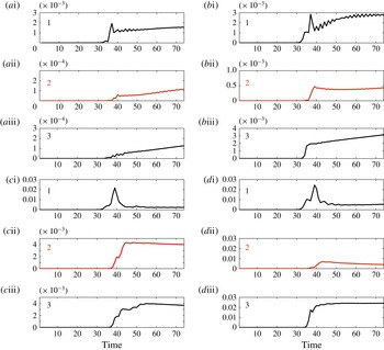
Figure 11. Mean-square error in an asymmetric channel. The number of the corresponding reach is displayed on the left of each graph. The channel in (ai–biii) has width
 $L=1$
; in (ci–diii) the channel has width
$L=1$
; in (ci–diii) the channel has width
 $L=3$
. For the first column the branching angle
$L=3$
. For the first column the branching angle
 ${\it\alpha}={\rm\pi}/6$
, while for the second column it is
${\it\alpha}={\rm\pi}/6$
, while for the second column it is
 ${\it\alpha}={\rm\pi}/3$
.
${\it\alpha}={\rm\pi}/3$
.
Shi et al. (Reference Shi, Teng and Sou2005) report laboratory experiments only for an asymmetric configuration with
 ${\it\alpha}={\rm\pi}/2$
. A range of channel widths are considered with
${\it\alpha}={\rm\pi}/2$
. A range of channel widths are considered with
 $L/{\it\lambda}_{e}\in [0.1,0.5]$
. Our case with
$L/{\it\lambda}_{e}\in [0.1,0.5]$
. Our case with
 $L=5$
is close to the upper bound of this interval. Their 2D Boussinesq simulations, in Cartesian coordinates, ‘were found to be in generally good agreement, especially for the transmitted waves’. Shi et al. (Reference Shi, Teng and Sou2005) also mention that ‘so far there have been a few numerical studies carried out to simulate solitary wave propagating through channel bends; however, these studies have not been verified by laboratory experiments’. The same holds for forked channels and solitary waves.
$L=5$
is close to the upper bound of this interval. Their 2D Boussinesq simulations, in Cartesian coordinates, ‘were found to be in generally good agreement, especially for the transmitted waves’. Shi et al. (Reference Shi, Teng and Sou2005) also mention that ‘so far there have been a few numerical studies carried out to simulate solitary wave propagating through channel bends; however, these studies have not been verified by laboratory experiments’. The same holds for forked channels and solitary waves.
We observed that for angles of about
 ${\it\alpha}={\rm\pi}/3$
the nonlinear compatibility condition was satisfactory for symmetric branching channels, but not so sharp for the asymmetric case. For angles of
${\it\alpha}={\rm\pi}/3$
the nonlinear compatibility condition was satisfactory for symmetric branching channels, but not so sharp for the asymmetric case. For angles of
 ${\it\alpha}={\rm\pi}/6$
both were fine. Therefore the following question arises: How does an asymmetric forked region depend on the value of the branching angle? In the book by Milne-Thomson (Reference Milne-Thomson1968) there is a streaming flow problem which is quite useful for addressing the point raised above. Consider the streaming potential flow depicted in figure 12. In Milne-Thomson (Reference Milne-Thomson1968) (§ 10.8, p. 289) the three channel reaches may have different widths. We have taken all widths equal to
${\it\alpha}={\rm\pi}/6$
both were fine. Therefore the following question arises: How does an asymmetric forked region depend on the value of the branching angle? In the book by Milne-Thomson (Reference Milne-Thomson1968) there is a streaming flow problem which is quite useful for addressing the point raised above. Consider the streaming potential flow depicted in figure 12. In Milne-Thomson (Reference Milne-Thomson1968) (§ 10.8, p. 289) the three channel reaches may have different widths. We have taken all widths equal to
 $L$
. Along the main reach the incoming uniform flow has a given speed equal to
$L$
. Along the main reach the incoming uniform flow has a given speed equal to
 $U_{1}$
. The goal is to find the limiting uniform flow speeds
$U_{1}$
. The goal is to find the limiting uniform flow speeds
 $U_{2}$
and
$U_{2}$
and
 $U_{3}$
in terms of the given data
$U_{3}$
in terms of the given data
 $U_{1}$
and
$U_{1}$
and
 ${\it\alpha}$
. This is equivalent to finding the limiting values of the Jacobian in our case. In light of this analogy, Milne-Thomson (Reference Milne-Thomson1968, equation (7), p. 292) yields
${\it\alpha}$
. This is equivalent to finding the limiting values of the Jacobian in our case. In light of this analogy, Milne-Thomson (Reference Milne-Thomson1968, equation (7), p. 292) yields
 $$\begin{eqnarray}\left(\frac{1}{|J|_{2}}\right)^{(1/2)-({\rm\pi}/2{\it\alpha})}-\left(\frac{1}{|J|_{3}}\right)^{(1/2)-({\rm\pi}/2{\it\alpha})}=1.\end{eqnarray}$$
It is convenient to denote
 ${\it\chi}\equiv |J|_{2}^{-1/2}$
and
${\it\chi}\equiv |J|_{2}^{-1/2}$
and
 $|J|_{3}=1/(1-|J|_{2}^{-1/2})^{2}$
, where
$|J|_{3}=1/(1-|J|_{2}^{-1/2})^{2}$
, where
 ${\it\chi}$
and
${\it\chi}$
and
 $(1-{\it\chi})$
are respectively the widths below and above the separatrix streamline that connects to the branching region’s inner corner as in figure 5. Equation (3.9) becomes
$(1-{\it\chi})$
are respectively the widths below and above the separatrix streamline that connects to the branching region’s inner corner as in figure 5. Equation (3.9) becomes
 $$\begin{eqnarray}{\it\chi}^{1-{\rm\pi}/{\it\alpha}}-(1-{\it\chi})^{1-{\rm\pi}/{\it\alpha}}=1.\end{eqnarray}$$
The roots can be computed and the corresponding asymptotic values of the Jacobian checked against numerical results produced by the Schwarz–Christoffel toolbox (Driscoll & Trefethen Reference Driscoll and Trefethen2002). The influence of the branching angle
 ${\it\alpha}$
on the Jacobian’s limiting (constant) value is highly nonlinear. For an angle of
${\it\alpha}$
on the Jacobian’s limiting (constant) value is highly nonlinear. For an angle of
 ${\it\alpha}={\rm\pi}/6$
there is no contrast between
${\it\alpha}={\rm\pi}/6$
there is no contrast between
 $|J|_{2}$
and
$|J|_{2}$
and
 $|J|_{3}$
, indicating no preferred reach for the transmitted wave. For an angle of
$|J|_{3}$
, indicating no preferred reach for the transmitted wave. For an angle of
 ${\it\alpha}={\rm\pi}/3$
we have that
${\it\alpha}={\rm\pi}/3$
we have that
 $|J|_{2}\approx 4.546244954163168$
and
$|J|_{2}\approx 4.546244954163168$
and
 $|J|_{3}\approx 3.546600469826436$
. The Jacobian is shown in figure 13. For these values the right-hand side of (3.9) is approximately 0.9996. The asymmetry is starting to play a role, as seen in the simulations.
$|J|_{3}\approx 3.546600469826436$
. The Jacobian is shown in figure 13. For these values the right-hand side of (3.9) is approximately 0.9996. The asymmetry is starting to play a role, as seen in the simulations.

Figure 12. The asymmetric branching region with the level curves of the conformal coordinate system
 ${\it\xi}-{\it\zeta}$
. These lines coincide with the equipotential levels of the velocity potential and the stream function (respectively), in the streaming flow problem presented in Milne-Thomson (Reference Milne-Thomson1968). The straight lines outside the flow domain indicate that the points at their extreme ends are mapped to the same position in the canonical domain.
${\it\xi}-{\it\zeta}$
. These lines coincide with the equipotential levels of the velocity potential and the stream function (respectively), in the streaming flow problem presented in Milne-Thomson (Reference Milne-Thomson1968). The straight lines outside the flow domain indicate that the points at their extreme ends are mapped to the same position in the canonical domain.

Figure 13. The Jacobian
 $|J|=|J|({\it\xi},{\it\zeta})$
for an asymmetric branching channel of width
$|J|=|J|({\it\xi},{\it\zeta})$
for an asymmetric branching channel of width
 $L=5$
. The secondary reach is at an angle of
$L=5$
. The secondary reach is at an angle of
 ${\it\alpha}={\rm\pi}/6$
(a) and at an angle of
${\it\alpha}={\rm\pi}/6$
(a) and at an angle of
 ${\it\alpha}={\rm\pi}/3$
(b), both in a configuration similar to figure 1.
${\it\alpha}={\rm\pi}/3$
(b), both in a configuration similar to figure 1.
To the best of our knowledge no wave model on a graph has these geometrical features systematically built into the equations, namely angles and asymmetry. For this reason the work by Jacovkis (Reference Jacovkis1991) and Bona & Cascaval (Reference Bona and Cascaval2008) should be considered as 1D valid approximations in the symmetric small-angle regime with
 $L_{1}=2L_{2}=2L_{3}$
.
$L_{1}=2L_{2}=2L_{3}$
.
The well-posedness of the present model is an open question. Our numerical simulations provide evidence and point in the direction of a well-posed system of PDEs defined in a non-standard (three-point graph-like) domain, a challenge for theoretical analysis. The following comments briefly illustrate the state of affairs.
Take the Boussinesq equations with either the linear compatibility conditions (3.3)–(3.4) or the nonlinear conditions (3.6)–(3.8). Approximate the Jacobian by its respective constant value given on each reach. Even in the constant coefficient regime (per reach), both cases define a new system of partial differential equations for which no existence and well-posedness analysis is available in the weakly nonlinear, weakly dispersive regime. Jacovkis (Reference Jacovkis1991) presented a well-posedness analysis in the subcritical linear hyperbolic regime, based on the method of characteristics. We should note that in the constant coefficient (
 $|J|\equiv 1$
) case our transversally averaged system reduces (on each reach) to the standard (depth-averaged) dimensionless Boussinesq system
$|J|\equiv 1$
) case our transversally averaged system reduces (on each reach) to the standard (depth-averaged) dimensionless Boussinesq system
 $$\begin{eqnarray}\displaystyle & \bar{{\it\eta}}_{t}+(1+\bar{{\it\eta}})\bar{u}_{{\it\xi}}+\bar{{\it\eta}}_{{\it\xi}}\bar{u}=0, & \displaystyle\end{eqnarray}$$
 $$\begin{eqnarray}\displaystyle & \displaystyle \bar{u}_{t}+\bar{{\it\eta}}_{{\it\xi}}+\frac{\bar{u}_{{\it\xi}}^{2}}{2}-\frac{\bar{u}_{{\it\xi}{\it\xi}t}}{3}=0. & \displaystyle\end{eqnarray}$$
 $$\begin{eqnarray}\displaystyle & \displaystyle \bar{{\it\eta}}_{t}+[(1+\bar{{\it\eta}})\bar{u}]_{{\it\xi}}+a\bar{u}_{{\it\xi}{\it\xi}{\it\xi}}-b\bar{{\it\eta}}_{{\it\xi}{\it\xi}t}=0, & \displaystyle\end{eqnarray}$$
 $$\begin{eqnarray}\displaystyle & \displaystyle \bar{u}_{t}+\bar{{\it\eta}}_{{\it\xi}}+\frac{\bar{u}_{{\it\xi}}^{2}}{2}+c\bar{{\it\eta}}_{{\it\xi}{\it\xi}{\it\xi}}-d\bar{u}_{{\it\xi}{\it\xi}t}=0, & \displaystyle\end{eqnarray}$$
 $u$
is evaluated. This choice changes the dispersion relation and therefore linear stability properties. The depth-averaged case above is equivalent to using the horizontal velocity at depth
$u$
is evaluated. This choice changes the dispersion relation and therefore linear stability properties. The depth-averaged case above is equivalent to using the horizontal velocity at depth
 $\sqrt{1/3}$
(Muñoz & Nachbin Reference Muñoz and Nachbin2006). For the bidirectional Boussinesq system the wave propagation direction is immaterial, and this is also the case in the forked region configuration.
$\sqrt{1/3}$
(Muñoz & Nachbin Reference Muñoz and Nachbin2006). For the bidirectional Boussinesq system the wave propagation direction is immaterial, and this is also the case in the forked region configuration.
For the variable coefficient case very little functional analysis and well-posedness theory is available for the initial value problem on the real line. For a specific variable-coefficient Boussinesq system on the real line an existence and well-posedness analysis is provided by Quintero & Muñoz (Reference Quintero and Muñoz2004), using the horizontal velocity evaluated at depth
 $\sqrt{2/3}$
, a particular case for which they were able to find an energy functional valid in the presence of highly disordered topographies.
$\sqrt{2/3}$
, a particular case for which they were able to find an energy functional valid in the presence of highly disordered topographies.
In the presence of boundary conditions, as for example the half-line, theory is very scarce. For bidirectional models Bona & Chen (Reference Bona and Chen1998) considered the boundary value problem for a specific (constant coefficient) Boussinesq system, where the horizontal velocity is evaluated at depth
 $\sqrt{2/3}$
. To the best of our knowledge no other bidirectional boundary value analysis is available in the literature. Bona, Chen & Saut (Reference Bona, Chen and Saut2004) present a class of Boussinesq systems which are (locally) nonlinearly well-posed, on the real line, in suitable function classes. The authors mention that a relevant theory is needed in the context where non-homogeneous boundary conditions are imposed at finite spatial portions of the domain. This type of analysis is available for some unidirectional models (such as Korteweg–de Vries) where the boundary value analysis is done on the half-line. Another example applies to the unidirectional BBM model on a graph as mentioned earlier (Bona & Cascaval Reference Bona and Cascaval2008). Articles on the functional analysis of boundary value problems and quarter-plane problems can be found in their references. These are for unidirectional wave models, and an example of a quarter-plane problem is the wave-maker problem for the BBM equation studied on the half-line. Bona & Fokas (Reference Bona and Fokas2008) describe open problems and present some relevant references on boundary value analysis for nonlinear waves. For bidirectional nonlinear waves in 1D forked domains there is only numerical evidence of well-behaved solitary wave solutions, namely the case presented here.
$\sqrt{2/3}$
. To the best of our knowledge no other bidirectional boundary value analysis is available in the literature. Bona, Chen & Saut (Reference Bona, Chen and Saut2004) present a class of Boussinesq systems which are (locally) nonlinearly well-posed, on the real line, in suitable function classes. The authors mention that a relevant theory is needed in the context where non-homogeneous boundary conditions are imposed at finite spatial portions of the domain. This type of analysis is available for some unidirectional models (such as Korteweg–de Vries) where the boundary value analysis is done on the half-line. Another example applies to the unidirectional BBM model on a graph as mentioned earlier (Bona & Cascaval Reference Bona and Cascaval2008). Articles on the functional analysis of boundary value problems and quarter-plane problems can be found in their references. These are for unidirectional wave models, and an example of a quarter-plane problem is the wave-maker problem for the BBM equation studied on the half-line. Bona & Fokas (Reference Bona and Fokas2008) describe open problems and present some relevant references on boundary value analysis for nonlinear waves. For bidirectional nonlinear waves in 1D forked domains there is only numerical evidence of well-behaved solitary wave solutions, namely the case presented here.
4. Conclusion
We have deduced a new model for solitary waves on a graph. For the first time a reduced 1D differential system of nonlinear wave equations is presented which contains information from the branching angles. New, more general and more accurate, nonlinear compatibility conditions are deduced at the branching region, which are shown to reduce to well-known compatibility conditions in a particular case. It has also been shown that angles of moderate values play a role in the reflection and transmission characteristics of solitary waves in branching channels. We have characterized the large angle regime where asymmetry starts to manifest itself through the Jacobian.
When comparing the reduced 1D model with the 2D ‘parent’ model, our results were accurate for a wide range of angles and channel widths. When the angles were greater than or equal to
 ${\it\alpha}={\rm\pi}/3$
the results started to deteriorate. Up to
${\it\alpha}={\rm\pi}/3$
the results started to deteriorate. Up to
 ${\it\alpha}={\rm\pi}/3$
the compatibility conditions satisfactorily handle the coefficient contrast (between reaches 2 and 3) that appears through the Jacobian. When this contrast further increases (with
${\it\alpha}={\rm\pi}/3$
the compatibility conditions satisfactorily handle the coefficient contrast (between reaches 2 and 3) that appears through the Jacobian. When this contrast further increases (with
 ${\it\alpha}$
), the flux across the separatrix, as indicated in figure 5, has to be incorporated into the compatibility conditions in some way. The correct form of this flux adjustment needs to be identified.
${\it\alpha}$
), the flux across the separatrix, as indicated in figure 5, has to be incorporated into the compatibility conditions in some way. The correct form of this flux adjustment needs to be identified.
The 1D reduced model was designed for long waves when these are compared to the channel width
 $L$
. The well-established linear compatibility condition was shown not to be accurate for a narrow channel of uniform width
$L$
. The well-established linear compatibility condition was shown not to be accurate for a narrow channel of uniform width
 $L=1$
even in the case of a small branching angle equal to
$L=1$
even in the case of a small branching angle equal to
 ${\it\alpha}={\rm\pi}/6$
. The solitary wave considered has an effective pulse width of
${\it\alpha}={\rm\pi}/6$
. The solitary wave considered has an effective pulse width of
 ${\it\lambda}_{e}\approx 13$
. For the narrow channel mentioned above, the small parameter, as indicated by Shi et al. (Reference Shi, Teng and Wu1998), is
${\it\lambda}_{e}\approx 13$
. For the narrow channel mentioned above, the small parameter, as indicated by Shi et al. (Reference Shi, Teng and Wu1998), is
 $L/{\it\lambda}_{e}\approx 0.08$
. For our wider channels we used
$L/{\it\lambda}_{e}\approx 0.08$
. For our wider channels we used
 $L=5$
, which leads to
$L=5$
, which leads to
 $L/{\it\lambda}_{e}\approx 0.4$
. Above this value the 1D results started to deteriorate. In the 2D numerical simulations of Shi et al. (Reference Shi, Teng and Sou2005), when
$L/{\it\lambda}_{e}\approx 0.4$
. Above this value the 1D results started to deteriorate. In the 2D numerical simulations of Shi et al. (Reference Shi, Teng and Sou2005), when
 $L/{\it\lambda}_{e}\approx 0.8$
the dynamics away from the forked region is shown to be 2D. The strong waveguide effect, as seen in figure 4, is no longer present. In this regime a 1D reduced model should not be expected to capture the effective dynamics accurately. Possibly when
$L/{\it\lambda}_{e}\approx 0.8$
the dynamics away from the forked region is shown to be 2D. The strong waveguide effect, as seen in figure 4, is no longer present. In this regime a 1D reduced model should not be expected to capture the effective dynamics accurately. Possibly when
 $L\leqslant 5$
, further improved compatibility conditions might be available for angles larger than
$L\leqslant 5$
, further improved compatibility conditions might be available for angles larger than
 ${\rm\pi}/3$
. We have not succeeded in finding this improved version.
${\rm\pi}/3$
. We have not succeeded in finding this improved version.
On this topic, several future problems are encouraged by the present results.
-
(a) Laboratory experiments dealing with angle diversity and its impact on the reflection–transmission problem, as well as approximate 1D regimes and its dependence on channel width. Some preliminary experimental results are reported by Shi et al. (Reference Shi, Teng and Sou2005).
-
(b) Mathematical analysis of the 2D model’s limiting behaviour as
$L/{\it\lambda}_{e}\rightarrow 0$
and the related impact of different compatibility conditions on 1D reduced models. Mathematical analysis is also needed to rigorously address the 1D problem on a tree-like domain with a Boussinesq-type system and nonlinear compatibility conditions. Nonlinear dispersive problems on the half-line are a theme of great current interest, as for example reported by Bona & Fokas (Reference Bona and Fokas2008). -
(c) To design further improved compatibility conditions, in particular for the asymmetric case with angle
${\it\alpha}>{\rm\pi}/3$
in channels of moderate width such as
$L=5$
.


Acknowledgements
The authors thank the referees for their valuable and constructive comments. The work of Nachbin was supported by CNPq grant 454027/2008-7 and by FAPERJ Cientistas do Nosso Estado grant 102917/2011. Part of this work was done while Nachbin was a David Parkin Visiting Professor at the Department of Mathematical Sciences, University of Bath, UK. The author is grateful to the University of Bath and to CAPES through ESN-4156-13-7. The work of Simões was supported by the Brazilian National Petroleum Agency (ANP) through the program COMPETRO PRH32. We are grateful to C. S. Ayala for his help regarding the numerical conformal mapping.
Appendix A. Numerical method
The 1D discretization follows the finite difference scheme used in the 2D simulations presented in Nachbin & Simões (Reference Nachbin and Simões2012). The major novelty in this presentation is the compatibility conditions and their implementation. Let
 $u_{j}^{n}=u({\it\xi}_{j},t^{n})$
, where
$u_{j}^{n}=u({\it\xi}_{j},t^{n})$
, where
 ${\it\xi}_{j}$
denotes mesh points with uniform spacing
${\it\xi}_{j}$
denotes mesh points with uniform spacing
 ${\rm\Delta}{\it\xi}$
. Centred finite differences are used and denoted by
${\rm\Delta}{\it\xi}$
. Centred finite differences are used and denoted by
 $du_{j}^{n}=(u_{j+1}^{n}-u_{j-1}^{n})/(2{\rm\Delta}{\it\xi})$
and
$du_{j}^{n}=(u_{j+1}^{n}-u_{j-1}^{n})/(2{\rm\Delta}{\it\xi})$
and
 $d^{2}u_{j}^{n}=(u_{j+1}^{n}-2u_{j}^{n}+u_{j-1}^{n})/{\rm\Delta}{\it\xi}^{2}$
. The 1D system (3.1)–(3.2) is rewritten in the form
$d^{2}u_{j}^{n}=(u_{j+1}^{n}-2u_{j}^{n}+u_{j-1}^{n})/{\rm\Delta}{\it\xi}^{2}$
. The 1D system (3.1)–(3.2) is rewritten in the form
 $$\begin{eqnarray}\displaystyle & \displaystyle \bar{{\it\eta}}_{t}=-\frac{1}{\overline{|J|}}[(1+\bar{{\it\eta}})\bar{u}_{{\it\xi}}+\bar{{\it\eta}}_{{\it\xi}}\bar{u}], & \displaystyle\end{eqnarray}$$
 $$\begin{eqnarray}\displaystyle & \displaystyle \left[\bar{u}-\left(\frac{\bar{u}_{{\it\xi}}}{3\overline{|J|}}\right)_{{\it\xi}}\right]_{t}=-\bar{{\it\eta}}_{{\it\xi}}-\left(\frac{\bar{u}^{2}}{2\overline{|J|}}\right)_{{\it\xi}}. & \displaystyle\end{eqnarray}$$
 $E_{j}^{n}$
, the right-hand side of (A 2) by
$E_{j}^{n}$
, the right-hand side of (A 2) by
 $G_{j}^{n}$
, and define an auxiliary function
$G_{j}^{n}$
, and define an auxiliary function
 $F\equiv \bar{u}-(\bar{u}_{{\it\xi}}/3\overline{|J|})_{{\it\xi}}$
seen in the left-hand side of (A 2). Using the centred difference schemes yields
$F\equiv \bar{u}-(\bar{u}_{{\it\xi}}/3\overline{|J|})_{{\it\xi}}$
seen in the left-hand side of (A 2). Using the centred difference schemes yields  $$\begin{eqnarray}\displaystyle & E_{j}^{n}=-1/\overline{|J|}_{j}[(1+\bar{{\it\eta}}_{j}^{n})~d\bar{u}_{j}^{n}+d\bar{{\it\eta}}_{j}^{n}\bar{u}_{j}^{n}], & \displaystyle\end{eqnarray}$$
 $$\begin{eqnarray}\displaystyle & G_{j}^{n}=-\bar{{\it\eta}}_{j}^{n}-d((\bar{u}_{j}^{n})^{2}/(2\overline{|J|}_{j})). & \displaystyle\end{eqnarray}$$
 $$\begin{eqnarray}\displaystyle \bar{{\it\eta}}_{j;0}^{n+1} & = & \displaystyle \bar{{\it\eta}}_{j}^{n}+{\rm\Delta}t~E_{j}^{n},\end{eqnarray}$$
 $$\begin{eqnarray}\displaystyle F_{j;0}^{n+1} & = & \displaystyle F_{j}^{n}+{\rm\Delta}t~G_{j}^{n}.\end{eqnarray}$$
 $$\begin{eqnarray}\displaystyle & \displaystyle \bar{{\it\eta}}_{j;{\it\mu}}^{n+1}=\bar{{\it\eta}}_{j}^{n}+\frac{{\rm\Delta}t}{2}[E_{j;{\it\mu}-1}^{n+1}+E_{j}^{n}], & \displaystyle\end{eqnarray}$$
 $$\begin{eqnarray}\displaystyle & \displaystyle F_{j;{\it\mu}}^{n+1}=F_{j}^{n}+\frac{{\rm\Delta}t}{2}[G_{j;{\it\mu}-1}^{n+1}+G_{j}^{n}]. & \displaystyle\end{eqnarray}$$
 ${\it\mu}=1,2,\dots ,M$
indicates the number of iterations/corrections made. The iterations are performed until a prescribed tolerance is reached. Usually in our simulations only two iterations were needed. A typical grid used has
${\it\mu}=1,2,\dots ,M$
indicates the number of iterations/corrections made. The iterations are performed until a prescribed tolerance is reached. Usually in our simulations only two iterations were needed. A typical grid used has
 ${\rm\Delta}{\it\xi}=0.05$
and
${\rm\Delta}{\it\xi}=0.05$
and
 ${\rm\Delta}t=0.025$
.
${\rm\Delta}t=0.025$
.
After each iteration the velocity vector
 $\bar{u}_{j;{\it\mu}}^{n+1}$
is recovered from the auxiliary function
$\bar{u}_{j;{\it\mu}}^{n+1}$
is recovered from the auxiliary function
 $F_{j;{\it\mu}}^{n+1}$
. This is needed in order to update
$F_{j;{\it\mu}}^{n+1}$
. This is needed in order to update
 $E_{j;{\it\mu}}^{n+1}$
and
$E_{j;{\it\mu}}^{n+1}$
and
 $G_{j;{\it\mu}}^{n+1}$
. This amounts to solving, at each stage, the discrete elliptic problem
$G_{j;{\it\mu}}^{n+1}$
. This amounts to solving, at each stage, the discrete elliptic problem
 $$\begin{eqnarray}\bar{u}_{j}^{n}-d(d\bar{u}_{j}^{n}/(3\overline{|J|}_{j}))=F_{j}^{n},\end{eqnarray}$$
with a known right-hand side and the corresponding boundary conditions for
 $\bar{u}$
, as will be described below. We are using a three-point centred scheme and therefore we have a sparse linear system of equations which is dealt with very efficiently in MATLAB, in particular performing the LU decomposition of the respective matrix at the beginning of a simulation, once and for all.
$\bar{u}$
, as will be described below. We are using a three-point centred scheme and therefore we have a sparse linear system of equations which is dealt with very efficiently in MATLAB, in particular performing the LU decomposition of the respective matrix at the beginning of a simulation, once and for all.


The implementation of the compatibility condition is the main difficulty in the 1D scheme. A solitary wave, as expressed in (2.3) and (2.4), travels through the main reach 1 towards the forked region. This travelling wave profile does not change until it gets close to the branching point.
In order to apply the compatibility condition we rewrite system (3.1)–(3.2) as a forced hyperbolic-like system, namely as
 $$\begin{eqnarray}\displaystyle & \displaystyle \bar{{\it\eta}}_{t}+\frac{1}{\overline{|J|}}[(1+\bar{{\it\eta}})\bar{u}_{{\it\xi}}+\bar{u}\bar{{\it\eta}}_{{\it\xi}}]=0, & \displaystyle\end{eqnarray}$$
 $$\begin{eqnarray}\displaystyle & \displaystyle \bar{u}_{t}+\left(\frac{\bar{u}}{\overline{|J|}}\right)\bar{u}_{{\it\xi}}+\bar{{\it\eta}}_{{\it\xi}}=\left(\frac{\bar{u}_{{\it\xi}}}{3\overline{|J|}}\right)_{{\it\xi}t}+\overline{|J|}_{{\it\xi}}\frac{\bar{u}^{2}}{2\overline{|J|}^{2}}. & \displaystyle\end{eqnarray}$$
 $C^{+}$
and
$C^{+}$
and
 $C^{-}$
while the underlying right and left (hyperbolic) propagating modes are
$C^{-}$
while the underlying right and left (hyperbolic) propagating modes are
 $A$
and
$A$
and
 $B$
respectively. Along the characteristic directions departing from each point
$B$
respectively. Along the characteristic directions departing from each point
 $p_{j}$
(depicted in figure 14), the above system of equations can be put into the form
$p_{j}$
(depicted in figure 14), the above system of equations can be put into the form  $$\begin{eqnarray}\displaystyle & \displaystyle \frac{D^{+}A}{Dt}=F_{1}(A,B), & \displaystyle\end{eqnarray}$$
 $$\begin{eqnarray}\displaystyle & \displaystyle \frac{D^{-}B}{Dt}=F_{2}(A,B). & \displaystyle\end{eqnarray}$$
 $p_{j}$
. The original variables of interest are recovered through expressions of the form
$p_{j}$
. The original variables of interest are recovered through expressions of the form
 $\bar{u}=G_{1}(A,B)$
and
$\bar{u}=G_{1}(A,B)$
and
 $\bar{{\it\eta}}=G_{2}(A,B)$
. For example, for the non-dispersive linear regime the formulas are quite simple. Let
$\bar{{\it\eta}}=G_{2}(A,B)$
. For example, for the non-dispersive linear regime the formulas are quite simple. Let
 $c=1/|J|$
where
$c=1/|J|$
where
 $A=\bar{u}+\bar{{\it\eta}}/c$
and
$A=\bar{u}+\bar{{\it\eta}}/c$
and
 $B=-\bar{u}+\bar{{\it\eta}}/c$
,
$B=-\bar{u}+\bar{{\it\eta}}/c$
,
 $G_{1}=(A-B)/2$
and
$G_{1}=(A-B)/2$
and
 $G_{2}=c(A+B)/2$
. This would be analogous to the case reported in Jacovkis (Reference Jacovkis1991) where all equations were linear including the compatibility conditions. Now we have nonlinear terms in each characteristic direction together with nonlinear compatibility conditions.
$G_{2}=c(A+B)/2$
. This would be analogous to the case reported in Jacovkis (Reference Jacovkis1991) where all equations were linear including the compatibility conditions. Now we have nonlinear terms in each characteristic direction together with nonlinear compatibility conditions.
Given the solution at time
 $t=t^{n}$
, the compatibility condition will provide updated boundary data at the points
$t=t^{n}$
, the compatibility condition will provide updated boundary data at the points
 $p_{j}$
, at the following time
$p_{j}$
, at the following time
 $t=t^{n+1}$
. This is performed in two steps, using the three points near the fork but not at the fork. Through the jump condition this allows for changes in wave height regarding reaches 2 and 3. With the corresponding upwind and downwind scheme for (A 12)–(A 13), compute
$t=t^{n+1}$
. This is performed in two steps, using the three points near the fork but not at the fork. Through the jump condition this allows for changes in wave height regarding reaches 2 and 3. With the corresponding upwind and downwind scheme for (A 12)–(A 13), compute
 $A_{p_{1}}^{n+1}$
,
$A_{p_{1}}^{n+1}$
,
 $B_{p_{2}}^{n+1}$
and
$B_{p_{2}}^{n+1}$
and
 $B_{p_{3}}^{n+1}$
as in the scheme depicted in figure 14. In this first step one computes the outgoing modes from each reach. For the second step rewrite the compatibility conditions in terms of the
$B_{p_{3}}^{n+1}$
as in the scheme depicted in figure 14. In this first step one computes the outgoing modes from each reach. For the second step rewrite the compatibility conditions in terms of the
 $A$
and
$A$
and
 $B$
modes. Having solved the first step we improved our compatibility system of three equations, now reduced to three unknowns. These unknowns are the incoming modes
$B$
modes. Having solved the first step we improved our compatibility system of three equations, now reduced to three unknowns. These unknowns are the incoming modes
 $B_{p_{1}}^{n+1}$
,
$B_{p_{1}}^{n+1}$
,
 $A_{p_{2}}^{n+1}$
,
$A_{p_{2}}^{n+1}$
,
 $A_{p_{3}}^{n+1}$
indicated by the dashed arrows. These incoming modes encode information from the nonlinear coupling of all three reaches via the compatibility conditions. We should point out that with the linear compatibility conditions (3.3)–(3.4) a resulting linear algebraic system arises for
$A_{p_{3}}^{n+1}$
indicated by the dashed arrows. These incoming modes encode information from the nonlinear coupling of all three reaches via the compatibility conditions. We should point out that with the linear compatibility conditions (3.3)–(3.4) a resulting linear algebraic system arises for
 $B_{p_{1}}^{n+1}$
,
$B_{p_{1}}^{n+1}$
,
 $A_{p_{2}}^{n+1}$
,
$A_{p_{2}}^{n+1}$
,
 $A_{p_{3}}^{n+1}$
. With the nonlinear compatibility conditions (3.6)–(3.8) a quadratic form
$A_{p_{3}}^{n+1}$
. With the nonlinear compatibility conditions (3.6)–(3.8) a quadratic form
 $\boldsymbol{H}(B_{p_{1}}^{n+1},A_{p_{2}}^{n+1},A_{p_{3}}^{n+1})=\boldsymbol{F}^{n+1}$
arises, which is solved by a Newton method. Using
$\boldsymbol{H}(B_{p_{1}}^{n+1},A_{p_{2}}^{n+1},A_{p_{3}}^{n+1})=\boldsymbol{F}^{n+1}$
arises, which is solved by a Newton method. Using
 $\bar{u}=G_{1}(A,B)$
and
$\bar{u}=G_{1}(A,B)$
and
 $\bar{{\it\eta}}=G_{2}(A,B)$
we obtain the corresponding updated (forked region) values
$\bar{{\it\eta}}=G_{2}(A,B)$
we obtain the corresponding updated (forked region) values
 $\bar{u}_{p_{j}}^{n+1}$
and
$\bar{u}_{p_{j}}^{n+1}$
and
 $\bar{{\it\eta}}_{p_{j}}^{n+1}$
,
$\bar{{\it\eta}}_{p_{j}}^{n+1}$
,
 $j=1,2,3$
. This is how the compatibility conditions force each reach through their extreme nodes
$j=1,2,3$
. This is how the compatibility conditions force each reach through their extreme nodes
 $p_{j}$
. For each reach, the inner-node update is now decoupled from the other reaches until the compatibility condition is again applied at the following time step. As an example, consider reach 1 and let
$p_{j}$
. For each reach, the inner-node update is now decoupled from the other reaches until the compatibility condition is again applied at the following time step. As an example, consider reach 1 and let
 $\boldsymbol{x}^{n}=[\bar{{\it\eta}}_{1}^{n},\bar{u}_{1}^{n},\dots ,\bar{{\it\eta}}_{j}^{n},\bar{u}_{j}^{n},\dots ,\bar{{\it\eta}}_{p_{1}-1}^{n},\bar{u}_{p_{1}-1}^{n}]$
store the inner nodes’ respective function values. In matrix notation the corrector scheme is given by
$\boldsymbol{x}^{n}=[\bar{{\it\eta}}_{1}^{n},\bar{u}_{1}^{n},\dots ,\bar{{\it\eta}}_{j}^{n},\bar{u}_{j}^{n},\dots ,\bar{{\it\eta}}_{p_{1}-1}^{n},\bar{u}_{p_{1}-1}^{n}]$
store the inner nodes’ respective function values. In matrix notation the corrector scheme is given by
 $\boldsymbol{x}_{{\it\mu}}^{n+1}=\unicode[STIX]{x1D648}_{E}\boldsymbol{x}^{n}+\unicode[STIX]{x1D648}_{I}\boldsymbol{x}_{{\it\mu}-1}^{n+1}+\boldsymbol{b}^{n+1}$
, where both the matrix
$\boldsymbol{x}_{{\it\mu}}^{n+1}=\unicode[STIX]{x1D648}_{E}\boldsymbol{x}^{n}+\unicode[STIX]{x1D648}_{I}\boldsymbol{x}_{{\it\mu}-1}^{n+1}+\boldsymbol{b}^{n+1}$
, where both the matrix
 $\unicode[STIX]{x1D648}_{E}$
for the explicit part and the matrix
$\unicode[STIX]{x1D648}_{E}$
for the explicit part and the matrix
 $\unicode[STIX]{x1D648}_{I}$
for the implicit part are tridiagonal. The known forcing term
$\unicode[STIX]{x1D648}_{I}$
for the implicit part are tridiagonal. The known forcing term
 $\boldsymbol{b}^{n+1}$
has information from the compatibility condition and the corresponding boundary conditions. Recall that the upwind/downwind schemes (at
$\boldsymbol{b}^{n+1}$
has information from the compatibility condition and the corresponding boundary conditions. Recall that the upwind/downwind schemes (at
 $p_{1}$
,
$p_{1}$
,
 $p_{2}$
and
$p_{2}$
and
 $p_{3}$
) together with the compatibility conditions produced the updated boundary values for
$p_{3}$
) together with the compatibility conditions produced the updated boundary values for
 $\bar{u}$
and
$\bar{u}$
and
 $\bar{{\it\eta}}$
at these points. The same type of matrix equation is used for the other two reaches. Obviously, for the predictor scheme there is only a matrix regarding the explicit part.
$\bar{{\it\eta}}$
at these points. The same type of matrix equation is used for the other two reaches. Obviously, for the predictor scheme there is only a matrix regarding the explicit part.
We summarize the main ideas used in the numerical strategy. Given the solution at time
 $t=t^{n}$
we impose the compatibility conditions (3.6)–(3.8) at the following discrete time
$t=t^{n}$
we impose the compatibility conditions (3.6)–(3.8) at the following discrete time
 $t=t^{n+1}$
. We rewrite these conditions using the right
$t=t^{n+1}$
. We rewrite these conditions using the right
 $A_{p_{j}}$
and the left
$A_{p_{j}}$
and the left
 $B_{p_{j}}$
(
$B_{p_{j}}$
(
 $j=1,2,3$
) propagating modes. There are six unknowns and three conditions. Three of these unknowns (namely the out-propagating modes relative to each reach) are approximated by the method of characteristics via (A 12)–(A 13). These are the solid arrows in figure 14. Then the remaining three incoming modes (dashed arrows) are computed by the three (quadratic) compatibility conditions. Their values produce updated boundary data (
$j=1,2,3$
) propagating modes. There are six unknowns and three conditions. Three of these unknowns (namely the out-propagating modes relative to each reach) are approximated by the method of characteristics via (A 12)–(A 13). These are the solid arrows in figure 14. Then the remaining three incoming modes (dashed arrows) are computed by the three (quadratic) compatibility conditions. Their values produce updated boundary data (
 $\bar{u}_{p_{j}}^{n+1},\bar{{\it\eta}}_{p_{j}}^{n+1}$
) at the forked region nodes for the corresponding reach. At the other extreme of the reach homogeneous Dirichlet data are used. At this stage the predictor–corrector scheme can be used to evolve the solution values within each reach.
$\bar{u}_{p_{j}}^{n+1},\bar{{\it\eta}}_{p_{j}}^{n+1}$
) at the forked region nodes for the corresponding reach. At the other extreme of the reach homogeneous Dirichlet data are used. At this stage the predictor–corrector scheme can be used to evolve the solution values within each reach.


