Calculation of array factor of a planar array with multiple beams in two dimensions

In this sub-section, a planar array, which can generate multiple beams in two dimensions (x and y directions) has been synthesized. In [Reference Chou11], a planar array with multiple beams in one dimension (x direction) was analyzed. The array plane is coincident with the x–y plane as illustrated in Fig. 1. Decomposition of an array into interleaved sub-arrays eliminates the grating lobes in the visible region. In [Reference Chou11], a planar array with interleaved sub-arrays in each row (x direction) was analyzed. The array factor in this sub-section is different from the array factor in [Reference Chou11] due to the interleaved sub-arrays in two dimensions. Figure 2 shows an arbitrary row of an array with interleaved sub-arrays and lateral elements (skirt elements).

Fig. 1. Model of a planar array with multiple beams in two dimensions.

Fig. 2. Sample row of an array with interleaved sub-arrays and skirt elements.

The α _x and α _y are the parameters, which depend on the beam indexes in the x and y directions (α _xi and α _yi), respectively. These parameters can be calculated using (3) and (4). In this design, the origin of coordinate system is assumed in the middle of the beams and the number of beams is even. The beam index in the x direction (α _xi) varies in the range of 1 to P _x. Similarly, α _yi varies between 1 and P _y. Figure 3 shows α _x for eight beams in the x direction.

(3)$$\alpha _x = \alpha _{xi}-( P_x + 1) /2{\rm \;\;\;\;\;\;\;}$$

(4)$$\alpha _y = \alpha _{yi}-( P_y + 1) /2$$

Fig. 3. α_x, α_xi, and r_x for P_x = 8 and N_x = 2.

Using (1) and (3), the main beam peak locations in the x direction (θ _αx) for each α _xi can be obtained as follows:

(5)$$\sin ( {\theta_{\alpha x}} ) = \alpha _{x \;}\Delta \sin \theta _{\,peak_x} = ( {-P_x/2-0.5 + \alpha_{xi}} ) ( {\lambda /P_xN_{sx}d_x} ) $$

In a similar manner, the main beam peak locations in the y direction (θ _αy) can be attained. The calculated main beam peak locations have been used in the calculation of array factor. The array factor of a planar array in the x–y plane with interleaved sub-arrays in both x and y directions is expressed in (6). This array can generate multiple beams in two dimensions.

(6)$$AF = \mathop \sum \limits_{a = 1}^{N_{sx}} AF_{subx}( a) e^{i\psi ( {\alpha_{xi}, a} ) + 2\pi i( {a-1} ) d_xu/\lambda } \times \mathop \sum \limits_{b = 1}^{N_{sy}} AF_{sub_y}( b) e^{i\psi ( {\alpha_{yi}, b} ) + 2\pi i( {b-1} ) d_yv/\lambda }$$

where u = sinθ cos φ and v = sinθ sin φ. As depicted in Fig. 2, the core array consists of the interleaved sub-arrays. Each sub-array is excited with a different BFN. The phase differences ψ(α _xi, a) and ψ(α _yi, b) should be added to the input ports of each BFN in the x and y directions, respectively. AF _subx(a) and $AF_{sub_y}( b)$ are the array factors of each sub-array in the x and y directions, respectively. The phase of elements in each sub-array is adjusted for creating orthogonal beams. The indexes of the sub-arrays in the x and y directions are denoted by letters a and b, respectively.

The AF _subx(a) is calculated using (7). q _x is the element index in each sub-array in the x direction, and vary from 1 to N _x. N _x and N _y are the number of elements in each sub-array in the x and y directions, respectively. q _x is shown in Fig. 2. B _x(q _x) is the excitation amplitude of $q_x^{th}$ element of a ^th sub-array in each row, and B _y(q _y) is the excitation amplitude of $q_y^{th}$ element of b ^th sub-array in each column. AF _suby (b) can be obtained in a similar manner by replacing q _x, N _sx, N _x, u, α _x, and B _x(q _x) in (7) with q _y, N _sy, N _y, v, α _y, and B _y(q _y), respectively.

(7)$$AF_{sub_x}( a) = \mathop \sum \limits_{q_x = 1}^{N_x} B_x( q_x) e^{-( ( 2\pi i\alpha _x( q_x-1) ) /P_x) + 2\pi i( {q_x-1} ) N_{sx}d_xu/\lambda }$$

ψ(α _xi, a) depends on the beam index (α _xi) and the sub-array index (a) in the x direction. This phase difference has been calculated using (8) [Reference Chou11]:

(8)$$\psi ( {\alpha_{xi}, \;a} ) = -2\pi ( {a-1} ) d_x\sin ( {\theta_{\alpha x}} ) /\lambda $$

In a similar manner, ψ(α _yi, b) can be obtained for the y direction.

Calculating phases of the lateral elements

As described in the section “Array aperture size reduction,” non-uniform amplitude distribution of an array decreases the aperture efficiency, but it may improve the other radiation parameters of the array. Consequently, the choice of the proper amplitude distribution is a trade-off between the aperture size and the antenna pattern requirements.

One of the techniques to narrow the beam-width and to reduce the SLLs in a multiple beam array with interleaved sub-arrays is the addition of some lateral elements (skirt elements) to the right and left margins of the core array [Reference Chou11]. This technique may improve the carrier to interference ratio and has been adopted in our design. Numbers of right and left skirt elements in the x direction are N_skrx and N_sklx, correspondingly, and they are equal to N _skx/2. Similarly, N _skry = N _sky/2 and N _skly = N _sky/2 are the numbers of right and left skirt elements in the y direction. N _skx and N _sky are the total number of skirt elements in each row and column, respectively. The overall number of elements in each row of the core array is shown with N _tx and is equal to N _sxN _x. Also, N _ty is the total number of elements in each column of the core array and is equal to N _syN _y.

Figure 4 illustrates one row of an array with P _x = 8, N _x = 2, N _sx = 18, and N _skx = 8 that consists of some core and skirt elements. For each skirt element, a power divider is needed. As illustrated in Fig. 4, for the right skirt elements, each power divider splits the input power between the k^th left core element and the k^th right skirt element (embedded in BFN1s). The value of k varies from 1 to N _skrx in the x direction and from 1 to N _skry in the y direction. As a result, in the x direction, the amplitude coefficient of the k ^th right skirt element (A _skrx(k)) and the corresponding left core element (A _x(k)) are related as expressed in (9). Similar relation exists between the k ^th right skirt element (A _skry(k)) and the corresponding left core element (A _y(k)) in the y direction.

(9)$$A_x( k ) ^2 + A_{skrx}( k ) ^2 = 1{\rm \;\;\;\;}$$

Fig. 4. Designed array configuration for each row of the planar array (P _x = 8, N _sx = 18, N _x = 2, N _skx = 8).

To keep the peak locations of the beams, extra phase shifts $( \Delta \varphi _{x\_right})$ must be added to the right skirt elements. This extra phase shift arises from the difference in the distance between the k ^th core element and the k ^th right skirt element. The extra phase shift $( \Delta \varphi _{x\_right})$ for the beam with a peak location of θ _αx is expressed in (10) using (5):

(10)$$\Delta \varphi _{x\_right} = \displaystyle{{-2\pi N_{tx}d_x\sin ( \theta _{\alpha x}) } \over \lambda } = \displaystyle{{-2\pi N_x( {\alpha_{xi}-0.5P_x-0.5} ) } \over {P_x}}$$

In [Reference Chou11], the number of beams (P _x) and the number of sub-array elements (N _x) have been assumed to be equal, and the needed extra phase shift has been obtained using this assumption.

In this paper, it has been assumed that P _x and N _x are in general unequal. The amount of phase difference in (10) depends on the ratio P _x to N _x (M _x = P _x/N _x) as presented in (11):

(11)$$\Delta \varphi _{x\_right} = \left\{{\matrix{ {( {-2\alpha_{xi} + 1} ) \displaystyle{\pi \over {M_x}}; \;\quad \quad N_x\,\colon\, even} \cr {( {-2\alpha_{xi} + 1 + M_x} ) \displaystyle{\pi \over {M_x}}; \;\;\;N_x\,\colon\, odd} \cr } } \right.$$

Therefore, $\Delta \varphi _{x\_right}\;$ depends on the beam index (α _xi), and under the condition of M _x ≠ 1 varies for different beams. The previously mentioned condition implies different numbers of beam ports and elements in each sub-array. It can be deduced from (11) that for even values of N _x there are M _x discrete phases, which must be applied to the skirt elements for various beams. As a result, the total beams in each row can be divided into M _x beam groups (BG). For each BG, the same $\Delta \varphi _{x\_right}\;$must be added to the right skirt elements.

In Fig. 3, BGs of an array with P _x = 8 and N _x = 2 have been indicated. In each row, the index of BGs is shown with c _x and varies between 1 and M _x. In the same way, as illustrated in Fig. 4, the power dividers used in the left skirt elements (devised in BFN2s) split the input power between the m ^th left skirt element and N _tx − N _sklx + m ^th core element. The amplitude coefficients of the left skirt elements and the corresponding core elements in the x direction must satisfy (12). In a similar manner, the amplitude coefficient of the m ^th left skirt element (A _skly(m)) and N _ty − N _skly + m ^th core element (A _y(N _ty − N _skly + m)) in each column are related.

(12)$$A_x( {N_{tx}-N_{sklx} + m \;} ) ^2 + A_{sklx}( m ) ^2 = 1$$

Similar to the right skirt elements, the extra phase shifts which must be added to the left skirt elements in each row can be calculated by using (13):

(13)$$\Delta \varphi _{x\_left} = \left\{{\matrix{ {( {2\alpha_{xi}-1} ) \displaystyle{\pi \over {M_x}}; \;\;\;\;\;\;\;\;\;\;\;\;\;\;N_x\,\colon\, even} \cr {( {2\alpha_{xi}-1-M_x} ) \displaystyle{\pi \over {M_x}}; \;\;\;N_x\,\colon\, odd} \cr } } \right.$$

Similarly, the total beams in each column should be divided into M _y BGs (M _y = P _y/N _y). The corresponding index is indicated by c _y, and has a value between 1 and M _y.

The extra phase shifts, which must be added to the right and left skirt elements in each column $( \Delta \varphi _{y\_right}, \;\,\varphi _{y\_left})$ can be calculated similarly using (11) and (13).

Devising the BFN

In [Reference Chou11], regarding equal numbers of beams and sub-array elements in each row and column, the BFN consisted of several BMs as sub-array beam-forming networks (SABFNs). Devised BFN in this paper consists of three types of SABFNs that can create orthogonal beams, and are denoted BFN1, BFN2, and BFN3 blocks in Fig. 4. Each sub-array is excited with one of the previously mentioned SABFNs.

In contrast to the BFN in [Reference Chou11], the proposed SABFN in this paper exhibits different numbers of beam ports and sub-array ports, and it has the ability of adding different phase shifts to different BG signals for excitation of skirt elements.

In each row, the first type SABFN (BFN1) is designed for feeding the right skirt elements and the first N _skrx core elements. Consequently, it has P _x input ports and N _x + 1 array ports. In the second type SABFN which feeds each row (BFN2), there are P _x input ports and N _x + 1 array ports. It has been designed for feeding the left skirt elements and the last N _sklx core elements. The third type SABFN (BFN3) has been designed for feeding the other core elements. Therefore, it has P _x input ports and N _x array ports. As shown in Fig. 4, some N _sx − way equal power dividers are embedded for distributing input powers between the sub-arrays. The number of these power dividers in each row is P _x.

Similar SABFNs are needed for excitation of the sub-arrays in each column: BFN1 and BFN2 with P _y input ports and N _y + 1 array ports, and BFN3 with P _y input ports and N _y array ports.

In each row, the excitation signals of the array elements, which are fed by BFN1 block can be obtained from (14). The excitation signal of the $q_x^{th}$ element of a ^th sub-array is denoted by $E_{q_x}( a)$. In (14), A _x(a) is the amplitude coefficient of a ^th sub-array, and $V_{\alpha _{xi}\;}$ is the corresponding voltage at the $\alpha _{xi}^{th}$ beam which excites the BFN1.

(14)$$E_{q_x}( a) = \displaystyle{{A_x( a) \over \sqrt {N_x} }}\mathop \sum \limits_{\alpha _{xi} = 1}^{P_x} \;V_{\alpha _{xi} \;}e^{( -2\pi i( {q_x-1} ) ( {\alpha_{xi}-( ( P_x + 1) /2) } ) ) /P_x}$$

The signals, which are relevant to different BGs feed the right skirt elements with different phase shifts, as denoted in (11). Therefore, the signals which are relevant to different BGs should be separated. As a result, $E_{q_x}( a)$ can be re-written in the form of M _x separated signals as shown in (15), which holds under the condition of N _skrx < N _sx:

(15)$$\eqalign{& E_{q_x}( a) = \mathop \sum \limits_{c_x = 1}^{M_x} E_{q_x}^{c_x} \cr& = \displaystyle{{A_x( a) } \over {\sqrt {N_x} }}\mathop \sum \limits_{c_x = 1}^{M_x} {\kern 1pt} \mathop \sum \limits_{r_x = 1}^{N_x} {\kern 1pt} V_{c_x + ( {r_x-1} ) M_x \;}e^{( -2\pi i( {q_x-1} ) ( {c_x + ( {r_x-1} ) M_x- \;( ( P_x + 1) /2) } ) ) /P_x}}$$

where $E_{q_x}^{c_x} \;$ is the component of $E_{q_x}( a) .{\rm \;\;}$ In (15), r _x is a parameter that points to the index of the beam in each BG of each row. The r _x parameter varies between 1 and N _x, and is obtained using (16):

(16)$$r_x = \displaystyle{{\alpha _{xi}-c_x} \over {M_x}} + 1$$

In Fig. 3 the relation between r _x and α _xi has been illustrated for P _x = 8, N _x = 2. Also, in each column, r _y parameter is defined for pointing to the index of the beams in each BG.

In each row, the excitation signal of a ^th right skirt element is denoted by E _skrx(a) and since q _x = 1 (right skirt elements are fed by first sub-array elements), it can be obtained using (17):

(17)$$E_{skrx}( a) = \mathop \sum \limits_{c_x = 1}^{M_x} E_{skrx}^{c_x} = \displaystyle{{A_{skrx}( a) } \over {\sqrt {N_x} }}\mathop \sum \limits_{c_x = 1}^{M_x} e^{i\Delta \varphi _{x\_right}( {c_x} ) }\mathop \sum \limits_{r_x = 1}^{N_x} V_{c_x + ( {r_x-1} ) M_x \;}$$

Since in BFN1, the input power of each beam is divided between core elements and right skirt elements, A _skrx(a) and A _x(a) are the amplitude coefficients that must satisfy (9). Thus, BFN1s that excite different sub-arrays may have unequal two-way power dividers (Dividing ratio 1 = A _skrx(a)/A _x(a)). A _x(a) equals 1 for q _x > 1.

Devised BFN in this paper can be realized by conventional microwave circuits. In Fig. 5, the main parts of BFN1 based on (15) and (17) are illustrated. As can be inferred, for each BG, separate N _x × N _x inner BFNs have been embedded. In addition, for excitation of the skirt element, different phase shifts have been added to the signals from various BGs.

Fig. 5. BFN1 block.

The relation between input and output signals of each N _x × N _x inner BFN is presented in (18):

(18)$$\eqalign{P_{q_x}^{c_x} & = e^{i\pi ( {q_x-1} ) }( {V_{c_x\;} + V_{c_x + M_x\;}e^{-2\pi i( {q_x-1} ) /N_x} }\cr& + \cdots + V_{c_x + ( {N_x-1} ) M_x\;}e^{-( 2\pi i( {q_x-1} ) ( {N_x-1} ) ) /N_x })} $$

Accordingly, for N _x = 2, the inner BFN becomes a 180° hybrid. For N_x = 4, the inner BFN is realized by four 180° hybrids, as depicted in Fig. 6.

Fig. 6. 4 × 4 inner BFN.

Similarly, for the array elements, which are excited by BFN2 block, the excitation signal of the $q_x^{th}$ element of a ^th sub-array $( E_{q_x}( a) )$and m ^th left skirt element ((E _sklx(m))) can be derived using (19) and (20). Here, a is equal to N _tx − N _sklx + m. In (19) and (20), A _sklx(m) and A _x(N _tx − N _sklx + m) must satisfy (12). Since the left skirt elements are fed by the last elements of the sub-arrays in the core, A _x(N _tx − N _sklx + m) equals 1 for q _x < N _x.

(19)$$\eqalign{E_{q_x}( a ) & = \mathop \sum \limits_{c = 1}^{M_x} E_{q_x}^{c_x} = \displaystyle{{A_x( {N_{tx}-N_{sklx} + m} ) \over \sqrt {N_x} }} \cr& \mathop \sum \limits_{c_x = 1}^{M_x} \mathop \sum \limits_{r_x = 1}^{N_x} V_{\alpha _{xi}}e^{( -2\pi i( {q_x-1} ) ( {c_x + ( {r_x-1} ) M_x- \;( ( P_x + 1) /2) } ) ) /P_x}}$$

(20)$$E_{sklx}( m) = \mathop \sum \limits_{c_x = 1}^{M_x} E_{skl}^{c_x} = \displaystyle{{A_{sklx}( m) \over \sqrt {N_x} }}\mathop \sum \limits_{c_x = 1}^{M_x} e^{i\Delta \varphi x\_{left}( {c_x} ) }\mathop \sum \limits_{r_x = 1}^{N_x} V_{\alpha _{xi} \;}{\rm \;\;}$$

where $E_{q_x}^{c_x} \;$and $E_{skl}^{c_x}$ are the components of $E_{q_x}( a)$ and E _sklx(m), respectively. Similar to BFN1, BFN2s that feed different sub-arrays may be different in the dividing ratios of their power dividers (Dividing ratio 2 = A _sklx(m)/A _x(a)). The block diagram of BFN2 is illustrated in Fig. 7.

Fig. 7. BFN2 block.

Finally, excitation signal of the $q_x^{th}$ element of each sub-array, which is excited by BFN3, can be calculated as follows:

(21)$$E_{q_x} = \displaystyle{1 \over {\sqrt {N_x} }}\mathop \sum \limits_{a = 1}^{P_x} V_{\alpha _{xi}}e^{( -2\pi i( {q_x-1} ) ( {\alpha_{xi}- \;( ( P_x + 1) /2) } ) ) /P_x}$$

The excitation signals of the sub-array elements in each column $( E_{q_y}) \;$can be calculated in a similar manner, and their corresponding relations have not been repeated here.

Antenna requirements regarding sub-beam concept

Technical requirements of an antenna force the designer to select the antenna type and proper techniques to implement the antenna and feeding network. The requirements of a satellite antenna are derived from the conceptual design of the satellite payload. Satellite system specifications which are obtained from mission definition and analysis are the input parameters for the conceptual design of the payload [Reference Larson and Wertz14].

The main requirements of the multiple beam antenna, which can provide a frequency re-use factor of 4 for a high-throughput GEO satellite, are listed in Table 1. In this table, θ _dx and θ _dy are the angular distances between peak points of the adjacent beams in the x and y directions, and θ ₀ is the spot beam width. Total number of spots in the coverage domain is 16 and their beam width is 1°. These parameters are shown in Fig. 8. Since the cells in the coverage area are hexagonal, the angular distance between spot beams in the x and y directions can be calculated as:$\;\theta _{dx} = \sqrt 3 \theta _0/2 = 0.86^\circ$, and θ _dy = 0.75 θ ₀ = 0.75°. In Table 1, G _EOC is the minimum required gain for antenna at the EOC in the case of maximum scan angle. The contour level of spot beams has been selected to be 4 dB. It means that the antenna should be designed for multiple beams with peak gains of 46 dBi.

Fig. 8. Spot beam and sub-beam configuration.

Table 1. Requirements of a conventional multi-beam antenna and a multi-beam antenna using sub-beam concept (sub-beam cluster size = 4)

As described in the section “Array aperture size reduction,” by dividing each spot beam into several sub-beams, the peak gains of the antenna beams can be decreased. Consequently, the array aperture size can be reduced considerably. Increasing the number of sub-beams in each spot reduces the sub-beam peak gain; and therefore, decreases the antenna aperture size. On the other hand, increasing the sub-beam cluster-size increases the total number of sub-beams in the antenna system and the BFN complexity enhances. For this reason, an intermediate number for the sub-beam cluster size is used (sub-beam cluster size is 4). The configuration of the spot beams and sub-beams for a specified coverage domain is illustrated in Fig. 8. Sub-beams are equally spaced in the x and y directions and the angular distances between adjacent sub-beams in the x and y directions are θ _dsx = θ _dx/2 = 0.43° and θ _dsy = θ _dy/2 = 0.375°, respectively.

Regarding the sub-beam cluster size (which is equal to 4), the contour level of multiple spot beams (4 dB), and the analysis results in [Reference Kilic and Zaghloul3], the required contour level of the sub-beams becomes 1 dB. Therefore, the antenna should provide multiple sub-beams with peak gains of 43 dBi. The design requirements of the antenna with multiple sub-beams are presented in Table 1.

Array optimization concerning sub-beam concept

Using the relations presented in previous sections, a planar array of circular patches has been designed. In addition, the corresponding directivity patterns for the planar array have been calculated. The directivity pattern of the array element versus θ at an operating frequency of 3.64 GHz is depicted in Fig. 9. In this design, the circular patches have a radius of 1.24 cm. The substrate is an RO4003 with a thickness and dielectric constant of 0.8 mm and 3.55, respectively.

Fig. 9. Directivity pattern of the circular patch as the array element.

The peak locations of all sub-beams are depicted in Fig. 10. Each sub-beam has been specified with a number. Furthermore, contours of all main spots have been illustrated with different color circles. Circles that are similar in color are co-channel spots and operate in the same frequency bands and have the same polarizations. The operating frequency band is 3600–3680 MHz and is divided into two sub-bands: 3600–3640 and 3640–3680 MHz. Each sub-band is intended for two orthogonal linear polarizations. Green and blue circles have been used for vertical polarization, while red and purple circles have been used for horizontal polarization.

Fig. 10. Peak locations of all sub-beams and contours of the main spots.

As mentioned in (6), each sub-beam pattern depends on α _xi and α _yi and the selection of these two parameters depends on the sub-beam location. For example, as illustrated in Fig. 10, in the sub-beams 19 and 27, α _xi is 3, and α _yi takes the values 3 and 4, respectively. Also, in the sub-beams 20 and 28, α _xi is 4 and α _yi takes values 3 and 4, respectively.

To calculate the patterns of sub-beams 1–16, and 33–48, which are asymmetrical with respect to the y coordinate axis, some amount of phase shifts must be added to the excitation signals of the related beam ports.

The carrier to interference ratio (C/I) is a figure of merit for multi-beam arrays and determines the amount of interference of co-channel spots in each spot. To calculate C/I, the location of a specified spot should be extracted. In this way, in each constant φ plane, the range of elevation angles (θ) which are located in the specified spot will be calculated. As all of these coordinates (φ, θ) are located in a spot, the carrier and interfering signal in each coordinate should be calculated.

For example, the carrier magnitude in spot 6 is a linear combination of sub-beams 19, 20, 27, and 28. The co-channel interference in this spot is made of sub-beams 23, 24, 31, 32, 49, 50, 57, 58, 53, 54, 61, and 62, which are linearly added together. By this method, the desired C/I in all points of the desired spot can be achieved.

The parameters which should be determined in the array design process are N _sx, N _x, N _skx, A _sklx, A _skrx, d _x, N _sy, N _y, N _sky, A _skly, A _skry, and d _y.

Regarding (1) and the requirements which are listed in Table 1 for the multiple sub-beam antenna, N _sxd _x/λ and N _syd _y/λ take the values 16.65 and 19.09, respectively.

Calculating the antenna parameters by an iteration method subject to the previously mentioned conditions is very time consuming. In this paper, the GA has been used as an optimization method in the array design. In the GA, solutions are individuals of a population which change from one generation to the next generation. Each individual consists of several genes, which are parameters of the problem. Parents can be selected stochastically with a strategy like roulette-wheel method. In each generation, gene mutation is an activity, which avoids convergence to local extremes. As a result, the GA optimization converges to the global solution and stays away from local extremes. Details about the GA and its related parameters were presented in [Reference SharifiMoghaddam15–Reference Haupt and Haupt18].

The parameters in the GA optimization are selected in a manner that best solutions are achieved in the shortest time. In the present optimization, the population size, the probability of crossover, the probability of mutation and overlap are 20, 0.8, 0.07, and 50%, respectively.

The cost function is given in (22). In this expression, G _g and (C/I) _g are the goals that should be reached by G _EOC and (C/I) _min, respectively. The w1 and w2 are optimization weights, which take values corresponding to the importance of the previously mentioned parameters, and here they are taken to be 1. The (C/I)_min is the minimum amount of C/I in the spot region.

(22)$$cost = w1\vert {G_{EOC}-G_g} \vert + w2\left[{{\left({\displaystyle{C \over I}} \right)}_g-{\left({\displaystyle{C \over I}} \right)}_{min}} \right]$$

The starting point for optimization is the first estimation of the designer for the array parameter. At the beginning of the optimization process, d _x and d _y were nearly equal to half-wavelength. In addition, N _sx and N _sy have been chosen to satisfy N _sxd _x/λ = 16.65 and N _syd _y/λ = 19.09. The N _x, N _y, N _skx, and N _sky have been roughly estimated with the required array gain (given in the third column of Table 1). Therefore, the initial values for the optimization process were N _sx = 33, d _x = 0.5045λ,N _x = 2, N _skx = 2, A _sklx = 0.6, A _skrx = 0.6, N _sy = 38, d _y = 0.5024λ, N _y = 2, N _sky = 2, A _skly = 0.6, and A _skry = 0.6. The cost function at the starting point was 1.9371. With the aid of the GA, the cost function has been reduced to −0.3886. The final array parameters are listed in the third column of Table 2. After optimization, the (C/I) _min has been improved by 2.569 dB.

Table 2. Optimization results of a conventional multiple beam antenna and the optimized multiple sub-beam antenna (sub-beam cluster size = 4)

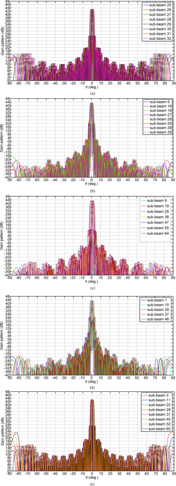
The gain patterns of the optimized multiple sub-beam array in the φ = 0°, φ = 22°, φ = 45°, φ = 67°, and φ = 90° constant planes are illustrated in Figs 11(a), (b), (c), (d), and (e), correspondingly. As illustrated in these figures, grating lobes have been eliminated in the visible region. It has been assumed that the coordinate origin is located at the center of sub-beam 28 (refer to Fig. 10). In Fig. 12, the sub-beams in the φ = 0° constant plane for the θ between −10° and 10° are presented. As can be inferred, the corresponding values of G _EOC and crossover level are 42 dBi and 1 dB, respectively. The angular distance between the adjacent beams in the x direction agrees with the antenna requirements in Table 1 (third column). In this array, SLL has been decreased to −16 dB, which is lower compared to the value of −13 dB observed in the uniform excitation. This SLL improvement is the result of adding skirt elements and optimum non-uniform amplitude distribution.

Fig. 11. Optimization results of the multiple sub-beam antenna, gain patterns versus θ in the: (a) φ = 0°, (b) φ = 22°, (c) φ = 45°, (d) φ = 67°, and (e) φ = 90° constant planes.

Fig. 12. Gain patterns of the multiple sub-beam antenna versus θ in φ = 0° constant plane.

C/I versus θ in different φ planes of the desired spot are illustrated in Fig. 13. As depicted in this figure, the minimum amount of C/I in the spot domain is more than 8.5 dB and satisfies the requirement listed in Table 1. Three-dimensional (3D) gain pattern of the synthesized multiple sub-beam array is illustrated in Fig. 14. Design of a proper BFN for the optimized array antenna will be described in the section “Designing the block diagrams of BFN for multiple sub-beam array.”

Fig. 13. C/I (dB) in the domain of spot 6.

Fig. 14. 3D gain pattern of the designed multiple sub-beam antenna (in dB).

Comparing a multiple sub-beam antenna with a conventional multiple beam antenna

In this sub-section, an array with conventional requirements of a multiple beam antenna (refer to Table 1) has been designed and optimized by means of the GA. The aim of this design is the array aperture size reduction using sub-beam concept. The results after GA optimization are listed in Table 2. The consequence is 36.7% reduction in aperture size and elements in the multiple sub-beam antenna. Figure 15(a) shows directivity pattern of the beams, which are located in the diagonal axis plane of the spots. Figure 15(b) illustrates C/I for different constant φ planes in spot 6. In this design, the coordinate origin has been located at the center of spot 6.

Fig. 15. Optimization results of the multiple beam antenna: (a) gain patterns in the diagonal plane crossing beams 1, 6, 11, and 15 and (b) C/I (dB) in the domain of spot 6.

Full-wave simulation

The full-wave simulation resembles the radiation characteristics of an array in the praxis. For this reason, the planar array has been simulated in Ansoft HFSS, which is a full wave simulation environment. Due to the processor and memory constraints, only a 12 × 12 array has been simulated. This simulation takes the advantages of finite array domain decomposition method, which enables the processor to use the distributed memory. In this method, mutual coupling and edge effects of the array elements have been considered while reducing the modeling and simulation time.

The phases of the array elements for each beam have been calculated separately using the synthesis formulas in the section “Array synthesis concerning multiple sub-beam constraint,” and uploaded to the simulated model in HFSS. The simulation frequency and the patch radius are 3.64 GHz and 1.21 cm, respectively. For the substrate an RO4003 with 0.8 mm thickness has been chosen.

In the simulation, the number of beams, the element spacing in the x and y directions (d_x and d_y), the numbers of elements in each sub-array in the x and y directions (N_x and N_y), the numbers of sub-arrays in each row and column (N_sx and N_sy), and the number of skirt elements in each row and column (N_skx and N_sky) have been assumed to be 16, 0.5λ, 2, 4, and 4, respectively.

In Fig. 16, the total gain patterns of eight diagonal beams versus θ in the diagonal axis plane (φ = 45° constant plane) are demonstrated. In this figure, the analytical results of the AF calculations presented in the section “Array synthesis concerning multiple sub-beam constraint” have been compared with the full-wave simulation results. The analytical results have been plotted by using MATLAB. These results are in agreement with each other. The full-wave simulation results by HFSS verify the elimination of grating lobes in the visible region. The 3D radiation patterns of the first beam and the array model are illustrated in Fig. 17. The 3D radiation patterns of the other seven beams are similar to the first beam in SLL and grating lobe aspects.

Fig. 16. HFSS and MATLAB simulation results of a 12 × 12 planar array with interleaved sub-arrays in φ = 45° constant plane, P_x = P_y = 8, N_sx = N_sy = 4, N_x = N_y = 2, N_skx = N_sky = 4, d_x = d_y = 0.5λ, A_skrx = A_sklx = A_skry = A_skly = 0.7.

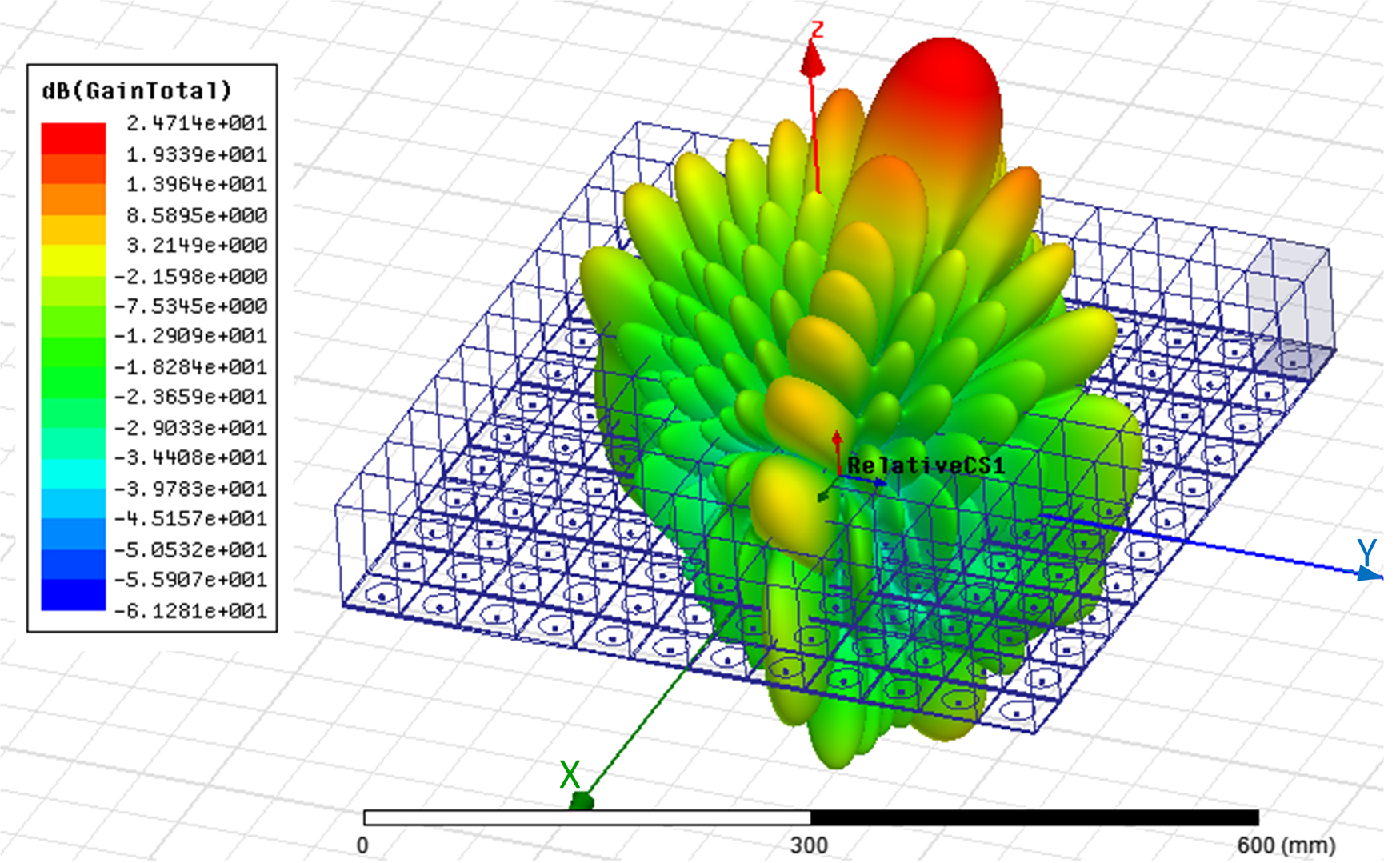
Fig. 17. Array model in HFSS and the radiation pattern of beam 1 with interleaved sub-arrays, P_x = P_y = 8, N_sx = N_sy = 4, N_x = N_y = 2, N_skx = N_sky = 4, d_x = d_y = 0.5λ, A_skrx = A_sklx = A_skry = A_skly = 0.7.

To illustrate the effects of interleaving sub-arrays in the grating lobe elimination, a planar array designed by tile sub-arraying technique has been simulated in HFSS. This array is similar to the array of Fig. 16 in the number of beams, number of array elements, and the angular distance between adjacent beams. The amplitude distribution of this array is unique. In Fig. 18, the simulation results of this array have been presented. As is seen, the grating lobes have been appeared in the visible region.

Fig. 18. HFSS simulation results of a 12 × 12 planar array with tile sub-arrays, P_x = P_y = 8, N_sx = N_sy = 3, N_x = N_y = 4, d_x = d_y = 0.5λ.

Designing the block diagrams of BFN for multiple sub-beam array

Optimization results in Table 2 (third column) show that the number of sub-array elements is not equal to the number of beams. Consequently, the standard BM cannot be used to design the BFN. To design the BFN, the relations presented in the section “Devising the BFN” must be used.

As presented in (11), the extra phase shifts that must be applied to the right skirt elements are different for various beams. In the following paragraph, the extra phase shifts of the designed antenna array in the section “Array optimization concerning sub-beam concept” will be calculated. Optimization results showed that P _x = 4N _x, and N _x is even. Therefore, the extra phase shifts which should be added to the right skirt elements in each row are calculated using (23):

(23)$$\Delta \varphi _{x\_right}( {c_x} ) = \left\{{\matrix{ {\pi N_x-\displaystyle{\pi \over 4} = -\displaystyle{\pi \over 4}; \;\quad \quad \alpha_{xi} = 1, \; \;5{\rm \;( }c_x = 1) } \hfill \cr {\pi N_x-\displaystyle{{3\pi } \over 4} = -\displaystyle{{3\pi } \over 4}; \;\quad \alpha_{xi} = 2, \; \;6{\rm \;( }c_x = 2) } \hfill \cr {\pi N_x-\displaystyle{{5\pi } \over 4} = -\displaystyle{{5\pi } \over 4}; \;\quad \alpha_{xi} = 3, \; \;7 \;( c_x = 3) } \hfill \cr {\pi N_x-\displaystyle{{7\pi } \over 4} = -\displaystyle{{7\pi } \over 4}; \;\quad \alpha_{xi} = 4, \; \;8 \;( c_x = 4) } \hfill \cr } } \right.$$

Since P _y = 4N _y and N _y = 2, $\Delta \varphi _{y_{right}}( c_y)$ can be calculated similarly.

As indicated in (23), for the first BG which consists of beams A and E, a phase shift of −π/4 must be added to the right skirt elements. For the second BG, a phase shift of −3π/4 must be added to the right skirt elements. Similar conditions hold for BG3 and BG4. The total number of BGs in the x direction using (11) is equal to M _x. The corresponding in the y direction is denoted by M _y = P _y/N _y. In this design, M _x and M _y are equal to 4.

Using (14)–(18), for P _x = 8 and N _x = 2, the excitation signals of the first and second elements of each sub-array, which are related to a right skirt element (in BFN1), have been obtained as follows:

(24)$$E_1 = 0.5[ {( V_1 + V_5) + ( V_2 + V_6) + ( V_3 + V_7) + ( V_4 + V_8) } ] $$

(25)$$E_2 = e^{-( i\pi /8) }( \! - \!\! V_1 + V_5) + e^{-( i3\pi /8) }( \! - \!\!V_2 + V_6) + e^{-( i5\pi /8) }( \! - \!\! V_3 + V_7) + e^{-( i7\pi /8) }( \! - \!\! V_4 + V_8) $$

Therefore, BFN1 consists of four 180° hybrids with sum-ports exciting the first element of the sub-arrays and the corresponding right skirt element. In addition, the difference-ports excite the second element of the sub-arrays. There are four BGs, which need four different $\Delta \varphi _{x\_right}$ for feeding the relevant right skirt element, as calculated in (23). In addition, two-way power dividers are used to provide the required signals for the right skirt elements, consistent with (9). BFN1 block for the designed array is illustrated in Fig. 19(a).

Fig. 19. Block diagram of (a) BFN1, (b) BFN2, and (c) BFN3.

Using (19)–(20), the excitation signals of the first and second elements of the sub-array, which are related to the left skirt element (in BFN2), have been calculated in (26) and (27). The block diagram of BFN2 for the designed array is plotted in Fig. 19(b).

(26)$$E_1 = ( V_1 + V_5) + ( V_2 + V_6) + ( V_3 + V_7) + ( V_4 + V_8) $$

(27)$$\eqalign{E_2 & = 0.5[ {e^{-( i\pi /8) }( \! - \!\! V_1 + V_5) + e^{-( i3\pi /8) }( \! - \! \! V_2 + V_6) }\cr& + e^{-( i5\pi /8) }( \! - \! \! V_3 + V_7) + e^{-( i7\pi /8) }( \! - \! \! V_4 + V_8) ] }$$

Since the calculated A _skrx(k) and A _sklx(k) in Table 2 are unique for all amounts of the k, all BFN1s have the same power division ratios. Using similar reasoning, all BFN2s which are designed for different sub-arrays are identical.

For feeding the core elements which are not connected to any skirt element, the feed network in Fig. 19(c) has been designed.

The operating frequency band of the optimized antenna as mentioned in the section “Array optimization concerning sub-beam concept” is C-band. The designed BFN can be practically implemented by planar microwave circuits. The BFN consists of 180° hybrids, phase shifters, crossovers, and power dividers, which are usually realized by microstrip technology. In addition, using microstrip technology, construction cost and size of the structure are lower compared to the other microwave structures similar to waveguides and substrate integrated waveguides. The array row- and column-feeds can be easily stacked and integrated to take the shape of a compact box for the antenna BFN.

The overall antenna system configuration is illustrated in Fig. 20. In the array aperture, the row elements which are fed by different types of BFNs are shown by different colors. Also, the column elements which are fed by different types of BFNs are indicated by different filling patterns.

Fig. 20. Configuration of the designed antenna system.

As can be inferred from Fig. 20, each row is excited by a sheet that consists of 18 SABFNs, eight power dividers and some phase shifters to provide the required phase for each SABFN. As indicated in Fig. 20, input ports of the rows’ BFN sheets are fed by the columns’ BFN sheets. In this way, the required phase shifts between the rows have been provided.

The optimized multiple sub-beam antenna using interleaved sub-arraying technique has been compared with some other synthesizing methods. The comparison criteria in Table 3 are aperture size, BFN complexity, and SLL. The requirements for multiple beam antenna in Table 2 have been used for comparison purposes. As inferred from Table 3, the size of the proposed array with multiple sub-beams is intensively lower compared to other studies. In addition, BFNs which have been designed by other approaches are more complex than the proposed BFN in this paper.

Table 3. Comparison between multiple beam array synthesis techniques