


1. Introduction
Among various fundamental turbulence related problems, the reactive scalar in constant density turbulence needs to be addressed because of its peculiarities. On the one hand, the reactive scalar problem has been extensively studied in turbulent combustion (Libby & Williams Reference Libby and Williams1976; Peters Reference Peters2000; Pope Reference Pope2000; Chakraborty & Cant Reference Chakraborty and Cant2004; Demosthenous et al. Reference Demosthenous, Borghesi, Mastorakos and Cant2016; Zhao, Wang & Chakraborty Reference Zhao, Wang and Chakraborty2018a,Reference Zhao, Wang and Chakrabortyb), where rapid heat release due to species reactions leads to a strong interaction between turbulence and flames, either premixed or non-premixed. Because of the large change of the fluid density, reactions have here strong feedback effects on the fluid dynamics. Thus, the species are considered as active. On the other hand, in constant density turbulent flows scalars are typically treated as non-reactive and passive, which has been the research focus in the turbulence community (Kraichnan Reference Kraichnan1968; Monin & Yaglom Reference Monin and Yaglom1975; Shraiman & Siggia Reference Shraiman and Siggia2000; Warhaft Reference Warhaft2000; Mitrovic & Papavassiliou Reference Mitrovic and Papavassiliou2004). However, constant density reactive turbulent flows are ubiquitous as well. From the viewpoint of fundamental aspects, this topic has a special importance as it can enrich the understanding of turbulence physics. In applications, a number of meaningful scenarios of relevance exist and are here briefly presented.
To control the harmful effects of reactive pollutants, the study of chemically reactive atmospheric systems has attracted considerable attention, e.g. the impact of climate change on the chemical composition of the atmosphere (Brasseur et al. Reference Brasseur, Schultz, Granier, Saunois, Diehl, Botzet, Roeckner and Walters2006), or the formation and evolution of aerosol particles (Wang et al. Reference Wang, Kong, Marten, He and Donahue2020). Since the change of temperature associated to these processes is small, the flow is typically incompressible. A better understanding of the reactive scalar interaction and the effects of turbulence will be helpful for pollution controls. Another important example of the present topic is the behaviour of marine species in a turbulent environment. Typically the driving forcing to generate turbulence is induced by the interactions between the oceanic and atmospheric flows at the interface (Pearson & Fox-Kemper Reference Pearson and Fox-Kemper2018). The large-scale ocean circulation will also impose atmospheric fluxes of momentum, heat and moisture. How to model the species transport process, either in the interior or at the interface of the ocean is particularly relevant for biogeochemical studies. In such turbulent conditions, species interaction, in the form of reactions, are important or even determinant to the species evolutions. For instance, the mixing process at the ocean and atmosphere interface drives the pelagic food because of the light available for photosynthesis at the surface. Species interaction can be modelled as chemical or biological reactions, e.g. between preys and predators or species and nutrition (Powell & Okubo Reference Powell and Okubo1994; Lopez et al. Reference Lopez, Neufeld, Hernandez-Garcia and Haynes2001; Hernandez-Garcia & Lopez Reference Hernandez-Garcia and Lopez2004; Gros̆elj, Jenko & Frey Reference Gros̆elj, Jenko and Frey2015). Although in some situations rather strong turbulence can be induced by the organisms (Dewar Reference Dewar2009; Kunze Reference Kunze2019), for simplicity, the species are considered here as passive. Moreover, in chemical engineering, mixing processes involving reactions in incompressible turbulence occur in many industrial applications (Hill Reference Hill1976; Sykes et al. Reference Sykes, Parker, Henn and Lewellen1994).
Chemical reactions introduce various complexities to the passive scalar problem, e.g. new characteristic time scales and the nonlinear source of the governing equation (Lamb & Shu Reference Lamb and Shu1978; Heeb & Brodkey Reference Heeb and Brodkey1990; Molemaker & de Arellano Reference Molemaker and de Arellano1998). Komori et al. (Reference Komori, Hunt, Kanzaki and Murakami1991) simulated two reactants of second-order irreversible reaction introduced in different parts of the bounding surface of the turbulent flow. They developed a model with the Damköhler number based on the integral time scale to estimate the segregation parameter, which characterizes the mixing of reactants. Corrsin (Reference Corrsin1961) studied the mixing of a scalar contaminant undergoing a first-order chemical reaction in isotropic turbulence and he deduced theoretically the power spectrum of the reactive scalar in different wavenumber ranges. Pao (Reference Pao1964) investigated the dilute turbulent concentration fields of a multicomponent mixture with first-order reaction in an isothermal environment, and proposed a unified spectral transfer concept for deducing the scalar spectrum at large wavenumbers. For higher-order reactions, nonlinearities from the chemical sources are also introduced into the problem. O'Brien (Reference O'Brien1966, Reference O'Brien1971) worked on decaying second-order, isothermal reactions in turbulence. The asymptotic decay rate of the scalar energy was found as  $t^{-11/2}$ for the moderate reaction, and
  $t^{-3/2}$ for the rapid reaction. Lin & O'Brien (Reference Lin and O'Brien1974) proposed a theoretical connection between the probability density functions (p.d.f.s) of the reactive species and those of the non-reacting species, which are in general of easier theoretical/experimental access. Similar analysis was also made in studying the scalar mixing layer problem (Bilger & Krishnamoorthy Reference Bilger and Krishnamoorthy1991). Meyers, O'Brien & Scott (Reference Meyers, O'Brien and Scott1978) further derived the general solution of the p.d.f. equation for reactive scalars under some limiting conditions. The covariance between reactants and the corresponding model terms are important topics of turbulent mixing analyses as well (Lamb & Shu Reference Lamb and Shu1978; Heeb & Brodkey Reference Heeb and Brodkey1990). For the dual non-premixed reactants case, it was surprisingly found (Toor Reference Toor1969) that the covariance is almost invariant for very slow and very rapid second-order reactions.
Wu et al. (Reference Wu, Calzavarini, Schmitt and Wang2020) analysed the reversible multicomponent reactions in isotropic turbulence in the near equilibrium condition with almost zero net reaction rates. It was observed that at the close-to-equilibrium state, the reactive scalar fluctuations have a Gaussian distribution. Overall, the net reaction rate is much smaller than the turbulent advection term. Therefore, the energy spectra are essentially uninfluenced by the chemical reaction. Even so, the chemical processes tend to reorganize the spatial distribution of the reactive scalars, a reduced reactant concentration fluctuation and an enhanced correlation intensity were observed, at odds with the effects induced by turbulent mixing that increases fluctuations and removes relative correlations. One main finding was that the correlations of the scalar quantities can be quantified based on a unique control parameter, the Damköhler number based on the scalar Taylor scale ( $Da_{\theta }$), defined as the ratio between the time scale of scalar diffusion across a distance of the size of the scalar Taylor microscale and the globally averaged chemical reaction time scale. The larger the value of
  $Da_{\theta }$, the more depleted the scalar fluctuations were as compared with the fluctuations of a non-reactive scalar field in the same conditions, and vice versa.
However, reactive turbulent flows can be also in strongly non-equilibrium chemical conditions, i.e. they may have important net reaction rates due to different forward and backward rates. To gain deeper insights on this aspect, it is interesting to explore the cases where the net reaction rate is more important than the advection term or even dominant. In the present work, a two stream-fed like flowing system is proposed to ensure locally strong chemical reactions by solving the governing equations of the total scalar fields instead of their fluctuating components. This new configuration for studying passive reactive scalars is presented and characterized in a statistical sense. As a second step, p.d.f.s of scalar fields and of their reaction rates are investigated. Then a theoretical model based on the a priori knowledge of the p.d.f. of the non-reactive scalar is proposed for predicting the mean and fluctuation of the reactive scalars. This model is in good agreement with the numerical results when the forward reaction is dominant. The correlation coefficient and spectrum of variance of the reactive scalars are also examined to explore the interactions across spatial scales between the turbulent mixing and the chemical kinetics in such a configuration.
The rest of this paper is organized as follows. In § 2 the definitions of the configuration and problem studied in this work are provided. Section 3 elaborates the details of the numerical methods. Then in § 4 the modelling analysis and numerical results are presented and discussed. Finally the conclusions of this paper are summarized in § 5.
2. The model system
The reactions considered here are of the form
where  $\textrm {R}_1$,
  $\textrm {R}_2$ and
  $\textrm {P}$ denote the three involved reactants (or reactive scalars). The process is reversible with the respective forward and backward reaction rate coefficients
  $\gamma _1$ and
  $\gamma _2$. The reactants are assumed to undergo diffusion and to be transported in a passive manner by an incompressible velocity flow field upon which they do not exert any effect. The evolution equations for the velocity field
  $\boldsymbol {u}(\boldsymbol {x},t)$ and for the scalar concentrations (
 $R_1(\boldsymbol {x},t)$,
  $R_2(\boldsymbol {x},t)$ and
  $P(\boldsymbol {x},t)$) read as
 \begin{gather} \partial_t \boldsymbol{u}+(\boldsymbol{u}\boldsymbol{\cdot}\boldsymbol{\nabla})\boldsymbol{u}=\nu\Delta \boldsymbol{u}-\boldsymbol{\nabla} p/\rho+\boldsymbol{f}, \end{gather}
 \begin{gather}\boldsymbol{\nabla} \boldsymbol{\cdot} \boldsymbol{u} = 0, \end{gather}
and
 \begin{gather} \partial_t R_1+(\boldsymbol{u}\boldsymbol{\cdot}\boldsymbol{\nabla})R_1=D\Delta R_1- \gamma_1 R_1R_2+\gamma_2 P+\dot{s}_{R_1}, \end{gather}
 \begin{gather}\partial_t R_2+(\boldsymbol{u}\boldsymbol{\cdot}\boldsymbol{\nabla})R_2=D\Delta R_2-\gamma_1 R_1R_2+\gamma_2 P+\dot{s}_{R_2}, \end{gather}
 \begin{gather}\partial_t P+(\boldsymbol{u}\boldsymbol{\cdot}\boldsymbol{\nabla})P=D\Delta P+\gamma_1 R_1R_2-\gamma_2 P+\dot{s}_P. \end{gather}
Here  $p$ is the hydrodynamic pressure,
  $\rho$ is the constant fluid density,
  $\nu$ is the kinematic viscosity and
  $D$ is the species diffusivity (assumed identical for all species). The source terms
  $\dot {s}_{R_1}$,
  $\dot {s}_{R_2}$ and
  $\dot {s}_P$ are prescribed later below.
In the following analyses, to gain primary insights of the turbulent transport physics, a non-reactive species  ${T}$ is also considered for comparison with the governing equation
 \begin{equation} \partial_t T+(\boldsymbol{u}\boldsymbol{\cdot}\boldsymbol{\nabla})T=D\Delta T+\dot{s}_T, \end{equation}
where the molecular diffusion  $D$ is the same as for the reactive scalars and the source term
  $\dot {s}_{T} = \dot {s}_{R_1}$.
In previous work by Wu et al. (Reference Wu, Calzavarini, Schmitt and Wang2020) it was shown that large-scale statistically homogeneous and isotropic reactive scalar sources/sinks are not able to sustain a strong deviation from the chemical equilibrium, which instead needs to be realized by imposing non-zero mean gradient profiles for the reactants. Thus, we propose here a new flow configuration, which is schematically illustrated in figure 1. In a cubic domain a large-scale forcing term  $\boldsymbol {f}$ is exerted into the momentum equation (2.2a) to sustain a statistically stationary homogeneous and isotropic velocity field with periodic boundary conditions along the three directions. Differently, the scalar fields are periodic only in the
  $x$ and
  $y$ directions. Along the
  $z$ direction, the following Dirichlet boundary conditions are implemented:
 \begin{equation} \begin{cases} R_1=R_0, R_2=0, P=0, T=R_0 & \text{when $z=0$},\\ R_1=0, R_2=R_0, P=0, T=0 & \text{when $z=H$}. \end{cases} \end{equation}
Here  $H$ is the length of the domain in the
  $z$ direction and
  $R_0$ is the constant boundary condition.

Figure 1. Schematic diagram of the flow configuration and computational domain. For the scalar quantities, the periodic boundary conditions are set along  $x$ and
  $y$ directions, while a Dirichlet boundary condition is used along the
  $z$ direction. The shadowed layers near the boundaries are the ‘buffer layers’ generated artificially, in which the quantities of scalars are close to the preset boundary values, as defined in (2.6). The part between buffer layers is denoted as the bulk region. Such a set-up is statistically stationary and ensures the local positiveness of scalar concentrations because it evolves directly the scalar concentration field rather than its fluctuation with respect to a mean background profile.
Numerically it is found that to realize reasonably large fluctuations for the scalar fields, buffer layers where the scalar are kept approximately constant in the vicinity of the Dirichlet boundaries are needed, as shown in figure 1 by the shadowed parts with the bulk region in between. Inside both the upper and bottom buffer layers, the artificial sources  $\dot {s}_{\theta }$ with
  $\theta =R_1,R_2,P$ or
  $T$ are added in the scalar equations, (2.3) and (2.4). Specifically,
  $\dot {s}_{\theta }$ is designed here as
 \begin{equation} \dot{s}_{\theta}= \begin{cases} \dfrac{1}{\tau}(\theta_0-\theta) & \text{in the buffer with $z\in[H-\delta,H]$ or $z\in[0,\delta]$} \\ 0, & \text{in the bulk with $z\in(\delta,H-\delta)$}. \end{cases} \end{equation}
Here  $\theta _0$ is the boundary value of
  $\theta$, as defined by the Dirichlet boundary conditions in (2.5);
  $\tau$ is a characteristic time scale to control the strength of the source terms. Small values of
  $\tau$ imply a fast source capable of efficiently maintaining the scalar values close to the boundary values. In our present simulation cases,
  $\tau$ is set on the order of the Kolmogorov time scale of the turbulent flow
  $\tau _\eta$, which is numerically
  $100$ times the simulation time step. Another parameter,
  $\delta$, is the buffer layer thickness, which can be tailored to adjust the scalar source (i.e. a larger thickness corresponds to a larger species source) and the scalar mean gradient.
3. Numerical implementation
First of all, it is convenient to non-dimensionalize the above set of equations by choosing reference scales appropriate for the present system. The domain size  $H$, the overall scalar difference
  $R_0$ in (2.5) and the overall fluctuating velocity
  $u'$ (single-component root-mean-square (r.m.s.) velocity obtained from the average over the three-dimensional domain and in time) are used as the reference quantities for the length scale, scalar and velocity, respectively. For simplicity, in the following, the quantities will be in dimensionless units without special notation. It then yields
 \begin{equation} \partial_t \boldsymbol{u}+(\boldsymbol{u}\boldsymbol{\cdot}\boldsymbol{\nabla}) \boldsymbol{u}=Re^{{-}1}\Delta\boldsymbol{u}-\boldsymbol{\nabla} p+\boldsymbol{f},\quad \boldsymbol{\nabla} \boldsymbol{\cdot} \boldsymbol{u} = 0, \end{equation}
 \begin{gather} \partial_t R_1+(\boldsymbol{u}\boldsymbol{\cdot}\boldsymbol{\nabla})R_1=(Sc\,Re)^{{-}1}\Delta R_1-Da_1R_1R_2+Da_2P+\dot{s}_{R_1}, \end{gather}
 \begin{gather}\partial_t R_2+(\boldsymbol{u}\boldsymbol{\cdot}\boldsymbol{\nabla})R_2=(Sc\,Re)^{{-}1}\Delta R_2-Da_1R_1R_2+Da_2P+\dot{s}_{R_2}, \end{gather}
 \begin{gather}\partial_t P+(\boldsymbol{u}\boldsymbol{\cdot}\boldsymbol{\nabla})P=(Sc\,Re)^{{-}1}\Delta P+Da_1R_1R_2-Da_2P+\dot{s}_P, \end{gather}
 \begin{gather}\partial_t T+(\boldsymbol{u}\boldsymbol{\cdot}\boldsymbol{\nabla})T=(Sc\,Re)^{{-}1}\Delta T+\dot{s}_T, \end{gather}
where  $Re=H u'/\nu$ is the Reynolds number; the Schmidt number
  $Sc=\nu /D$ is the ratio of viscous diffusion to molecular diffusion; the ratios of the flow time scale to the chemical time scales of forward and backward reaction define the Damköhler numbers
  $Da_1=H \gamma _1 R_0/u'$ and
  $Da_2= H \gamma _2/u'$, respectively, and
  $\varGamma =Da_1/Da_2$ characterizing the relative importance of the forward reaction to the backward reaction. The dimensionless boundary conditions (for scalars) are
 \begin{equation} \begin{cases} R_1=1, R_2=0, P=0, T=1 & \text{when $z=0$},\\ R_1=0, R_2=1, P=0, T=0 & \text{when $z=1$}. \end{cases} \end{equation}
 In this study,  $Da_2$ is set as constant and
  $Da_1$ is varied. The key involved parameters in the present simulations are listed in table 1. For the near equilibrium case in the previous work by Wu et al. (Reference Wu, Calzavarini, Schmitt and Wang2020), the forward and backward reactions almost balance each other and, thus, only one Damköhler number was needed to describe the reaction intensity of the reaction. However, for the present configuration at strongly non-equilibrium state, the global forward and backward reactions are apparently different. As shown in figure 2 with the increase of
  $\varGamma$, the global forward rate, estimated by
  $Da_1\langle R_1 R_2\rangle$, is clearly larger than the global backward rate
  $Da_2\langle P\rangle$, where
  $\langle \cdot \rangle$ means the average in time and the
  $x$–
$x$– $y$ plane at a specific
  $z$.
$z$.
Table 1. Non-dimensionalized parameters for the simulations:  $Re= u'H/\nu$ is the Reynolds number based on large scale, where
  $u'$ is the single-component r.m.s. velocity,
  $H$ is the size of the simulation domain,
  $\nu$ is the viscosity;
  $Re_{\lambda } = u'\lambda /\nu$ is the Taylor scale
  $\lambda$-based Reynolds number;
  $Sc$ is the Schmidt number (
 $\nu /D$);
  $N^3$ is the number of total grid points;
  $|\boldsymbol {k}|_{max}\cdot \eta$ is the resolution condition, where
  $|\boldsymbol {k}|_{max}$ is the maximum amplitude of the wavenumber kept by the dealiasing procedure,
  $\eta$ if the Kolmogorov length scale;
  $\tau _\eta$ is the Kolmogorov time scale;
  $\varGamma =Da_1/Da_2$, with
  $Da_1$ and
  $Da_2$ as the Damkholer numbers for forward and backward reactions, respectively;
  $L_I$ is the integral length scale;
  $T_I$ is the integral time scale;
  $\Delta t$ is the numerical time step.

Figure 2. The reaction rates computed from the mean quantities as functions of  $z$. The solid lines are for the forward reaction rates
  $Da_1\langle R_1R_2\rangle$ and the dashed lines are for the backward reaction rates
  $Da_2\langle P\rangle$. A clear difference can be observed. Vertical dotted lines mark the interfaces between the buffer layers and the bulk region.
The statistically stationary homogeneous and isotropic turbulent flow is sustained by a large-scale forcing term (Eswaran & Pope Reference Eswaran and Pope1988; Mansour & Wray Reference Mansour and Wray1994; Sripakagorn et al. Reference Sripakagorn, Mitarai, Kosály and Pitsch2004; Hou & Li Reference Hou and Li2007), whose expression in the Fourier space  $\hat {\boldsymbol {f}}(\boldsymbol {k},t)$ reads as
 \begin{equation} \hat{\boldsymbol{f}}(\boldsymbol{k},t)=\frac{1}{\tau_f}\sum_{1\leqslant|\boldsymbol{k}|\leqslant2\sqrt{2}}\hat{\boldsymbol{u}}(\boldsymbol{k},t). \end{equation}
Here  $\tau _f$ is a time scale to be adjusted at each time step in order to provide a constant power input, i.e.
  $\int _V \boldsymbol {f}\boldsymbol {\cdot }\boldsymbol {u}\, {{\rm d} x}^3= {\rm const}.$ (Schumacher, Sreenivasan & Yakhot Reference Schumacher, Sreenivasan and Yakhot2007). Note that the zeroth mode
  $|\boldsymbol {k}|=0$ is not forced in order to prevent the development of a global mean flow, i.e.
  $\int _V \boldsymbol {u}\, {{\rm d} x}^3= \boldsymbol{0}$. The isotropic velocity field is obtained by numerically solving (3.1a,b) using a pseudo-spectral code (Gauding, Danaila & Varea Reference Gauding, Danaila and Varea2017, Reference Gauding, Danaila and Varea2018) with a smooth dealiasing technique (Hou & Li Reference Hou and Li2007) for the treatment of nonlinear terms in the equations. Differently, the scalar equations (3.2) are solved by the finite difference method with an eighth-order upwind scheme (using five upstream grids and three downstream grids) and a tenth-order centre scheme for the first- and second-order spatial derivatives, respectively.
The velocity field is initialized by prescribing the spectrum of kinetic energy in the Fourier space  $\hat {\boldsymbol {u}}(\boldsymbol {k};0)$ (Schumacher et al. Reference Schumacher, Sreenivasan and Yakhot2007), where both the modulus and phases are randomly determined, under the constraint of zero mean (
 $\hat {\boldsymbol {u}}(\boldsymbol {0};0)=\boldsymbol{0}$) and prescribed kinetic energy spectrum of
 \begin{equation} E(k;0)=\sum_{k=|\boldsymbol{k}|}\left|\hat{\boldsymbol{u}}(\boldsymbol{k};0)\right|^2\propto |\boldsymbol{k}|^4\,{\rm e}^{{-}2(|\boldsymbol{k}|/2)^2}. \end{equation}
The scalars are linearly initialized as
 \begin{equation} \begin{cases} R_1(x,y,z;0) = 1-z,\\ R_2(x,y,z;0) = z,\\ P(x,y,z;0) = 0,\\ T(x,y,z;0) = 1-z. \end{cases} \end{equation}
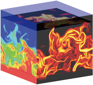
 Figure 3 shows a visualization of the  $R_1$ field and of the reaction rate (
 $Da_1R_1R_2-Da_2P$) on the isosurface of
  $R_1=0.5$ under the condition of
  $\varGamma =10$. It can be seen that with the properly defined buffer layer, the spatial fluctuation of scalar can be self-sustained with the total scalar quantities perfectly confined in the prescribed
  $[0,1]$ range.

Figure 3. The three-dimensional instantaneous snapshots of (a)  $R_1$, and (b) reaction rate (
 $Da_1R_1R_2-Da_2P$) on the isosurface of
  $R_1=0.5$, under the condition of
  $\varGamma =10$.
The statistical stationarity of the set-up can be appreciated from the temporal evolution of the scalar statistical moments. As an example, figure 4 shows that the evolutions of the spatial averages of scalar concentrations and r.m.s.s of scalar fluctuations in the bulk region with  $z\in [\delta,1-\delta ]$ for the case
  $\varGamma = 10$. This indicates that the reacting system is strongly deviated from chemical equilibrium. The following analyses will be focused on the bulk region. Data samples are collected in a time span of about ten times the integral time
  $T_I=k/\epsilon$ with
  $k = 3u'^2/2$, once the statistically stationary state is reached.

Figure 4. Evolution of the spatial averages of scalar concentrations and r.m.s. of scalar fluctuations in the bulk region with  $z\in [\delta, 1-\delta ]$ for the case of
  $\varGamma = 10$. Time is normalized by the integral time
  $k/\epsilon$ with
  $k = 3u'^2/2$. The dashed vertical lines mark the initial time for the computation of statistical quantities.
4. Result analyses
4.1. Properties of the buffer layer and the bulk region
In the present configuration the two buffer layers function as a source which sustains the mean scalar gradient, while the bulk domain is where the turbulent mixing occurs and where the present analysis is focused. The means and r.m.s. of the fluctuations of the non-reactive scalars ( $T$) in the configurations with different buffer layer thickness
  $\delta$ are shown in figures 5(a) and 5(b), respectively. As can be expected, in the bulk region the mean scalar profile follows a linear relation with respect to
  $z$, i.e. constant gradient, under the action of isotropic turbulent velocity. From the prescribed geometrical and boundary conditions, the constant gradient is about
  $1/(1-2\delta )$.

Figure 5. Numerical profiles of (a) the mean, and (b) the r.m.s. of  $T$ with different buffer layer thickness
  $\delta$. The vertical dotted lines mark the interfaces between the buffer layers and the bulk region.
For the scalar fluctuation, figure 5(b) demonstrates that in the bulk region the scalar r.m.s. is almost constant, similar to the homogeneous shear turbulence (Mellado, Wang & Peters Reference Mellado, Wang and Peters2009). In most of the buffer layer, the scalar r.m.s. is negligibly small, because the strong modulation effect from the source term  $\dot {s}_T$ makes the scalar
  $T$ roughly constant. Specifically, the strength of such a modulation is determined by the control parameter
  $\tau$. In this sense, the present flow can be effectively tailored by the control parameters
  $\tau$ and
  $\delta$.
Further insights of the relation between the buffer and bulk regions can be gained by the following analytical approach. First, the mixing length hypothesis is adopted to model the Reynolds stress as
 \begin{equation} \langle {u}_z T\rangle={-}D_T\frac{\partial \langle T\rangle}{\partial z}, \end{equation}
where  $D_T$ is the turbulent diffusivity and considered as constant (a hypothesis which will be numerically validated later). The ensemble average (
 $\langle \cdot \rangle$) of (3.2d) then yields
 \begin{equation} \partial_t \langle T\rangle=(D_T+D)\varDelta \langle T\rangle+\langle\dot{s}_T\rangle. \end{equation}
Because of symmetry, only half of the domain in the range of  $z\in [0,1/2]$ needs to be studied. Under the statistical stationary condition, the temporal derivative term in (4.2) vanishes. Let us denote
  $D_T$ in the bulk region and buffer layer as
  $D_{T,1}$ and
  $D_{T,2}$, respectively. Combining the specific form of
  $\dot {s}_T$ (2.6) and neglecting the laminar diffusivity
  $D$ in (4.2), an ordinary differential equation about
  $\langle T\rangle$ is then found, i.e.
 \begin{equation} \begin{cases} D_{T,2}\dfrac{{\rm d}^2 \langle T\rangle}{{\rm d}z^2}=\dfrac{1}{\tau}(\langle T\rangle-1) & \text{ when $0\leqslant z\leqslant\delta$} ,\\ D_{T,1}\dfrac{{\rm d}^2 \langle T\rangle}{{\rm d}z^2}=0 & \text{ when $\delta\leqslant z\leqslant 1/2$} . \end{cases} \end{equation}
 The numerical value of  $D_T$, calculated according to (4.1), is shown in figure 6(a). From the analytical point of view, we approximate
  $D_{T,1}$ and
  $D_{T,2}$ as
  $z$-independent constants. Similar to the r.m.s. profile of
  $T$,
$T$,  $D_T$ is also negligibly small in most of the buffer layer, following the same modulation mechanism as for the source
  $\dot {s}_T$. Specifically, the controlling parameter
  $\tau$ leads to a small value of
  $D_{T,2}$, while physically
  $D_{T,1}$ is determined by the flow integral time
  $T_I$. Thus, we further assume that
  ${D_{T,2}}/{D_{T,1}}=K({\tau }/{T_I})$, where the proportionality coefficient
  $K$ (
$K$ ( $K=O(1)$) needs to be determined numerically. As stated in the last paragraph,
  $K=4$ can give us a good fitting result.

Figure 6. (a) Turbulent diffusivity calculated from (4.1). (b) Theoretical prediction of the mean of  $T$ (dashed lines) compared with the DNS results (solid lines with the same colour). The vertical dotted lines mark the interfaces between the buffer layers and the bulk region.
To solve this set of ordinary differential equations, four boundary conditions are needed, including  $\langle T\rangle (0)=1$,
  $\langle T\rangle (1/2)=1/2$, the continuity of
  $\langle T\rangle$ at
  $z=\delta$ and the continuity of the flux of
  $\langle T\rangle$ at
  $z=\delta$. Because of the different diffusivity in the buffer layer and the bulk region, the continuity of the flux of
  $\langle T\rangle$ at
  $z=\delta$ can be expressed as
 \begin{equation} D_{T,2}\frac{{\rm d}\langle T\rangle}{{\rm d}z}(z\rightarrow\delta^-)=D_{T,1}\frac{{\rm d}\langle T\rangle}{{\rm d}z}(z\rightarrow\delta^+). \end{equation}
Therefore, the analytical solution of (4.3) for  $\langle T\rangle$ is obtained as
 \begin{equation} \langle T\rangle(z)= \begin{cases} C_1\sinh\left(\sqrt{\dfrac{1}{D_{T,2}\tau}}z\right)+1 & \text{ when $0\leqslant z\leqslant\delta$} ,\\ C_2 z+C_3 & \text{ when $\delta\leqslant z\leqslant 1/2$}. \end{cases} \end{equation}
The analytical expression for the constant coefficients  $C_1, C_2, C_3$ can be found in Appendix A. Numerically, it is found that the model solution with
  ${D_{T,2}}/{D_{T,1}}= 4({\tau }/{T_I})$ matches direct numerical simulation (DNS) results well, as shown in figure 6(b). In summary, the difference between the buffer layer and the bulk region is mainly induced by the different turbulent diffusivity, because of the strong modulation effect from the source term
  $\dot {s}_T$ (and other
  $\dot {s}$ terms as well) in the buffer. In the following analyses, the buffer layer thickness
  $\delta$ is set constant
  $1/8$, as listed in table 1.
4.2. Probability density functions
In this section we focus on the difference between the  $z$-dependent statistical properties of the reactive and non-reactive scalars, or the effects of the chemical reaction. It can be seen from (3.2) and the corresponding boundary conditions (3.3) that
  $R_1(z)= R_2(1-z)$ statistically, i.e.
  $R_1$ and
  $R_2$ are symmetric with respect to the middle of the domain with
  $z=1/2$. Therefore, for the sake of brevity, the results for
  $R_2$ will be omitted in the remaining analyses.
Figure 7 shows on the middle plane with  $z=1/2$ the p.d.f.s of the scalar quantities
  $R_1$ and
  $P$, together with that of the non-reactive scalar
  $T$. Overall, the p.d.f. of
  $T$, denoted as
  $p_T$, is symmetric and has a central maximum at
  $T=0.5$. Moreover, since the effect of the buffer layers can be compared with the mixing process in the shear layer, two other local peaks appear at the tails of
  $p_T$ at
  $T=0$ and
  $T=1$ (same for the other p.d.f.s) (Mellado et al. Reference Mellado, Wang and Peters2009). Larger
  $\varGamma$ lead to a stronger skew of
  $p_{R_1}$ toward the
  $R_{1}=0$ side. Such a skewness property is the consequence of chemical reactions, because faster forward chemical reactions tend to deplete the reactants
  $R_1$ and
  $R_2$ but enrich the product
  $P$, enhancing
  $p_{R_1}$ at the
  $R_{1}=0$ end and extending the
  $p_P$ toward the larger
  $P$ side.

Figure 7. Dependence of p.d.f.s at  $z=1/2$ on
  $\varGamma$ for (a)
  $R_1$ and
  $T$, and (b)
  $P$. The insert panel in (b) plots the peak of
  $p_P$ as a function of
  $\varGamma$.
At different  $z$ values the scalar concentration p.d.f.s are shown in figure 8(a) for
  $R_1$ and figure 8(b) for
  $T$. We can see clearly the mirror symmetry between
  $p_T(z)$ and
  $p_T(1-z)$, which, however, breaks down for the
  $R_1$ case, because of the strong influence from the chemical sources. In addition, the p.d.f. of
  $T$ is of particular importance. In the modelling analysis discussed in the following section, the moments of the reactive scalars can be theoretically predicted based on
  $p_T$ undergoing the same turbulent environment.

Figure 8. Probability density functions of (a)  $R_1$ under the condition of
  $\varGamma =10$ and (b)
  $T$ at different positions.
The dependence of the p.d.f. of the net reaction rate  $R_{net}=Da_1R_1R_2-Da_2P=Da_1(R_1R_2-P/\varGamma )$ on
  $\varGamma$ is presented in figure 9 (at
  $z=1/2$). Toward the fast chemical limit with large
  $\varGamma$, the p.d.f. peaks higher at the
  $R_{net}=0$ end and meanwhile becomes more extended toward the higher
  $R_{net}$ side. When
  $Da_1$ and
  $Da_2$ are comparable, the p.d.f. peaks at some moderate value of
  $R_{net}$. Since all the cases are under the control of the identical turbulence velocity, such a difference must be caused by the chemical mechanism, which can be more clearly viewed from the spatial distribution of the reaction rates. From the comparison between figures 10(a) and 10(d), there is a clear difference between the distribution of
  $R_{net}$ for
  $\varGamma =100$ and
  $\varGamma =1$. For large
  $\varGamma$ (and large
  $Da_1$ as well), the large
  $R_{net}$ regions are highly concentrated in thin stripes, while for small
  $\varGamma$, regions with high
  $R_{net}$ are much more broadly distributed, which explains the local bump in the p.d.f. profile in figure 9. A more detailed understanding of such a property can be clarified from the separated results of the forward and backward reaction rates. It can be seen that a similar difference appears between figures 10(b) and 10(e), while, figures 10(c) and 10(f) are weakly influenced or even uninfluenced by
  $\varGamma$. Because the forward reaction rate is determined by the correlation between
  $R_1$ and
  $R_2$, larger
  $\varGamma$ will enhance the correlation (Wu et al. Reference Wu, Calzavarini, Schmitt and Wang2020) and meanwhile reduce in most of the flow field their coexistence, which explains the stripe-like distribution in figure 10(a). Since for the present chemical kinetics the backward reaction rate is solely determined by
  $P$, the effect of
  $\varGamma$ on the correlation between
  $R_1$ and
  $R_2$ is not relevant in determining the backward reaction rate. Therefore, figures 10(c) and 10(f) are almost identical. In summary, under different
  $\varGamma$ the p.d.f. and spatial distribution of the net reaction rate will be mainly determined by the forward part.

Figure 9. Probability density functions of the reaction rate ( $Da_1R_1R_2-Da_2P$) under the conditions of different
  $\varGamma$, at the position of
  $z=1/2$.

Figure 10. The instantaneous two-dimensional snapshot of reaction rate at the position of  $z=1/2$. The upper row (a–c) corresponds to
  $\varGamma =100$; the lower row (d–f) corresponds to
  $\varGamma =1$. The first column (a,d) shows the net reaction rate (
 $Da_1R_1R_2-Da_2P$); the second column (b,e) shows the forward reaction rate (
 $Da_1R_1R_2$); the third column (c,f) shows the backward reaction rate (
 $Da_2P$).
4.3. Moments of the reactive scalars
The reactive scalar  $\theta$ (e.g.
  $R_1$,
  $R_2$ or
  $P$) can be decomposed into the
  $z$-dependent mean part and the fluctuating part as
  $\theta (\boldsymbol {x},t) = \langle \theta \rangle (z,t) + \theta '(\boldsymbol {x},t)$, whose numerical results are shown in figure 11.

Figure 11. The mean (solid lines) and r.m.s. (dashed lines) of (a)  $R_1$ compared with
  $T$; (b)
  $P$ under the conditions of different
  $\varGamma$ as functions of position (
 $z$). The main panel of (c) shows the mean profile of
  $P$ normalized by its maximum, whose function as
  $\varGamma$ is plotted in the inset plot. There is a perfect superposition for all
  $\varGamma$ values. In all the plots, the vertical dotted lines mark the interfaces between the buffer layers and the bulk region.
Different from the linear profile of the non-reactive scalar  $T$, the profiles of
  $\langle R_1 \rangle$ are concave in the bulk region, because of chemical consumption of
  $R_1$ with
  $R_2$. With increasing
  $\varGamma$,
  $\langle R_1\rangle$ decreases while
  $\langle P\rangle$ increases, because a stronger forward reaction depletes more
  $R_1$ and produces more
  $P$. The scalar means tend to saturate at infinite large
  $\varGamma$. Interestingly, figure 11(c) shows that the normalized
  $\langle P\rangle$ by the corresponding maximum overlaps for different
  $\varGamma$, which suggests a kind of universality of
  $\langle P\rangle$.
Concerning the fluctuation of  $R_1$, in the upper half of the domain, i.e.
  $z>1/2$, larger
  $\varGamma$ leads to a smaller fluctuation, while in the lower half with
  $z<1/2$, larger
  $\varGamma$ leads to a larger fluctuation. From the gradient hypothesis, in isotropic turbulence the r.m.s. of
  $R_1$ is reasonably determined by its mean gradient, i.e. the larger means gradient leads to a larger fluctuation, as shown in figure 11(a). Close to the middle plane where
  $z$ is slightly greater than
  $1/2$, the gradient of
  $\langle R_1 \rangle$ is equal to that of
  $\langle T \rangle$, resulting in equality of the r.m.s. of
  $R_1$ and the r.m.s. of
  $T$. For the product
  $P$, its r.m.s. reaches a maximum at the edge of the bulk region and a minimum in the middle (
 $z=1/2$). Physically, the fluctuation of
  $P$ is jointly determined by the chemical kinetics, the fluctuations of
  $R_1$ and
  $R_2$, and the turbulent mixing. At the edge of the bulk, the r.m.s. of
  $R_1$ is large, but
  $R_2$ fluctuates weakly, which can not lead to a high peak of the r.m.s. of
  $P$. Therefore, such a maximum must be dominated by the turbulent mixing, or specifically, by the large gradient of
  $\langle P\rangle$ close to the bulk edge (see the
  $\langle P\rangle$ results) due to the gradient hypothesis. In parallel, at
  $z=1/2$ the gradient of
  $\langle P\rangle$ and the turbulent transport part vanish, leading to the minimum of the r.m.s. of
  $P$ at
  $z=1/2$.
It is also fundamentally interesting to investigate the scaling relation of the means and fluctuations with  $\varGamma$. As presented in figure 12, statistical results at different
  $z$ do not show any scaling behaviour. To have further understanding of the effects of the chemical reaction on the scalar moments, the present reactive turbulent system needs to be investigated theoretically. The following analyses will be based on the results of the non-reactive species
  $T$, instead of directly from the governing equations of scalar moments, because of the intractably complex higher-order terms involved.

Figure 12. Dependence of (a) the scalar means and (b) the scalar fluctuations on  $\varGamma$. There is no scaling behaviour in different flow regions.
Let us define  $X=R_1-R_2$. Subtracting (3.2a) from (3.2b) yields
 \begin{equation} \partial_t X+(\boldsymbol{u}\boldsymbol{\cdot}\boldsymbol{\nabla})X=(Sc\,Re)^{{-}1}\Delta X+\dot{s}_{R_1}-\dot{s}_{R_2}, \end{equation}
with boundary conditions of
 \begin{equation} \begin{cases} X=1 & \text{when $z=0$},\\ X={-}1 & \text{when $z=1$}. \end{cases} \end{equation}
Comparing the governing equation and boundary conditions of  $X$ with that of the non-reactive scalar
  $T$ (3.2d) and (3.3) yields
 \begin{equation} X=R_1-R_2=2T-1. \end{equation}
Let us define  $p_X(x;z)$ as the p.d.f. of
  $X$ at the position of
  $z$ (similar definition for other random quantities). Relation (4.8) gives
 \begin{equation} p_X(x;z)=\frac{1}{2}p_T\left(\frac{x+1}{2};z\right). \end{equation}
 First consider the case of infinitely large  $Da_1$. This implies that
  $R_1$ and
  $R_2$ cannot coexist because of the infinite chemical source
  $Da_1R_1(\boldsymbol {x},t)R_2(\boldsymbol {x},t)$, leading to
  $R_1(\boldsymbol {x},t)R_2(\boldsymbol {x},t)\!=\!0$. Therefore, a positive
  $X(\boldsymbol {x},t)$ is equivalent to
  $R_1(\boldsymbol {x},t)=X(\boldsymbol {x},t)$ and
  $R_2(\boldsymbol {x},t)=0$, while
  $X(\boldsymbol {x},t)<0$ implies that
  $R_1(\boldsymbol {x},t)=0$ and
  $R_2(\boldsymbol {x},t)=-X(\boldsymbol {x},t)$. For the quantity
  $P$, subtracting (3.2d) from (3.2a), together with the boundary conditions, we conclude that
 \begin{equation} P(\boldsymbol{x},t)=T(\boldsymbol{x},t)-R_1(\boldsymbol{x},t). \end{equation}
Therefore, a relation between  $P(\boldsymbol {x},t)$ and
  $X(\boldsymbol {x},t)$ can be obtained directly. Here, the infinitely large
  $Da_1$ leads to the following relations:
 \begin{equation} \begin{cases} R_1(\boldsymbol{x},t)=2T(\boldsymbol{x},t)-1, R_2(\boldsymbol{x},t)=0, P(\boldsymbol{x},t)=1-T(\boldsymbol{x},t) & \text{when } T(\boldsymbol{x},t)\geqslant1/2;\\ R_1(\boldsymbol{x},t)=0, R_2(\boldsymbol{x},t)=1-2T(\boldsymbol{x},t),P(\boldsymbol{x},t)=T(\boldsymbol{x},t) & \text{when } T(\boldsymbol{x},t)<1/2. \end{cases} \end{equation}
 Consequently, given that the non-reactive scalar field  $T$ is known, the mean and r.m.s. of
  $R_1$ (at infinite
  $\varGamma$) can be respectively determined as
 \begin{align} \langle R_1\rangle(z)&=\int_{0}^1 x p_X(x;z)\,{{\rm d} x}= \int_{0}^1 \frac{1}{2}x p_T\left(\frac{x+1}{2};z\right){{\rm d} x}\nonumber\\ &=2\left\langle T|T>\frac{1}{2}\right\rangle(z)-\int_{{1}/{2}}^1p_T(t;z)\,{\rm d}t, \end{align}
and
 \begin{align} \langle R_1'^2\rangle(z)&=\langle R_1^2\rangle(z)-\langle R_1\rangle^2(z)\nonumber\\ &=\int_{0}^1 \frac{1}{2}x^2 p_T\left(\frac{x+1}{2};z\right){{\rm d} x}- \left[\int_{0}^1 \frac{1}{2}x p_T\left(\frac{x+1}{2};z\right)\,{{\rm d} x}\right]^2. \end{align}
A similar derivation can be done for  $P$. The predictions are shown in figure 13 and 14. We note that an interesting analogy for a reactive flow at the diffusion limit leading to an expression for the p.d.f.s of reactive species obtained in terms of the p.d.f.s of non-reactive ones was proposed by Lin & O'Brien (Reference Lin and O'Brien1974).

Figure 13. The scalar mean (a)  $\langle R_1\rangle$ and (b)
  $\langle P\rangle$ as functions of
  $z$ obtained from theoretical analysis (dashed lines) based on (4.15) and DNS (solid lines with the same colours). The grey dashed lines are from the theoretical prediction at infinitely large
  $Da_1$ according to (4.12). We see that the prediction for
  $\varGamma =\infty$ is close to the curves for
  $\varGamma =100$ and also the predictions for large
  $\varGamma$ are close to the DNS results when
  $\varGamma =10$, 30, 100. The vertical dotted lines mark the interfaces between the buffer layers and the bulk region.

Figure 14. The scalar fluctuations (a)  $\langle R_1'^2\rangle ^{1/2}$ and (b)
  $\langle P'^2\rangle ^{1/2}$ as functions of
  $z$ obtained from theoretical analysis (dashed lines) and DNS (solid lines with the same colours). The grey dashed lines are from the theoretical prediction at infinitely large
  $Da_1$ according to (4.13). We see that the prediction for
  $\varGamma =\infty$ is close to the curves for
  $\varGamma =100$ and also the predictions for large
  $\varGamma$ are close to the DNS results when
  $\varGamma =10$, 30,
  $100$. The vertical dotted lines mark the interfaces between the buffer layers and the bulk region.
For the finite but large  $\varGamma$,
  $R_1(\boldsymbol {x},t)$ and
  $R_2(\boldsymbol {x},t)$ can locally coexist, i.e.
  $R_1R_2>0$. Since the overall forward reaction is still strong (if
  $\varGamma$ is sufficiently larger than unity), we assume here that there exits an upper limit for
  $R_1(\boldsymbol {x},t)R_2(\boldsymbol {x},t)$, i.e.
 \begin{equation} R_1(\boldsymbol{x},t)R_2(\boldsymbol{x},t)\leqslant\frac{C}{\varGamma}, \end{equation}
where  $C$ is a constant to be determined. Moreover, for any given
  $X(\boldsymbol {x},t)\in [-1,1]$, another constraint is
  $R_1(\boldsymbol {x},t)R_2(\boldsymbol {x},t)\leqslant 1-|X(\boldsymbol {x},t)|$ (Appendix B). Putting these together, it gives
  $R_1R_2\in [0, \min ({C}/{\varGamma },1-|X(\boldsymbol {x},t)|)]=[0,\beta _{max}]$. For a given
  $X(\boldsymbol {x},t)=\alpha$ and
  $R_1(\boldsymbol {x},t)R_2(\boldsymbol {x},t)=\beta$,
  $R_1=({\alpha +\sqrt {\alpha ^2+4\beta }})/{2}$. If the conditional p.d.f. of
  $R_1R_2$ on
  $X$, i.e.
  $p_{R_1R_2|X}(\beta |\alpha ;z)$, is known,
  $\langle R_1\rangle$ as a function of
  $z$ can be determined as
 \begin{equation} \langle R_1\rangle(z)=\int_{{-}1}^1 p_X(\alpha;z) \int_{0}^{\beta_{max}} \frac{\alpha+\sqrt{\alpha^2+4\beta}}{2} p_{R_1R_2|X}(\beta|\alpha;z)\,{\rm d}\beta \,{\rm d}\alpha . \end{equation}
A hypothesis assumed here is that with given  $X(\boldsymbol {x},t)$,
  $R_1(\boldsymbol {x},t)R_2(\boldsymbol {x},t)$ is uniformly distributed in
  $[0,\beta _{max}(\alpha )]$. Together with the numerical results of the p.d.f. of the non-reactive scalar
  $T$, the mean
  $\langle R_1\rangle (z)$ and variance
  $\langle R_1'^2\rangle (z)=\langle R_1^2\rangle (z)-\langle R_1\rangle ^2(z)$ can then be calculated (similar analyses for
  $R_2$ and
  $P$). As shown in figures 13 and 14, when
  $\varGamma \geqslant 10$, the modelling and numerical results can satisfactorily match if the constant
  $C$ in (4.14) is set as
  $0.7$. When
  $\varGamma <10$, these predictions do not hold.
4.4. Correlation coefficients
For scalars  $\theta _1$ and
  $\theta _2$ under consideration, the correlation coefficients are defined (based on the fluctuating parts) as
 \begin{equation} r(\theta_1,\theta_2)(z) = \frac{\langle \theta_1'\theta_2'\rangle}{\langle \theta_1'^2\rangle^{1/2}\langle \theta_2'^2\rangle^{1/2}}. \end{equation}
 The scalar correlations are jointly determined by the chemical reaction and the turbulent mixing. Wu et al. (Reference Wu, Calzavarini, Schmitt and Wang2020) found that a competition exists between the chemical reaction and turbulent mixing. Specifically, the chemical reaction tends to dampen reactant concentration fluctuations and enhance their correlation intensity, while turbulent mixing increases fluctuations and removes relative correlations. Analytical results for the correlation coefficients have also been obtained thanks to the linear decomposition of each scalar concentration in terms of a large mean term and a small local fluctuation. In the present flow configuration the large local deviation from the chemical equilibrium invalidates the same linear decomposition approach. Numerical results of the  $z$-dependent correlation coefficients are shown in figure 15.

Figure 15. Direct numerical simulations of the correlation coefficients between (a)  $R_1$ and
  $R_2$; (b)
  $R_1$ and
  $P$ as functions of
  $z$, for different
  $\varGamma$ cases. The vertical dotted lines mark the interfaces between the buffer layers and the bulk region.
In figure 15(a),  $r(R_1,R_2)$ can be understood as follows. For the present non-equilibrium configuration, considering the limiting non-reactive case with
  $Da_{1,2}=0$, the sum of
  $R_1$ and
  $R_2$ becomes constant and, consequently,
  $r(R_1,R_2)=-1$, i.e.
  $R_1$ and
  $R_2$ are perfectly negatively correlated. At non-zero
  $\varGamma$, the influence of a chemical reaction in the buffer layers remains weak, since either
  $R_1$ or
  $R_2$ is negligibly small. Therefore,
  $r(R_1,R_2)$ in the buffer layers is still close to
  $-1$. Differently, the chemical reaction in the bulk region is strong, especially at larger
  $\varGamma$. Such a strong chemical reaction will destroy the perfect correlation condition, i.e. constant
  $R_1+R_2$, which then leads to more deviation (toward to the positive side) of
  $r(R_1,R_2)$ from
  $-1$.
$-1$.
For  $r(R_1,P)$, since
  $R_1$ and
  $P$ function as the mutual sources rather than sinks, the result is different from
  $r(R_1,R_2)$. Overall,
  $r(R_1,P)$ increases from
  $-1.0$ at
  $z=0.0$ to
  $1.0$ at
  $z=1.0$. At
  $z=0$ the reaction rate of
  $P$ is mainly determined by
  $R_2$ since
  $R_1$ remains close to constant at
  $1.0$. Because of the stoichiometric relation, the defect of
  $R_1$ from
  $1.0$ is determined by either
  $R_2$ or
  $P$. Therefore,
  $r(R_1,P)\sim -1.0$. In a similar manner, at
  $z=1$ the reaction rate or the generation rate of
  $P$ is mainly determined by
  $R_1$ and, thus,
  $r(R_1,P)\sim 1.0$. For the non-reactive case, at the middle plane with
  $z=0.5$,
  $\langle R_1\rangle$ and
  $\langle R_2\rangle$ are exactly equal. Thus, the concentration of
  $P$ is not influencing either
  $R_1$ or
  $R_2$, yielding
  $r(R_1,P)\sim 0$. With increasing
  $\varGamma$,
  $R_1$ will be more consumed and
  $P$ will be more produced. As shown in figure 7, larger
  $\varGamma$ leads to the p.d.f. of
  $R_1$ more skewed toward the
  $R_1=0$ side, while the p.d.f. of
  $P$ skews differently toward the large
  $P$ side. Therefore,
  $r(R_1,P)$ will unanimously decrease and shift downwards with increasing
  $\varGamma$, as demonstrated in figure 15(b).
4.5. Scalar energy spectra
The  $z$-dependent scalar energy spectra is also investigated. At a specific
  $z$, the energy spectra corresponding to a two-dimensional scalar field is defined as
 \begin{equation} E_{\theta}(k,z)= 2{\rm \pi} k^2\langle \hat{\theta}(\boldsymbol{k})\hat{\theta}^*(\boldsymbol{k})\rangle_k, \quad \theta=R_1, R_2, P \text{ or } T, \end{equation}
where  $\boldsymbol {k}$ is the two-dimensional wavenumber and
  $k=|\boldsymbol {k}|$,
  $\langle \cdot \rangle _k$ denotes the average in time,
  $\hat {\theta }(\boldsymbol {k})$ are the Fourier coefficients of the mode of
  $\boldsymbol {k}$,
  $\hat {\theta }^*(\boldsymbol {k})$ is the corresponding complex conjugate.
In the work by Wu et al. (Reference Wu, Calzavarini, Schmitt and Wang2020), it was shown that the scalar energy spectra at the quasi-equilibrium state with different chemical sources are almost identical, because of the negligibly small reaction rates. For the present non-equilibrium reactive turbulence cases, the chemical source plays important roles in determining the structure and statistics of the scalar quantities. Considering the  $R_1$ case for instance in figure 16(a–c), higher
  $\varGamma$ makes more scalar energy shift from the small wavenumber range to the large wavenumber range, indicating that stronger chemical reactions tend to lump the local scalar quantity and strengthen the scalar intermittency. A similar tendency appears for the scalar
  $P$, as shown in figure 16(d–f). Such
  $\varGamma$ effect becomes stronger at
  $z=1/2$ (more difference between the curves in figure 16e), since
  $\langle P\rangle$ reaches a maximum at
  $z=1/2$. These energy spectra are consistent with the observation from figure 10, that large
  $\varGamma$ results in thinner reaction zones and, consequently, more scalar energy at large wavenumbers.

Figure 16. The ratio of the energy spectra of (a)  $R_1$ at
  $z=\frac {1}{4}$; (b)
  $R_1$ at
  $z=\frac {1}{2}$; (c)
  $R_1$ at
  $z=\frac {3}{4}$; (d)
  $P$ at
  $z=\frac {1}{4}$; (e)
  $P$ at
  $z=\frac {1}{2}$; (f)
  $P$ at
  $z=\frac {3}{4}$ to the energy spectrum of
  $T$ at the same
  $z$.
$z$.
In addition, the coherency spectrum between two scalars  $\theta _1$ and
  $\theta _2$ is defined as
 \begin{equation} Co_{\theta_1,\theta_2}(k)=\frac{\langle|\widehat{\theta_1}(\boldsymbol{k})\widehat{\theta_2}^*(\boldsymbol{k})|\rangle_{k}}{\sqrt{\langle\widehat{\theta_1}(\boldsymbol{k})\widehat{\theta_1}^*(\boldsymbol{k})\rangle_{k}\langle\widehat{\theta_2}(\boldsymbol{k})\widehat{\theta_2}^*(\boldsymbol{k})\rangle_{k}}}, \end{equation}
which describes the dependence of the correlation on the scale. The plots of  $Co_{R_1,R_2}(k)$ with different
  $\varGamma$ are shown in figure 17. In the previous work for the near equilibrium case (Wu et al. Reference Wu, Calzavarini, Schmitt and Wang2020), it was reported that the reactive scalar coherency spectra are almost wavenumber independent, in particular, constant in the inertial range, since the chemical source is negligibly small and the random scalar source strongly reduces the intensity of correlations. Both for the near equilibrium and the non-equilibrium cases, on average the absolute value of
  $Co_{R_1,R_2}(k)$ increases as
  $Da$ increases, because fast chemical reactions build up correlations. However, in the present non-equilibrium state the coherency spectra of reactive scalars are strongly wavenumber dependent, especially when the reaction is strong. In figure 17 the spectrum peaks toward the high wavenumber end, indicating that the correlation between
  $R_1$ and
  $R_2$ is mainly from the small-scale contribution, in consistence with the stripe-like structures visible in figure 10.

Figure 17. Two-dimensional coherency spectra between  $R_1$ and
  $R_2$ at the positions of (a)
  $z=1/4$, (b)
  $z=1/2$ and (c)
  $z=3/4$.
5. Conclusions
We have studied the statistical properties of scalar fields undergoing reversible chemical reactions in a turbulent environment. To produce strong chemical fluctuations in a large central portion of the simulation domain, an original flow configuration has been proposed, where the species are supplied from buffer boundaries with adjustable thickness while the flow is developed homogeneous and isotropic turbulence in a periodic cubic domain. This allows us to go beyond our previous exploration of reactive scalar fields in homogeneous turbulence, where only a moderate out of equilibrium state could be attained, and their results could be explained in term of a linearization approach of the reaction rates (Wu et al. Reference Wu, Calzavarini, Schmitt and Wang2020).
Here, a theoretical modelization that take as an input the p.d.f. of a non-reactive scalar field can satisfactorily predict the local mean and fluctuation of reactants for  $\varGamma \geqslant 10$. The correlation coefficient between the scalar quantities are determined by two counteracting effects, the turbulent mixing and the chemical kinetics. For larger
  $\varGamma$, the spatial distribution of the forward reaction and net reaction takes a stripe-like structure, making the scalar field more intermittent.
In comparison with the existing results of the isotropic turbulence case, we conclude that the scalar correlation is jointly determined by the chemical source and physical conditions, e.g. flow configuration and boundary set-up. Under the non-equilibrium condition with strong chemical sources, the chemical reaction also plays important roles in determining the scalar energy spectra. Consistently, large  $\varGamma$ will shift both the scalar energy and coherency spectra from the small wavenumber range to the large wavenumber range, which is in sharp contrast with the near equilibrium case.
In the present work, the theoretical predictions for the mean profiles and fluctuations of the reactive scalars match the numerical tests well for the cases with dominant forward reaction, based on the known p.d.f.s of the non-reactive scalar undergoing the same advection and diffusion processes. In future works, an important focus can be the improvement of the modelling analysis in a broader parameter range, for instance, the weak forward reaction case and chemical sources of different forms. Finally, we mention that the configuration proposed in this study is also potentially meaningful for deeper and broader exploration beyond the analysis carried out here, for instance, biogeochemical reactions at the microscale in turbulent ocean, which allows us to have strong fluctuations of the reactants with respect to their average values.
Acknowledgements
We thank Dr M. Gauding (CORIA (CNRS UMR 6614), Rouen, France) for providing the DNS code. The computing resources for the numerical simulations are provided by UM-SJTU Joint Institute, the CALCULCO computing platform supported by SCoSI/ULCO (Service COmmun du Système d’ Information de l’ Université du Littoral Côte d’ Opale) and the National Supercomputer Center in Guangzhou, China.
Funding
This work is under the joint support by Shanghai Jiao Tong University and French Region ‘Hauts-de-France’ in the framework of a cotutella PhD programme.
Declaration of interests
The authors report no conflict of interest.
Appendix A. Solution of (4.3)
For the model equation of  $\langle T\rangle$, the analytical solution is given by (4.5). The involved coefficients
  $C_1$,
  $C_2$ and
  $C_3$ are expressed as
 \begin{equation} \left.\begin{gathered} C_1=\frac{-1}{2\left(A-\dfrac{B(\delta-0.5)}{D_{T,1}}\right)},\\ C_2=\frac{BC_1}{D_{T,1}},\\ C_3=\frac{1}{2}-\frac{C_2}{2}, \end{gathered}\right\} \end{equation}
with  $A=\sinh ( \sqrt {{1}/{\tau D_{T,2}}}\delta )$ and
  $B=\cosh ( \sqrt {{1}/{\tau D_{T,2}}}\delta ) \sqrt {{D_{T,2}}/{\tau }}$.
Appendix B. About the constraint on  $R_1({x},t)R_2({x},t)$

The species concentrations  $R_1(\boldsymbol {x},t)$ and
  $R_2(\boldsymbol {x},t)$ need to be confined in the range of
  $[0,1]$. For a given value of
  $X(\boldsymbol {x},t)=R_1(\boldsymbol {x},t)-R_2(\boldsymbol {x},t)$, if
  $R_1(\boldsymbol {x},t)\geqslant R_2(\boldsymbol {x},t)$, i.e.
  $X(\boldsymbol {x},t)\geqslant 0$, we have
 \begin{equation} R_1(\boldsymbol{x},t)R_2(\boldsymbol{x},t)\leqslant R_2(\boldsymbol{x},t)=R_1(\boldsymbol{x},t)-X(\boldsymbol{x},t)\leqslant 1-X(\boldsymbol{x},t). \end{equation}
Similarly,
 \begin{equation} R_1(\boldsymbol{x},t)R_2(\boldsymbol{x},t)\leqslant R_1(\boldsymbol{x},t)=R_2(\boldsymbol{x},t)+X(\boldsymbol{x},t) \leqslant 1+X(\boldsymbol{x},t), \end{equation}
in the case of  $X(\boldsymbol {x},t)< 0$. In summary,
  $R_1(\boldsymbol {x},t)R_2(\boldsymbol {x},t)\leqslant 1-|X(\boldsymbol {x},t)|$.


