


Social comparisons affect well-being and behavior in a wide range of contexts (Festinger, Reference Festinger1954; Veblen, Reference Veblen1899). In the economic domain, happiness research has shown that people’s satisfaction depends on their relative income with respect to relevant others rather than, or in addition to, their own absolute income level (Clark, Frijters, & Shields, Reference Clark, Frijters and Shields2008; Luttmer, Reference Luttmer2005). In recent years, a growing body of experimental evidence indeed demonstrates that people compare themselves with others to evaluate their own rewards and that such comparisons exert a great influence on decision making (Brañas-Garza, Espín, Exadaktylos, & Herrmann, Reference Brañas-Garza, Espín, Exadaktylos and Herrmann2014; Corgnet, Espín, & Hernán-González, Reference Corgnet, Espín and Hernán-González2015; Fehr & Schmidt, Reference Fehr and Schmidt1999; Gächter, Nosenzo, & Sefton, Reference Gächter, Nosenzo and Sefton2012; Loewenstein, Thompson, & Bazerman, Reference Loewenstein, Thompson and Bazerman1989). Neuroscientific research also supports these claims insofar as the activity of reward-related brain regions (particularly, the ventral striatum) is more responsive to relative than absolute payoffs, at least, when social interactions take place in seemingly competitive settings (Bault, Joffily, Rustichini, & Coricelli, Reference Bault, Joffily, Rustichini and Coricelli2011; Dvash, Gilam, Ben-Ze’ev, Hendler, & Shamay-Tsoory, Reference Dvash, Gilam, Ben-Ze’ev, Hendler and Shamay-Tsoory2010; Fliessbach et al., Reference Fliessbach, Weber, Trautner, Dohmen, Sunde, Elger and Falk2007). An important feature of many of the aforementioned studies is that effects of social comparisons on well-being and behavior are evident even if the individual’s payoff does not depend on the payoff/behavior of the referent others (nor vice versa).
One area where social comparisons appear to play a crucial role is financial risk taking. It has been shown that simple information about a counterpart’s outcome can elicit “competitive” social emotions such as envy and gloating during risk-taking tasks (Bault et al., Reference Bault, Coricelli and Rustichini2008). Indeed, in environments with cues of social competition, people seem to derive intrinsic utility from winning and/or disutility from losing and such social preferences dramatically affect decision making (Dohmen, Falk, Fliessbach, Sunde, & Weber, Reference Dohmen, Falk, Fliessbach, Sunde and Weber2011; Sheremeta, Reference Sheremeta2010; van den Bos et al., Reference van den Bos, Li, Lau, Maskin, Cohen, Montague and McClure2008). Notably, these competitive patterns virtually disappear when individuals are paired with non-human, computer opponents (van den Bos et al., Reference van den Bos, Li, Lau, Maskin, Cohen, Montague and McClure2008). In the context of risk taking in particular, the neurobiological evidence suggests that the more an individual is concerned with payoff comparisons (as measured by striatal activity during the outcome phase) the more willing to take risks to outcompete her counterpart (Bault et al., Reference Bault, Joffily, Rustichini and Coricelli2011; see Delgado, Schotter, Ozbay, & Phelps, Reference Delgado, Schotter, Ozbay and Phelps2008; van den Bos, Talwar, & McClure, Reference van den Bos, Golka, Effelsberg and McClure2013 for similar insights regarding auction bidding).
Importantly, the effects of social comparisons on risk taking have been found in experiments where participants interact repeatedly with the same partner(s) (or believe so). Yet there are many well-studied cases where social behavior largely depends on whether interactions are repeated or not (see for instance Dal Bó, Reference Dal Bó2005; Fehr & Fischbacher, Reference Fehr and Fischbacher2003 with regards to altruistic behavior). Since a sense of rivalry is associated with stronger competitive sentiments (Cikara, Botvinick, & Fiske, Reference Cikara, Botvinick and Fiske2011), it might be argued that a repeated setting is more likely to elicit rivalry and thus a concern for one’s relative standing than a non-repeated setting. In other words, an individual might be more motivated to keep up with the Joneses (Galí, Reference Gali1994) when her interaction partner is fixed than when encounters are sporadic. If this were the case, the influence of social comparisons on risk taking might decrease or even vanish in non-repeated interactions. In addition, individuals could learn about their opponent’s strategy in repeated but not in non-repeated settings and this may also go along with decision-making differences (Bault et al., Reference Bault, Joffily, Rustichini and Coricelli2011; van den Bos et al., Reference van den Bos, Li, Lau, Maskin, Cohen, Montague and McClure2008).
To our knowledge, no study has analyzed whether the impact of social comparisons on risk-taking behavior is modulated by the length of the social interaction. Yet two strands of research could be relevant in this regard. One concerns the moderating effect that social closeness exerts on social competition. The evidence suggests that people may be even more concerned about comparisons when paired with a friend than when paired with a stranger (Fareri & Delgado, Reference Fareri and Delgado2014; see also Cobo-Reyes & Jiménez, Reference Cobo-Reyes and Jiménez2012 for similar arguments in the context of coordination games). However, friendship involves factors other than simply a long history of interactions. There exist a number of important variables, such as social identity (van den Bos, Golka, Effelsberg, & McClure, Reference van den Bos, Golka, Effelsberg and McClure2013), which make it difficult to infer whether the differential patterns observed while people compete against close and distant others can be partially traced back to the repeated nature of the social relationship.
The second related research refers to contest experiments, broadly understood as those economic experiments in which subjects have to incur irreversible costs to compete for a prize. In this case, the role of repeated versus sporadic interactions for bidding behavior has been explicitly studied but the results are mixed (see e.g., Herrman & Orzen, Reference Herrmann and Orzen2008; Lugovskyy, Puzzello, & Tucker, Reference Lugovskyy, Puzzello and Tucker2010). A recent meta-analysis by Sheremeta (Reference Sheremeta2013) indeed failed to find a significant difference in the average level of overbidding (which could be considered as a proxy for costly competitive behavior) between fixed and random matching protocols in contests. That is, overbidding is observed regardless of whether participants face the same (anonymous) opponents for the whole experiment or are instead randomly re-matched in every period. Whether this result can be extrapolated to pure risk-taking behavior remains unknown.
In this paper, we study the effect of social comparison information on subjects’ choices between risky prospects in a laboratory experiment with real monetary stakes. Participants had to make a series of binary choices between two lotteries with varying expected value and outcome variance. After each decision, participants were informed of their payoff in that trial. In the next screen, they could compare their payoff to that obtained by another agent (who made decisions at the same time than the participant) in the same decision. Importantly, the payoffs of the two parties were independent from each other, so that the “social feedback” was merely informative. In a between-subjects design, participants were randomly assigned to one of three treatments in which we manipulated the nature of the social context. Participants were informed that they would be matched with either (i) a “virtual participant”, i.e., a computer algorithm (non-social condition), (ii) a different human participant selected at random in each trial (social-sporadic condition), or (iii) the same human participant for the whole experiment (social-repeated condition). Unbeknownst to participants, the other players were simulated in all the three conditions and their choices were made by the same algorithm. Thus, the choice of the counterpart in each decision did not vary across participants/conditions—although the outcome could change since lotteries were played for real in each case (see Methods for further details).
In sum, if social comparison information exerts an effect on financial risk taking, as expected, we should observe behavioral differences between the non-social condition and the two social conditions. Specifically, based on the evidence and arguments provided in Bault et al. (Reference Bault, Joffily, Rustichini and Coricelli2011)—as well as results from auction experiments (e.g., Delgado et al., Reference Delgado, Schotter, Ozbay and Phelps2008; van den Bos et al., Reference van den Bos, Li, Lau, Maskin, Cohen, Montague and McClure2008; van den Bos, Talwar et al., Reference van den Bos, Golka, Effelsberg and McClure2013)—,we expect subjects to make riskier choices when the counterpart is another person than when the counterpart is a computer. In particular, the sensitivity to relative social gains is expected to motivate subjects to increase risk taking in order to outcompete others. On the other hand, if the impact of social comparisons on risk-taking behavior is modulated by the repeated versus sporadic nature of the social interaction, we should observe differential behaviors in the two social conditions. If that were the case, repetition would be expected to elicit stronger feelings of social competition and thus to amplify the effect of social comparisons on risk taking.
Methods
Participants and procedures
A total of 94 students [Age: M (SD) = 23.04 (1.93); gender: 53% females] of the University of Granada, Spain, participated in the experiment. The experiment was conducted in the experimental economics lab GLoBE-EGEO at the School of Economics. Participants were recruited using the online system ORSEE (Greiner, Reference Greiner, Kremer and Macho2004) and were randomly assigned to one of the six experimental sessions. We scheduled two sessions of 18 subjects for each condition and conducted the experiments with those who showed up on time in each case: non-social, two sessions of 13 subjects each; social-sporadic, 17 subjects each; social-repeated, 17 subjects each. A Kruskal-Wallis test did not yield significant differences between treatments in either age or gender composition (p > .15). At the beginning of each session, participants accessed the lab as they showed up. Then, they picked a card from an opaque bag containing the number of their assigned cubicle (computer terminal) and proceeded to sit down. The cubicles did not allow visual contact among participants. This procedure prevented subjects from figuring out whether the number of participants in the session was odd or even, which was particularly important in the two social conditions (where subjects were ostensibly paired). Communication between participants was not allowed. Sessions lasted for one hour and the mean payment in Euros (including a show-up fee of €3) was M (SD) = 10.71 (3.47). The project where this experiment is included was approved by the University of Granada Committee on Human Research Ethics (report reference number 2014–911) and all participants provided written informed consent prior to participation.
Risk-taking task
Written instructions were distributed among participants and read aloud by the same monitor in every session. Participants made a total of 107 binary choices between lotteries (plus 10 practice trials, which were randomly selected from the 107 possible choices). Each lottery i was given by {(x i1, p i1), (x i2, p i2)} and combined two payoffs x from the set {5, 10, 15, 20, 25} (expressed in ECUs: experimental currency units, ECU1 = €0.50), without repetition, with probabilities p 1 and p 2 = (1-p 1 ) from the set {0.2, 0.5, 0.8}. From the 432 possible combinations of lotteries, we selected for the experiment only those cases where the difference in expected value (EV) between the two lotteries is strictly lower than 3 ECUs. This was done in order to reduce the number of trivial decisions. In Appendix A, we provide the complete list of lotteries used along with the EV and SD of each lottery as well as the equations defining these two variables. Task order was randomized across participants.
In each period, participants were shown two lotteries and had to choose between the left-hand and right-hand side lottery by pressing N or M, respectively, within a time limit of five seconds. This limit was imposed in order to have all participants making their choices simultaneously and keep sessions within reasonable time, taking into account that the mean response time observed in Bault et al. (Reference Bault, Joffily, Rustichini and Coricelli2011), where there was no time limit, was below four seconds. Failing to make a decision within the time limit led to a zero payoff and the written message “Late” was displayed on the screen for 1 sec. (99.66% of all choices were on time, which suggest that the time limit does not dramatically affect decision making in our task). The payoff for the counterpart was selected in the same way as in the rest of trials, so that the comparison in these few cases was always unfavorable for the participant. At the end of the experiment, one decision was randomly chosen for each participant to determine the final payment.
Each trial began with a 500 ms fixation point immediately followed by the presentation of the lotteries. For each lottery, the probability corresponding to the smaller payoff was displayed by a white bar, while that corresponding to the larger payoff was displayed by a (complementary) black bar. The two possible payoffs were displayed at the top of their respective probability bars. For instance, in one decision (which was used as example in the instructions set, see Appendix B and the screenshot contained in it), participants were asked to choose between the “left” lottery offering x L1 = 5 with p L1 = 0.2 and x L2 = 20 with p L2 = 0.8 (EV L = 17, SD L = 6) and the “right” lottery offering x R1 = 10 with p R1 = 0.5 and x R2 = 25 with p R2 = 0.5 (EV R = 17.5, SD R = 7.5). In this example, the “right” lottery has higher EV but is also riskier (higher SD) than the “left” lottery. After the decision was made, the lotteries disappeared from the screen and were not presented again. After a blank interval of random duration (between 0 and 3000 ms), the screen showed the outcome of the chosen lottery and, just to its right, the payoff not obtained by the participant (i.e., the other possible payoff of the chosen lottery) in squared brackets. The two remained simultaneously present for 1000 ms. Next, after another blank 0–3000 ms interval, the participant’s payoff was presented again, and, just to its right, the payoff obtained by the counterpart (in squared brackets). The two were simultaneously present for 1000 ms. Importantly, participants were informed that their payoffs and those of their counterpart were independent to each other, so that the feedback was merely informative. Finally, there was a blank interval of varying duration, lasting from the disappearance of the counterpart’s payoff to the onset of the following trial (so that the whole trial lasted for exactly 15000 ms).
To allow for comparability between treatments, the participants’ counterparts were simulated in all conditions and chose according to the same algorithm. Note that had we used real matching between participants in the two social conditions, we would have ended up with a smaller number of independent observations, thus compromising statistical inference. Specifically, we would have one independent observation per session in the social-sporadic treatment and one independent observation per pair of subjects in the social-repeated treatment. Using this method, individuals can be treated as independent observations in all cases. As in the “bold environment” of Bault et al. (Reference Bault, Joffily, Rustichini and Coricelli2011), the counterpart was predetermined to choose the lottery with higher expected value in 90% of the trials while choosing randomly in the remaining 10% (i.e., the counterpart was basically risk-neutral). All lotteries, either chosen by the participant or by the counterpart, were played for real in each trial. In contrast to Bault et al. (Reference Bault, Joffily, Rustichini and Coricelli2011), however, (i) participants were neither informed of the outcome of the non-chosen lottery nor were they (directly) informed of the lottery chosen by their counterpart and (ii) the outcomes for both parties could be different even if they chose the same lottery. This reduced the scope for feelings of regret/relief to influence decisions (see e.g., Camille et al., Reference Camille, Coricelli, Sallet, Pradat-Diehl, Duhamel and Sirigu2004) since the participants did not know what the outcome would have been had they chosen the other lottery. In addition, reputation formation (e.g., Fehr & Fischbacher, Reference Fehr and Fischbacher2003) was partly ruled out by the fact that the counterpart’s choices were not explicitly provided, so that our results refer to a specific case of repeated interactions where reputation is not really at stake.
Treatments
We introduced the treatment manipulation at the end of the instructions. In particular, the instructions informed participants about the identity of the agent whose outcomes they would see in the screen after each decision. In the non-social condition (n = 26), the counterpart was “a virtual participant (that is, the computer, which makes decisions according to a pre-programmed algorithm)”. In the social-sporadic condition (n = 34), the counterpart was “another participant in this room […] [who] will be chosen at random in each of the decisions during this experiment (he/she can be any person of this room and he/she will vary in each period)”. In the social-repeated condition (n = 34), the counterpart was “another participant in this room […] [who] will be the same for all decisions during this experiment (he/she can be any person of this room and he/she has been chosen at random upon starting)”. In addition, the instructions in the two social conditions included the following statement about the counterpart: “He/she will also be shown your earnings in each trial in the same way that you see his/hers. Everything is anonymous, so you will never know his/her identity, nor he/she will know yours”. An English translation of the instructions for each treatment can be found in Appendix B.
Statistical analysis
Our analyses focus on the aggregate differences between conditions (non-social, social-sporadic and social-repeated). Similarly to Bault et al. (Reference Bault, Coricelli and Rustichini2008, Reference Bault, Joffily, Rustichini and Coricelli2011), we conducted a panel data analysis that takes each participant as the unit and the period as time (thus implying a total of 10058 observations: 107 decisions * 94 subjects). Note that there were 34 instances (0.34%) in which the choice was not made within the time limit and these observations have been excluded from the analyses. We performed conditional fixed-effects Logit models with the lottery choice as the dependent variable. The fixed-effects method controls for any time-invariant personal characteristics of the participants. As within-subject factors we introduced the differences between the two lotteries in terms of both expected value (dEV) and standard deviation (dSD). Treatments dummies were introduced as between-subjects variables and interacted with dEV and dSD in order to study differences between conditions. For convenience, we used the choice of the left-hand side lottery as the dependent variable and defined dEV as (EV L minus EV R) and dSD as (SD L minus SD R). More specifically, we regressed the likelihood of choosing the “left” lottery upon dEV, dSD, and the interaction of the treatment dummies with both dEV and dSD. A positive effect of dEV would indicate that subjects choose the lottery with higher expected value while a negative/zero/positive effect of dSD indicates that subjects display risk averse/neutral/seeking preferences, ceteris paribus (Bault et al., Reference Bault, Coricelli and Rustichini2008; Reference Bault, Joffily, Rustichini and Coricelli2011; note however that these measures can suffer from the reliability problems typically associated to difference scores and concerns in this regard are thus valid, see for instance Edwards, Reference Edwards2001). Thus, if there exist between-treatments differences in terms of risk-taking behavior, we should observe significant interactions of the treatment dummies with dEV and/or dSD. Note that, although between-subjects treatment dummies are by definition time-invariant variables and thus cannot be included in a fixed-effects model, the model can include their interactions with time-varying (within-subject) factors (see e.g., Allison, Reference Allison2009). This allows us to reliably estimate whether the effects of the within-subject factors on the dependent variable differ across treatments. Analyses were performed with Stata statistical software version 10.1 (Stata Corporation). For the sake of readability exact values of regression coefficients (b) and standard errors (SE; z-statistics are given by b/SE) will be displayed in tables. Only p-values are reported in the main text.
Results
Social vs. non-social comparisons
As shown in column (1) of Table 1, where treatment effects were not considered, on average our subjects chose the lottery with higher EV (p < .01) and lower SD (p < .01), all else equal, indicating risk aversion. In column (2), we introduced the dummy variable “social”, that takes the value of 1 for subjects in either of the two social conditions (0 for subjects in the non-social condition), and its interactions with dEV and dSD. This method allowed us to check whether subjects were more or less sensitive to the differences in EV and SD between the lotteries in the social than in the non-social environment. The two interaction terms were significant. Specifically, compared to the subjects in the non-social condition, subjects in the social conditions chose lotteries with lower EV (p < .01) and higher SD (p = .03). In order to alleviate concerns related with the use of difference scores (Edwards, Reference Edwards2001), we performed the same regression but, instead of dEV and dSD, we introduced EV L , EV R , SD L and SD R , and their respective interactions with “social”: Wald tests comparing EV L X social vs. EV R X social and SD L X social vs. SD R X social report significance levels virtually identical to those obtained for the aforementioned interactions dEV X social and dSD X social, respectively (this similarity between the two statistical approaches also holds for the remaining analyses of this paper; the results using the alternative method are available upon request from the authors). This indicates that social comparison information led to less profitable and riskier decision making. Yet, Wald tests on the interaction coefficients report that dEV and dSD still yield positive and negative effects, respectively, on the likelihood of choosing the “left” lottery for subjects belonging to the social conditions (dEV: b = 0.644, p < .01; dSD: b = –0.041, p < .01). Therefore, subjects in the social conditions also displayed risk aversion, although weaker in comparison to subjects in the non-social environment.
Table 1. The effect of social comparisons on lottery choice

Notes: Estimates from conditional fixed-effects logistic regressions (groups: individuals; mean observations per group: 106.6). The models estimate the likelihood of choosing the “left” lottery as a function of dSD (SDL-SDR) and dEV (EVL-EVR) in columns (1)–(2), and as a function of dCV (CV L-CV R) in columns (3)–(4). Interactions of “social” condition with dSD and dEV are included in column (2), and with dCV in column (4). In column (2), the coefficients of dEV and dSD refer to their effects within the non-social condition, while their effects within the social condition are given by the combined coefficients “dEV + dEV X social” and “dSD + dSD X social”, respectively. In column (4), the coefficient of dCV refers to its effect within the non-social condition, while its effect within the social condition is given by the combined coefficient “dCV + dCV X social”. Standard errors in parentheses. *p < .1, **p < .05, ***p < .01.
Figure 1 provides a visual representation of the strength of these effects. Due to the complex interpretation of marginal effects of interactions in non-linear models (Ai & Norton, Reference Ai and Norton2003), we plot the predictions of a fixed-effects linear probability model (significance levels are nearly identical to those obtained with the logistic model; see also Espín, Brañas-Garza, Herrmann, & Gamella, Reference Espín, Brañas-Garza, Herrmann and Gamella2012). The (linear) predicted likelihood of choosing the “left” lottery is plotted as a function of dEV and dSD, separately for the social and non-social conditions. For visual clarity, both dEV and dSD are split into three categories (which roughly correspond to the terciles of the distribution). It can be observed that, for each category of dEV, the likelihood of choosing the “left” lottery decreases as dSD increases, but that this negative relationship is weaker in the social conditions compared to the non-social condition. Similarly, for each category of dSD, the likelihood of choosing the “left” lottery increases with dEV but this effect is also less pronounced in the social environment than in the non-social one.

Figure 1. The effect of social comparisons on lottery choice. Predicted likelihood of choosing the “left” lottery as a function of dSD (SDL, SDR: 3 categories) and dEV (EVL, EVR: 3 categories), broken down by social vs. non-social conditions.
An appealing measure of the relative variability of risky choice alternatives is given by the coefficient of variation, which computes risk per unit of return (Weber, Shafir, & Blais, Reference Weber, Shafir and Blais2004): CV = SD/EV. Following the same approach as before, we defined dCV = CV L-CV R. When using dCV, instead of both dEV and dSD, as the explanatory variable, the results point to the same direction. On average, subjects chose the lottery with lower CV (column 3, p < .01) but the interaction between dDV and the “social” dummy is positive and significant (column 4, p = .04). This indicates that subjects in the two social conditions were more risky (per unit of return) than those in the non-social condition, thus confirming the above results. However, a Wald test reports that subjects in the social conditions still chose the lotteries with lower CV (b = –0.664, p < .01).
Sporadic vs. repeated social interactions
In Table 2, we report regressions where we disentangle between the two social conditions, namely the social-sporadic and social-repeated treatments. We added interactions between the two treatment dummies (non-social is used as the comparison group) and the risk-related variables to the models in order to explore between-treatment differences. Column (1) shows that the interaction of both treatment dummies with dEV and dSD yield significant estimates. Specifically, compared to the non-social condition, subjects in either the social-sporadic (p = .03) or the social-repeated treatment (p < .01) chose prospects with lower EV. With regards to SD, subjects took more risks in the either the social-sporadic (p = .04) or the social-repeated treatment (p = .08) than in the non-social treatment, although the latter effect is only marginally significant. (Note that obtaining higher p-values in the models of Table 2 than in those of Table 1 is reasonable if we take into account that the number of observations for which a treatment dummy takes the value of 1 is now smaller.) As before, regardless of the condition, subjects exhibited risk aversion (Wald tests, ps < .01).
Table 2. The effect of repeated (vs. sporadic) social interactions on lottery choice

Notes: Estimates from conditional fixed-effects logistic regressions (groups: individuals; mean observations per group: 106.6). The models estimate the likelihood of choosing the “left” lottery as a function of dSD, dEV and their interactions with “social-sporadic” and “social-repeated” conditions in column (1), and as a function of dCV and its interactions with “social-sporadic” and “social-repeated” conditions in column (2). The baseline group is “non-social”. See notes on Table 1 for the interpretation of coefficients. Standard errors in parentheses. *p < .1, **p < .05, ***p < .01.
A Wald test comparing the coefficients of the interactions of both treatment dummies with dEV reveals no significant differences between the two social conditions (p = .25). Non-significant differences are also found in terms of risk aversion (dSD) between the two social conditions (p = .73). Note that following different approaches (as there is no standard method for power analysis in fixed-effects Logit), the minimum sample size required in each treatment for these two differences to become significant at 5% with a power of 0.80 is never found to be lower than n = 160 and n = 2200, respectively. Thus, we may conclude that the effect of social comparison information on decision making under uncertainty does not depend on whether interactions are repeated or sporadic. Linear predictions are displayed in Figure 2 using the same format of Figure 1. It can be observed that the effects of dEV and dSD on the likelihood of choosing the “left” lottery are virtually identical in the two social conditions.

Figure 2. The effect of repeated (vs. sporadic) social interactions on lottery choice. Predicted likelihood of choosing the “left” lottery as a function of dSD (SDL, SDR: 3 categories) and dEV (EVL, EVR: 3 categories), broken down by condition.
Similar conclusions can be drawn from the analysis of the impact of dCV on choices. Column (2) displays the estimates of a model in which the treatment dummies are interacted with dCV. The interactions of dCV with the social-sporadic (p = .07) and the social-repeated (p = .08) dummies yield marginally significant coefficients. Again, Wald tests confirm that subjects chose the lotteries with lower CV, regardless of the condition they belong to (ps < .01), and that there is no difference between the two social conditions with regards to the effect of dCV on choices (p = .92).
Discussion
We have shown that subjects in the social conditions chose lotteries with higher variance compared to subjects in the non-social environment. This evidence indicates that social comparison information leads to riskier financial decisions, as hypothesized. Our data also reveal a negative effect of social comparison information on the subjects’ sensitivity to expected returns, thus leading to less profitable choices, ceteris paribus. Please note that we had no ex-ante prediction for the latter relationship, so that we can only offer an ex-post explanation. One possible reason why social comparisons are associated with poorer decision making in our experiment relies on the hypothesis that the social environment involves higher emotional arousal than the non-social environment. That is, the competitive emotions that are elicited by social comparisons (i.e., envy and gloating; see Bault et al., Reference Bault, Coricelli and Rustichini2008; Dvash et al., Reference Dvash, Gilam, Ben-Ze’ev, Hendler and Shamay-Tsoory2010) might interfere with the individuals’ cognitive capacity to choose lotteries that maximize expected returns. Previous evidence suggests that the capacity to exert top-down control on emotional processing is associated with return sensitivity in risk-taking tasks (e.g., van Duijvenvoorde et al., Reference van Duijvenvoorde, Huizenga, Somerville, Delgado, Powers, Weeda and Figner2015). Taking together the results regarding expected returns and risk taking, indeed, one might wonder whether individuals under social conditions become less sensitive to both factors (dEV and dSD), thus leading to choices that are less beneficial and less risk averse. Furthermore, it may also be argued that the time limit imposed on subjects’ decisions in our task has amplified this effect by reducing subjects’ capacity to exert cognitive control (see for instance Rand, Greene, & Nowak, Reference Rand, Greene and Nowak2012 in the context of social cooperation) or by increasing their need for cognitive closure (e.g., Webster & Kruglanski, Reference Webster and Kruglanski1994). Although our data as well as those from Bault et al. (Reference Bault, Joffily, Rustichini and Coricelli2011) suggest that the implemented five-second limit should not have a strong effect (see Methods), this is an interesting hypothesis to be tested in future research.
In addition, the effects we find might have partly to do with the fact that one’s own outcomes are observed by another person (instead of pure social comparison effects). However, our design does not allow us to test the extent to which simply being observed by others can account for the current results and further research should thus explore this possibility.
Our results, therefore, suggest that mere information about the outcomes of a human counterpart leads to riskier and less profitable lottery choices compared to when the counterpart is a computer. Importantly, the data indicate that these effects of social comparisons on financial risk taking do not depend on whether the human counterpart is encountered repeatedly or sporadically: the only crucial information is that s/he is another human. In this vein, these findings do not support the hypothesis that repetition alone leads to increased feelings of social competition (through increased rivalry or other channels) and, consequently, exacerbate the impact of social comparison information on risk-taking behavior. In other words, the fact that the “Joneses” are encountered repeatedly or not does not appear to influence whether individuals modify their decision making in order to “keep up with them”. Our results are therefore in line with previous evidence from contest experiments, where the level of overbidding has been found to be similar in random- and fixed-matching protocols (Sheremeta, Reference Sheremeta2013). Note however that, as mentioned, real-life long-term relationships typically involve factors other than simple repeated interactions, such as reputation concerns (Fehr & Fischbacher, Reference Fehr and Fischbacher2003), social closeness (Fareri & Delgado, Reference Fareri and Delgado2014) or identity issues (van den Bos, Golka et al., Reference van den Bos, Golka, Effelsberg and McClure2013). In this vein, our results are limited to the pure effect of repetition on decision making under uncertainty. Future research should examine whether the effect of repeated interaction on risk-taking behavior may be modulated or mediated by these factors.
From the applied point of view, our results may have interesting implications for the functioning of financial markets. In environments such as the stock market, where information about others’ outcomes is by definition present since prices reflect others’ gains/losses (and possibly more so in “high-frequency” trading, where decisions are made quickly), choices may be poorer and riskier than they would be if social comparison information were absent. Therefore, regulatory interventions on the way information is presented to decision makers could be effective in modifying these patterns to the extent that implicit cues of social competition are somewhat mitigated. Yet our results suggest that the effects of social comparisons cannot be modulated by manipulating the number of times traders interact with each other on the floor. One limitation of our study is that the task did not allow subjects to incur losses, which are however often involved in real-life financial decisions. Thus it would be important for future research to analyze whether our findings can be extended to risk taking in the losses domain.
We would like to thank Professor Dr. Laura Marquez for her helpful comments. The research described here has been funded by project grants (Ministerio de Economía; Secretaría de Estado de Investigación, Desarrollo e Innovación) with refs. PSI2013–45055 and PSI2012–33054 for J. C. Perales and A. Barrós-Loscertales, respectively.
Appendix A
The risk-taking task
The expected value (EV) of a given lottery is defined as:
 $$EV = {p_1}{x_1} + {p_2}{x_2}$$
The standard deviation (SD) of a given lottery is defined as:
 $$SD = \sqrt {{p_1}{{({x_1} - EV)}^2} + {p_2}{{({x_2} - EV)}^2}}$$
The table below provides the complete list of lotteries used:

Appendix B
Instructions (Non-social condition). The complete instructions for the non-social condition were as follows.
Welcome to this experiment on decision making. Thank you for participating.
In this experiment you can win an amount of money that depends on the decisions you will make next. You will be asked to make a total of 107 decisions. Note that there are no right or wrong decisions; you are simply asked to respond according to your preferences.
In every trial, you will be asked to choose between two lotteries, each one assigning probabilities to two possible monetary gains (prizes). Choosing a lottery implies actually playing it.
Earnings are expressed in “u” (experimental currency units). Each "u" is equivalent to 50 cents, that is 2u = 1€. At the end of the experiment, your earnings will be converted to Euros and will be paid in real money, upon 3€ you will receive for participating.
You will receive the real monetary payment corresponding to one and only one decision, randomly selected by the computer among the 107 decisions you actually made, at the end of the experiment. Your task is thus to choose the lottery you prefer in each case, independently of whatever you chose in the previous ones, provided that only one of them will count for the final payment.
The instructions are:
In each trial/decision, the screen will show two lotteries. You will have to decide whether you prefer the left- or the right-hand side lottery by pressing the button:
 $$N\left( {{\rm{left}}} \right){\rm{\ or\ }}M\left( {{\rm{right}}} \right)$$
You have 5 seconds to make your decision. If you take longer, the message "LATE" will appear on the screen and your gain associated with that decision will be 0u.
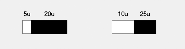
Lotteries will be presented on the screen as shown in the following figure:
Each lottery has two possible prizes, one smaller and one larger, each with an associated probability. These probabilities can be:
 $$20\% ,50\% {\rm{\ or\ }}80\%$$
For each lottery, the probability of winning the smaller prize is indicated by a white bar just below that prize. Likewise, a black bar indicates the probability of winning the larger prize. The probability of getting the larger price is always the complement of the probability of obtaining the smaller one. Therefore, the longer the white bar, the more likely you are to get the smaller prize. And the longer the black bar, the more likely you are to get the larger prize.
In the example displayed in the figure, the left lottery’s smaller prize is 5u, and its associated probability is 20%, therefore the probability of getting the larger prize (20u) is 80%. On the right lottery, the smaller prize is 10u and its probability 50%, so the probability of getting the larger prize (25u) is also 50%.
Once you decide which lottery you want to play by pressing N (left) or M (right), the computer will actually run it, and will calculate the prize according to the specified probabilities. In short, in the example in the figure, if you choose the left lottery (pressing N), you will have a 20% chance of getting 5u and 80% chance of getting 20u. If you choose the right lottery (pressing M), you will have a 50% chance of getting 10u and 50% chance of getting 25u.
Upon choosing, the selected lottery will be highlighted with a red square. The prize corresponding to the outcome of that lottery will be shown shortly afterwards. The value of the prize will appear written in red on the center of the screen. Just to its right, in squared brackets, you will be also shown the prize you did not get from the same lottery. For example, if you choose the left lottery and it turns out that your prize is 5u, the result will be displayed as follows:
 $$\eqalign{ &amp; 5\left[ {20} \right] \cr &amp; {\rm{namely,prize\ won\ }}\left[ {{\rm{prize\ not\ won}}} \right] \cr}$$
Once you have seen the prize won, and the prize not won, resulting from your choice, a second message in blue will appear in the center of the screen. This message will show again the prize you have won and, right next to it, in squared brackets, the prize won by a virtual participant (that is, the computer, which makes decisions according to a pre-programmed algorithm) in that same decision. Therefore, if you have obtained 5u and the virtual counterpart has obtained 10u, you will see a message like this:
 $$\eqalign{ &amp; 5\left[ {10} \right] \cr &amp; {\rm{namely,\ the\ prize\ you\ won\ }}\left[ {{\rm{the\ prize\ won\ by\ the\ computer}}} \right] \cr}$$
This message is only informative, since the computer’s winnings have not any influence on your winnings. The computer will have made its choice between the same two lotteries as you, according to its programmed algorithm. Finally, remember that you will receive payment in real money corresponding to one decision and only one, randomly selected by the computer at the end of the experiment. Thus, your task is to choose the lottery you prefer in every decision, regardless of your choice in the other trials, because only one of them will finally count for the actual payment.
 $${\rm{GOOD\ LUCK}}!$$
Instructions (social conditions): Instructions in the social conditions were mostly equivalent to the ones above, except for the last two paragraphs. In the social-sporadic condition, the corresponding text read as follows.
Once you have seen the prize won, and the prize not won, resulting from your choice, a second message in blue will appear in the center of the screen. This message will show again the prize you have won and, right next to it, in squared brackets, the prize won by another participant in this room on the same decision. Therefore, if you have obtained 5u and the other participant has obtained 10u, you will see a message like this
 $$\eqalign{ &amp; 5\left[ {10} \right] \cr &amp; {\rm{namely,\ the\ prize\ you\ won\ }}\left[ {{\rm{the\ prize\ won\ by\ the\ other\ participant}}} \right] \cr}$$
This message is only informative, since the other person’s winnings have no influence on your winnings. The person whose earnings you will see in blue brackets will be chosen at random in each of the decisions during this experiment (he/she can be any person of this room and he/she will vary in each period). This person will have played the same lotteries at the same time as you. He/she will also be shown your earnings in each trial, in the same way that you see his/hers. Everything is anonymous, so you will never know his/her identity, nor he/she will know yours. Finally, remember that you will receive payment in real money corresponding to one decision and only one, randomly selected by the computer at the end of the experiment. Thus, your task is to choose the lottery you prefer in every decision, regardless of your choice in the other trials, because only one of them will finally count for the actual payment.
Finally, in the social-repeated condition, the corresponding text read as follows.
Once you have seen the prize won, and the prize not won, resulting from your choice, a second message in blue will appear in the center of the screen. This message will show again the prize you have won and, right next to it, in squared brackets, the prize won by another participant in this room on the same decision. Therefore, if you have obtained 5u and the other participant has obtained 10u, you will see a message like this
 $$\eqalign{ &amp; 5\left[ {10} \right] \cr &amp; {\rm{namely,\ the\ prize\ you\ won\ }}\left[ {{\rm{the\ prize\ won\ by\ the\ other\ participant}}} \right] \cr}$$
This message is only informative, since the other person’s winnings have no influence on your winnings. The person whose earnings you will see in blue brackets will be the same for all decisions during this experiment (he/she can be any person of this room and he/she has been chosen at random upon starting). This person will have played the same lotteries at the same time as you. He/she will also be shown your earnings in each trial, in the same way that you see his/hers. Everything is anonymous, so you will never know his/her identity, nor he/she will know yours. Finally, remember that you will receive payment in real money corresponding to one decision and only one, randomly selected by the computer at the end of the experiment. Thus, your task is to choose the lottery you prefer in every decision, regardless of your choice in the other trials, because only one of them will finally count for the actual payment.


