1. INTRODUCTION
Chances matter. My chances of getting cancer influence my decisions about what to eat, how much exercise to do and whether to smoke. The chances of rainfall affect where I choose to holiday. My chances of ‘winning big’ sway my decision for or against entering the National Lottery. These chances matter to me because the things that they are chances-of matter to me. I care about the chances of cancer because I want to avoid cancer, about the chances of rainfall because I prefer to walk in the sunshine, and so on.
How much do chances matter? Or to put the question slightly differently, how much value should we attach to having a chance of a certain magnitude of obtaining some good? In particular, how does it depend on the value of what it is a chance-of? There is a well-established answer to this question, in its contemporary form deriving from the work of von Neumann and Morgenstern on decision making under risk. What von Neumann and Morgenstern’s theory (vN-M for short) tells us, in essence, is that the value of obtaining a chance of a good is a positive linear function of the value of the good. Suppose, for instance, that we are offered the option of a chance x of some good G and that we value G to degree g. Then the vN-M theory tells us to value this option to degree x × g, i.e. that the value of a chance x of G is the value of G discounted by x. The discount reflects the fact that the option does not deliver G with certainty; its magnitude the degree to which the chance of G that it offers falls short of such certainty.
Von Neumann and Morgenstern’s theory is not, of course, restricted in its application to options involving a single outcome. In general it says that the value of an option inducing a probability distribution over a set of mutually exclusive outcomes (a ‘lottery’) is an additive linear function of the probability-utility products of each outcome. The additivity property is controversial however, so I will stick to the simple cases where only one good is at stake. But even for these simple cases, I will argue, the vN-M theory gets it wrong: The value of a chance x of G can permissibly deviate from the x-discounted value of G. My main focus will be on the hypothesis that it is frequently greater than this value, but in principle it can deviate in both directions.
Consider a mountain climber whose enjoyment of climbing partially derives from confronting risk.Footnote 1 For her the activity is of little worth if there is no associated chance of death or injury, even though it is to be avoided if the chances of death or injury are too high. Indeed there is an optimal region of risk, when the chances of death or injury are high enough to require courage of the climber, but not so high as to make the activity foolish. I think that, even if we don’t share the climber’s readiness to embrace risks of this kind, many of us will recognize the contribution that risks of losses or failures makes to the worth of activities we value.
Now the values that the mountain climber puts on the different chances of death and injury are clearly incompatible with the vN-M theory. When the values of the chances of an outcome are a positive linear function of the value of the outcome two things must be the case. Firstly if the outcome has a positive value (i.e. it is a good) then so too must a chance of this outcome and if it has a negative value (it is a bad) then so too must the chance. And secondly, the marginal values of the chances must be constant; for instance, the difference in value between a quarter chance and a half chance must be the same as the difference between a half chance and a three-quarter chance. Neither holds in our example. For the value the mountain climber puts on the chances of death and injury (the bads) are not uniformly negative. And furthermore the marginal values of the chances vary with their magnitude.
The mountain climber is a dramatic example of a commonplace phenomenon: that we value chances of goods non-linearly.Footnote 2 In particular, we very often (permissibly) attach greater value to increases in our chances of a good when they are low than when they are high, a pattern of valuation that implies an aversion to uncertainty about the chances of obtaining a desired good that is analogous to risk aversion with respect to a good like money. The aim of this paper is to show that such aversion to uncertainty about the chances explains a pattern of preferences – ambiguity aversion – that is often observed in the Ellsberg paradox and similar contexts. This pattern is typically taken either to refute Savage’s version of Bayesian decision theory or to be irrational. I shall argue to the contrary: Aversion to uncertainty about the chances of some outcome is a perfectly rational attitude to exhibit and one that is not disallowed by Bayesian decision theory.
This argument hinges on a distinction between the objective chances of some outcome and our subjective beliefs about it and, correspondingly, between the objective and subjective uncertainty we face in our decisions. What exactly objective chances are is a matter of continuing debate in philosophy and not one that I will engage with here. All that matters for the purposes of this paper is that they are features of the world (perhaps frequencies, perhaps the propensities that account for them) rather than properties of the agent’s state of mind, so that it is intelligible that the agent can have beliefs about the chances of events in the same way that she has beliefs about the events themselves. It is true that many well-known Bayesians denied the existence of objective chances, but such metaphysical views are not essential to Bayesian decision theory. In any case what matters from a descriptive point of view is not whether there really are mind-independent chances or not, but whether some agents believe that there are. And of the latter, there is little doubt.
I shall proceed as follows. After presenting the Ellsberg paradox, I will argue that its usual representation is flawed and suggest an alternative. The alternative representation will support the diagnosis that the preference patterns often observed in this context can be attributed to an aversion on the part of agents to uncertainty about the chances of gaining the monetary prizes at stake in the decision problem. Uncertainty aversion, I will argue, is a property of agents’ utility functions for chances of goods that is compatible with Savage’s theory, but only if the vN-M theory is false. In the last section I compare this account of ambiguity aversion to several rival ones, focusing on the theory of Klibanoff et al. (Reference Klibanoff, Marinacci and Mukerji2005).
2. ELLSBERG’S PARADOX
In a justly famous paper on decision making under uncertainty, Ellsberg (Reference Ellsberg1961) presents two experiments that he claims reveal a flaw in Savage’s decision theory. Let us begin by recalling the second of these: the single-urn experiment that is depicted in Table 1. In the set-up Ellsberg describes, an urn is said to contain 90 balls, 30 of which are red, and the remaining 60 are black or yellow in an unknown proportion. Subjects are first asked to choose between two bets. The first, B 1, pays $100 if, in a random draw from the urn, a red ball is drawn. The second, B 2, pays $100 if a black ball is drawn. In a second choice problem, subjects are asked to choose between B 3 and B 4, which respectively pay out $100 in the event of either a red or yellow ball being drawn and in the event of either a black or yellow ball being drawn.
Table 1. The Ellsberg Paradox
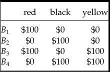
Ellsberg conjectured that many people would express a preference for B 1 over B 2 and for B 4 over B 3. As can easily be verified however, the preferences B 1≻B 2 and B 4≻B 3 are inconsistent with the Bayesian prescription to maximize subjective expected utility (throughout ⪰ and ≻ respectively denote the agent’s weak and strict preferences over options). For whatever probability is assigned to the possible states of the world and whatever utility is assigned to the monetary consequences, the expected utility of B 1 can exceed that of B 2 only if the expected utility of B 3 exceeds that of B 4. Indeed this pattern of preferences – hereafter ‘the Ellsberg preferences ’ – threatens more than one Bayesian principle of rationality. It is evident from the fact that the ‘yellow’ column displays the same consequences for the two pairs of acts, that the Ellsberg preferences violate the Sure-thing principle (Savage’s P2), the requirement that preferences be separable across states of the world. But they are also inconsistent with the way in which subjective probabilities are elicited in Savage’s framework. To see this, note that it follows from Savage’s definition of the qualitative probability relation that B 1≻B 2 iff the event ‘red’ is more probable than the event ‘black’ and that B 4≻B 3 iff the event ‘black or yellow’ is more probable than the event ‘red or yellow’. But the the laws of probability require that ‘red’ is more probable than ‘black’ iff for any event X disjoint with both, ‘red or X’ is more probable than ‘black or X’. Technically, Savage’s axiom of comparative probability (postulate P4) is not violated by the Ellsberg preferences independently of his other postulates. But, as Machina and Schmeidler (Reference Machina and Schmeidler1992) point out, they are inconsistent with a strengthening of it (their ‘strong’ axiom of comparative probability) that is generally taken to be characteristic of probabilistic sophistication, i.e. choice that is based on precise probabilistic beliefs. So it would seem that a Bayesian agent could not display Ellsberg preferences.
2.1. Re-framing Ellsberg’s Problem
Since Ellsberg’s paper there have been numerous experiments reporting patterns of preference akin to those conjectured by Ellsberg, at least in set-ups similar to his.Footnote 3 Ellsberg’s own explanation for these preferences was that agents are averse to what he calls ambiguity, this being the lack of information as to the precise probability distribution over the state space. In the first choice situation in which the subjects find themselves they are given information which makes it reasonable for them to put the probability of drawing a red ball at one-third, but with regard to the probability of a black ball they know only that it is no more than two-thirds. In view of this many people, Ellsberg conjectured, would ‘play it safe’ and opt for the lottery with a known probability of paying out over the one in which there is a good deal of uncertainty about the probability of a win. Similar reasoning would lead them, in the second choice problem, to pick lottery B 4 which has a ‘known’ probability of two-thirds of paying out over B 3 with its ‘unknown’ probability of a win.
Ellsberg’s work has fostered the development of a large number of models of decision making under conditions of ambiguity which relax either the Sure-thing principle or the assumption that individuals are probabilistically sophisticated (or both). But if Ellsberg’s conjecture about how subjects perceive the decision problem they face is correct, then Table 1 does not provide the correct representation of their decision problem. A properly specified decision problem, from Savage’s point of view, is one in which the descriptions of states are maximally specific with regard to the presence or absence of all factors relevant to the determination of consequences that are causally independent of the actions available to the agent, and in which descriptions of consequences are maximally specific with regard to features that matter to the agent’s evaluation of their desirability. Now, on Ellsberg’s analysis, agents have attitudes to the distribution of balls in the urn as well as to the monetary gains attendant on a draw of a ball of a particular colour. This means that strictly speaking the states of the world are not draws of a red, black or yellow ball but combinations of distributions of balls in the urn plus the draw from it; such as ‘The urn contains 30 red balls, 25 black balls and 35 yellow balls. A yellow ball is drawn’ and ‘The urn contains 30 red balls, 60 black balls and no yellow balls. A red ball is drawn’. Together with the chosen act, these two features of the states determine two different features of the consequences; respectively the chances of obtaining the prize and its monetary value.
To determine whether taking into account the distribution from which a ball is drawn makes any difference, we need to draw up the fully refined decision problem. Writing out all the states would be rather tedious however, so I will consider a simple variant of Ellsberg’s set-up in which the urn contains only three balls: One red ball and either two black or two yellow or one of each. This set-up has the same coarse grained representation as Ellsberg’s (i.e. that given by Table 1) but a much simpler refined one, while sharing what seem to be the crucial structural features. So it seems reasonable to presume that agents’ preferences will be the same in the simplified set-up as in the original one (and every model of ambiguity aversion that I know of predicts that they will be).
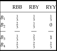
The refined state space in the simplified Ellsberg set-up consists of seven possible states: The possible combinations of distributions of balls and draws of a ball of a particular colour. This suggests a representation as in Table 2, where RBB, RBY and RYY denote the three possible distributions (with, for instance, RBB being the distribution consisting of one red ball and two black balls) and ‘red’, ‘black’ and ‘yellow’ the colour of ball drawn from it.
Table 2. Refined State Space Representation
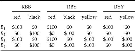
Table 2, unlike Table 1, allows for transparent separation of the agent’s subjective uncertainty regarding the distribution of balls from the objective uncertainty she faces concerning the colour of the ball that will be drawn, given a particular distribution. A number of authors, including Machina (Reference Machina2011), Ergin and Gul (Reference Ergin and Gul2009) and Klibanoff et al. (Reference Klibanoff, Marinacci and Mukerji2005), have exploited this separation to show that there is no incompatibility between the Ellsberg preferences and application of Savage’s axioms to the coarse partition of events {RBB, RBY, RYY}, the domain of her subjective uncertainty.Footnote 4 (This is perhaps evident from the fact that the two pairs of acts, B 1 and B 2, and B 3 and B 4, have different consequences in each coarse state, so that the Sure-thing principle is vacuously satisfied.) And this suggests, as Segal (Reference Segal1990) and others have argued, that ambiguity aversion derives from a failure on the part of the agent to correctly combine subjective and objective uncertainty by reducing the two-tiered state space to a single-tiered one consisting of the seven states (RBB, red), (RBB, black), etc.
As we shall see, this reasoning takes us some, but not all, of the way to the truth. To unpack it further, let us look at a different coarse-grained representation of the simplified Ellsberg set-up, one in which states are individuated by distributions of balls in the urn and consequences are chances of monetary gains. This is illustrated in Table 3 in whose cell entries are the chances of winning $100. Thus an entry of x indicates that making that choice when the world is in that state gives the agent a chance of x of winning $100 and a chance of 1 − x of winning nothing.
Table 3. The Coarser Ellsberg Paradox

Table 3 represents the betting acts B 1 to B 4 as functions from possible ball distributions to chances. Now let us suppose that our agent is a subjective expected utility maximizer à la Savage and moreover that she regards the three possible states of the world as equally likely (perhaps in virtue of symmetry considerations). In this case, a preference for B 1 over B 2 reveals that for the agent, with utility U on the chances of winning $100, it must be the case that ![]() $U(\frac{1}{3})>\frac{1}{3}U(\frac{2}{3})+\frac{1}{3}U(\frac{1}{3})+\frac{1}{3} U(0)$, while a preference for B 4 over B 3 reveals that for the agent
$U(\frac{1}{3})>\frac{1}{3}U(\frac{2}{3})+\frac{1}{3}U(\frac{1}{3})+\frac{1}{3} U(0)$, while a preference for B 4 over B 3 reveals that for the agent ![]() $U(\frac{2}{3})>$
$U(\frac{2}{3})>$![]() $\frac{1}{3}U(\frac{1}{3})+\frac{1}{3}U(\frac{2}{3})+ \frac{1}{3}U(1)$. Together these imply that:
$\frac{1}{3}U(\frac{1}{3})+\frac{1}{3}U(\frac{2}{3})+ \frac{1}{3}U(1)$. Together these imply that:
So we can conclude that an agent who assigns equal probability to the distributions and maximizes subjective expected utility can have Ellsberg preferences over betting acts, provided she values gains in chances of monetary payoffs less as the minimum/maximum chance rises, i.e. if the chances of money have diminishing marginal utility for her. That is to say, contrary to the received view, the Ellsberg preferences are not, on the face of it, ruled out by Bayesian decision theory.
2.2. Ambiguity Aversion
An agent with diminishing marginal utilities for the chances of some good (i.e. with a concave utility function on the chances) will be averse to uncertainty regarding what those chances are. Uncertainty aversion, in the way that I will use the term, is the analogue in contexts where the probabilities of states are not known to the more familiar phenomenon of risk aversion. An agent is canonically said to be risk neutral with respect to some divisible good if she is indifferent between a fixed amount of the good and a lottery which yields the same expected amount of it, but risk averse (loving) if she prefers the former (latter). For instance an agent who is risk averse with regard to money will prefer an act which always pays $50 over one with a 50:50 chance of paying either $100 or nothing. Similarly, someone who is uncertainty averse with respect to some good will prefer acts which yield a constant quantity of the good to those that yield the same expected quantity of it (relative to her subjective probabilities), but have a greater spread.
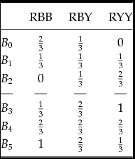
The same applies to someone who is uncertainty averse with respect to the chances of receiving some good (divisible or otherwise). They will prefer acts which yield constant chances of getting the good over acts with the same expected chances when the chances vary by state of the world.Footnote 5 Consider Table 4, for instance, which adds two acts (B 0 and B 5) to the simplified Ellsberg set-up. Someone who regards the distributions RBB and RYY as equiprobable will be indifferent between B 2 and B 0 and between B 3 and B 5. If, furthermore, they are neutral with regard to the chances of monetary gain that are the outcomes of these acts they will regard B 1 as equally good as both B 2 and B 0 and B 4 as equally good as both B 3 and B 5. But if they are uncertainty averse with respect to these chances they will prefer B 1 over the other two because the utility difference between a chance of one-third of the $100 and no chance of it exceeds that between a chance of two-thirds and a chance of one-third. Similarly they will prefer B 4 to both B 3 and B 5.
Table 4. Hedging Acts

Uncertainty attitudes to goods and uncertainty attitudes to the chances of these goods are logically independent. One could be uncertainty neutral with regard to money, but uncertainty averse with respect to the chances of obtaining it. Or just the other way around. But in one crucial respect they are similar: there is nothing particularly rational or irrational about having one uncertainty attitude rather than another.Footnote 6 We certainly do, as a matter of fact, care about the chances of outcomes as well as the outcomes themselves. There is a difference, we tend to think, between having no lottery ticket at all and having a lottery ticket which is not, in fact, a winner. And between succeeding at a task when the chance of doing so was low and succeeding at it when the chance of doing so was very high.
Now agents who are uncertainty averse with respect to the chances of obtaining a good will tend to hedge their chances in the sense of preferring mixtures of equally preferred acts to either of these acts, a pattern of choice that decision theorists, following Schmeidler (Reference Schmeidler1989), regard as the characteristic behavioural property of ambiguity aversion. More formally, let f and g be any two acts whose outcomes are chances of some good. For any α ∈ [0, 1], let the α-mixture of f and g, denoted αf + (1 − α)g, be an act whose consequence in each state of the world, s, is defined by:
Then ambiguity aversion is behaviourally characterized by a preference for an α-mixture of f and g over both f and g, for any acts f and g between which the agent is indifferent. In Table 4, for instance, B 1 can be regarded as an equal weighted mixture of B 2 and B 0, and B 4 as an equal weighted mixture of B 3 and B 5, with mixing producing more constancy in the consequences. And an agent who regards the states RBB, RBY and RYY as equiprobable will be indifferent between B 2 and B 0 and between B 3 and B 5. So ambiguity aversion is revealed by a preference for B 1 over both B 2 and B 0 (and for B 4 over both B 3 and B 5) – just the preference patterns of a chance uncertainty averse expected utility maximizer. The hypothesis of diminishing marginal utility of chances thus affords a Bayesian rationalization of behavioural ambiguity aversion.
2.3. Resolving the ‘Paradox’
The fact that ambiguity aversion is derivable from Savage’s theory together with the hypothesis of chance uncertainty aversion replaces one ‘paradox’ with another. Did we not show in an earlier section that the ambiguity averse preferences of Ellsberg’s subjects were inconsistent with Savage’s postulates? So is the demonstrated compatibility not just an artifice of the re-framing of the decision problem, which succeeds in ‘hiding’ the violation of the Sure-Thing principle ‘evident’ in the framing given by Table 1? To address this challenge, an explanation as to why the two framings of Ellsberg’s set-up lead to different conclusions must be provided.
First, let me concede that for equation (1) not to imply a violation of subjective expected utility theory, it cannot be that, for any chance x of obtaining the $100, U(x) = x · U($100). For were this the case it would follow, in contradiction to equation (1), that:
But this is precisely what is required by Savage’s theory when the decision problem is as represented in either Table 1 or Table 2, i.e. when the consequences are taken to be the monetary prizes. So either these framings are at fault or, contrary to my earlier claim, preferences that are uncertainty averse with respect to chances are not consistent with subjective expected utility theory.
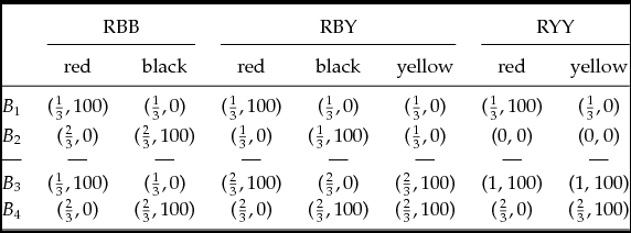
Most decision theorists have taken Table 2, or something much like it, to be the correct fully refined representation of the simplified Ellsberg problem and so have concluded the latter. But the former answer is the correct one. The problem with the framing of the decision problem given in both Table 1 and Table 2 is that the winning of the $100, or otherwise, is not all that matters if agents care about the chances of outcomes as well as the outcomes themselves. Winning nothing when you pick B 1 and a black ball is drawn may not be as bad as winning nothing when you pick B 2 and a yellow ball is drawn. For in the latter case, but not the former, you not only win nothing, but you also had no chance of winning anything. So the significance of winning is different in the two cases. It follows that in the representation given by Table 2, consequences have utilities that are state-dependent. But, as observed earlier, to apply Savage’s theory you must start with descriptions of the states and consequences which are adequate in the sense that they are maximally specific with regard to all that is relevant in determining the outcomes of actions and with regard to all that matters to the agent. So, in particular, consequences in the simplified Ellsberg set-up should be objects of the form ‘Win $100 when the chance of winning is x’ and not simply ‘Win $100’. Footnote 7
The upshot is that a fully refined representation of the decision problem should take the form given by Table 5, not Table 2. In this representation the consequences are given by pairs of the form (x, $y) where x is the chance of obtaining the $100 and y the amount of money actually won. Once consequences are properly described, the apparent inconsistency between subjective expected utility theory and the Ellsberg preferences found in Table 2 disappears. In particular, it is evident that there is no violation of the Sure-thing principle as the (RYY, yellow) column displays different chance-consequences for each act.
Table 5. Fully Refined Ellsberg Problem

3. A TRILEMMA FOR DECISION THEORY
Ellsberg’s experiments, and others like it, provide strong evidence that at least some people are ambiguity averse in some contexts. This fact creates an explanatory trilemma for normative decision theory. As we have just seen, ambiguity aversion can be explained by aversion to uncertainty about chances, a rationally permissible property of the agent’s utility function that is perfectly consistent with Savage’s theory. However, since chance uncertainty aversion is not compatible with the vN-M theory (because, as we saw earlier, if the value of a chance of good is a linear function of the chance, then the chances must have constant marginal utility), the price of saving Savage’s theory in this way, is that the vN-M theory must be rejected. Alternatively ambiguity aversion can be explained in a manner consistent with the vN-M theory, but at the price of rejecting Savage’s theory as the correct normative account of decision making under subjective uncertainty. Finally, one can retain the theories of both Savage and vN-M, but at the price of accepting that the Ellsberg preferences are irrational. Most decision theorists ‘grasp’ either the second or third horn of this trilemma. Here I have argued for accepting the first.
An important, if somewhat technical, qualification: Rejection of the vN-M theory does not entail rejection of the vN-M axioms of preference over lotteries. These axioms imply the existence of an expected utility representation of preference, unique up to affine transformation, but unique as a type of representation only up to positive monotone transformation. In the simple case to which we restricted ourselves where there is only one good G, lotteries are just chances of G, and the vN-M theory says that rational preference for these lotteries is represented by a function EU on chances of G such that EU(x) = x, for any chance x of G. But then any positive monotone transformation of EU also ordinally represents these preferences. In particular, let ϕ(EU) be a concave transformation of EU. It too represents the preferences of an agent who satisfies the vN-M axioms, but does so in a way which encodes chance uncertainty aversion. So these axioms do not settle the question of whether EU or ϕ(EU) is the correct measure of the agent’s degrees of preference and hence whether chance uncertainty neutrality is a requirement of rationality. When only preferences amongst risky options are at stake there is perhaps no meaningful way of settling the issue (or, for that matter, any point in doing so), but when we widen consideration to uncertain options the situation changes. Whereas the hypotheses that, respectively, EU or ϕ(EU) is the correct measure of the agent’s degrees of preference, are observationally equivalent with respect to her choices amongst lotteries, these hypotheses conjoined with Bayesian decision theory are not observationally equivalent with respect to her choices amongst acts with consequences that are objective chances of goods.
To explore the trilemma more formally, let us state things within a framework akin to the Anscombe and Aumann (Reference Anscombe and Aumann1963) one in which much of the economics literature on ambiguity attitudes is couched. Let Pr be a measure of the agent’s degrees of belief on a set of states ![]() $\mathcal {S} =\lbrace s_{i}\rbrace$ and let acts be functions from states of the world to consequences, which in this context are just the chances of gaining some good G. Recall that the vN-M theory says that the value of these chances is measured by a function EU, such that EU(x) = x.U(G), for any chance x of G. Then on the theory I am advocating the function V on acts such that, for any act f,
$\mathcal {S} =\lbrace s_{i}\rbrace$ and let acts be functions from states of the world to consequences, which in this context are just the chances of gaining some good G. Recall that the vN-M theory says that the value of these chances is measured by a function EU, such that EU(x) = x.U(G), for any chance x of G. Then on the theory I am advocating the function V on acts such that, for any act f,
is a subjective expected utility representation of the preferences of a rational agent, with ϕ a transformation of the chances (thus of EU, the vN-M utility on chances) that represents her uncertainty attitudes to them. In particular ϕ is linear for chance uncertainty neutral agents, but concave for those that are uncertainty averse.
The function V is an expectation based on (subjective) probabilities for (objective) probabilities – the chances of the good – with the notable feature that the two tiers of probability are not reducible to a single expectation for the good. As mentioned before, this is a feature of a number of models of ambiguity aversion to be found in the literature, including those of Segal (Reference Segal1990), Klibanoff et al. (Reference Klibanoff, Marinacci and Mukerji2005), Seo (Reference Seo2009) and Ergin and Gul (Reference Ergin and Gul2009). In particular, formally speaking (and setting aside small differences in vocabulary) our theory is just the special case of the smooth ambiguity model of Klibanoff, Marinacci and Mukerji (KMM for short) that is obtained when it is restricted to single-good lotteries. (In their more general model, ϕ is a transformation, not of the utility of chances, but of an expected utility representation of the agent’s preferences over lotteries; a natural generalization of equation (3), at least when only a single type of good is at stake.)
Where we differ is on the interpretation of the model. KMM seem to view the function EU (more generally, vN-M expected utility) as an appropriate measure of the desirability of chances (more generally, of lotteries) and ϕ as a transformation induced by the kind of epistemic attitude that Ellsberg postulated: A dislike of lack of information that distorts the subjective probabilistic weighting of outcomes. I view ϕ(EU) itself as the correct measure of the desirability of the lotteries, with ϕ a pragmatic attitude to uncertainty about chances that is encoded in the concavity of the utility function for chances. Finally Seo offers a formulation in which ϕ encodes a failure to reduce two-stage lotteries. So adoption of a model based on equation (3) returns us to the explanatory trilemma, now focused on the interpretation of the function ϕ, with the alternatives of rejecting Savage, vN-M, or the rationality of the Ellsberg preferences.
It is beyond the scope of this paper to consider in full the pros and cons of each interpretation. But I will finish by looking at two issues that shed light on the relative merits of the KMM interpretation and the one defended here.
3.1. Chances of Losses
Let’s begin with the explanatory adequacy of the two accounts of behavioural ambiguity aversion. Ellsberg’s explanation of it in terms of a dislike of lack of information has, for the most part, been accepted in the literature, but the evidence considered so far is not in fact sufficient to distinguish this explanation from one in terms of chance uncertainty aversion. The two hypotheses will have different implications for predictions of behaviour in other domains however. If it is the dislike of lack of information that motivates agents, then we should expect to see ambiguity aversion to much the same extent in choices between acts yielding other outcomes than the monetary gains considered so far, so long as the same lack of information is involved. On the other hand, if it is the value that agents place on the chances of obtaining goods that motivates them, then the type of good involved will quite plausibly make a difference. Agents may well, for instance, value chances of goods like health and education differently from money in much the same way as they value the goods themselves differently.
To take a particular example, let’s consider a choice between acts that involve chances of losses rather than gains. Such a decision problem, the negative image of the Ellsberg paradox, is displayed in Table 6. In this set-up agents must choose between lotteries that yield losses of $100 or $0, contingent on the colour of a ball drawn from the same urn as in the standard Ellsberg set-up, i.e. one containing one-third red balls and the rest black or yellow.
Table 6. The Negative Ellsberg Problem
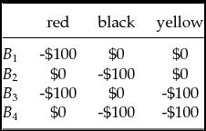
If individuals are ambiguity averse due to a preference for lotteries in which the chances of the outcomes are known over those in which they are not, then they will exhibit the same pattern of preferences in the Negative Ellsberg problem as they do in the standard Ellsberg set-up, namely B 1⪰B 2 and B 4⪰B 3. The empirical data on this question are fairly sparse, but on the whole do not support this prediction. Abdellaoui et al. (Reference Abdellaoui, Vossmann and Weber2005) and Trautmann et al. (Reference Trautmann, Vieider and Wakker2011), for instance, all report ambiguity aversion in choice experiments involving monetary gains, but ambiguity seeking behaviour in those involving monetary losses.Footnote 8
Such a reversal of the Ellsberg preferences is hard to explain in terms of aversion to lack of information. But they are hardly surprising if it is correct that the chances themselves matter. For why should we not value gains and losses in chances differently depending on what our reference point for these changes are (our initial chance endowment), just as we value gains and losses of money and other goods differently depending on our initial endowment? Indeed if our uncertainty attitudes to the chances of outcomes match our uncertainty attitudes to the outcomes themselves, then the fact that agents are often mildly uncertainty loving with regard to monetary losses would suggest similar uncertainty loving attitudes towards chances of monetary losses. So the hypothesis that agents have pragmatic attitudes to uncertainty about chances furnishes the possibility of explaining the reversal of the typical Ellsberg preferences in the domain of monetary losses.
3.2. Epstein’s Paradox
In this final subsection I want to consider the implications of an objection to Klibanoff et al.'s (Reference Klibanoff, Marinacci and Mukerji2005) smooth ambiguity model raised by Larry Epstein (Reference Epstein2010). KMM assume that rational agents are vN-M expected utility maximizers over lotteries (and hence in particular on the chances of some good) and Savage subjective expected utility maximizers over the space of acts with non-risky consequences that they call ‘second-order’ acts. (Second-order acts are important to their account because they allow for the identification of the agent’s beliefs about the objective chances.)
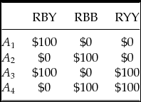
Consider Table 7 which represents a decision problem involving the second-order acts associated with the simplified Ellsberg paradox, with the states of the world corresponding to the distributions of balls and monetary consequences representing the prizes for correctly identifying which distribution is the true one. Thus act A 1 pays out when there is one ball of each colour, A 2 when there are two black balls in addition to the red, and so on.
Table 7. The Epstein Paradox

Suppose that the distribution of balls is generated in the following way. An urn (the ‘second-order’ urn) is filled with three balls, one of which is red and the other two are either black or yellow, and a ball is drawn at random. If the red ball is drawn then the Ellsberg ‘first-order’ urn is made up as RBY, if black is drawn then it is made up as RBB and if yellow is drawn then it is RYY. In the light of this the decision problem represented by Table 7 is structurally identical to the Ellsberg problem in that the consequence matrix is the same and we hold the same information about the states, namely that RBY has an objective probability of one-third, while both RBB and RYY have probabilities between zero and two-thirds. Hence, Epstein argues, rational agents should exhibit exactly the same pattern of preferences, namely A 1≻A 2 and A 4≻A 3. But this is contrary to the assumption of KMM that preferences over second-order acts should respect the Savage axioms.
Klibanoff et al. (Reference Klibanoff, Marinacci and Mukerji2012) respond to Epstein by arguing that his representation of his problem is inadequate and that once consideration is given to all probability distributions over the contents of both urns, then the smooth ambiguity model predicts the same preference pattern in Epstein’s set-up as in Ellsberg’s. But this reply strikes me as unconvincing. Firstly, it somewhat misses the essential point of Epstein’s paradox, namely that the smooth ambiguity model does not allow for ambiguity aversion when the agent is simply betting on what the chances are (i.e. when she is choosing amongst second-order acts). His introduction of a second-order urn was presumably motivated simply by the desire to make concrete the truth-conditions for these chances.
Secondly, it seems to me that the prediction that Epstein attributes to the KMM theory in his problem is in fact the correct prediction to make. For Table 7 is not structurally identical to the Ellsberg problem when the latter is properly represented as in Table 5. In the Ellsberg problem, chances are relevant not just as determinants of the monetary payoffs, but also as consequences. In Epstein’s problem, on the other hand, the chances are not at stake for the agent, for they are not determined by their choice of action. Or to put it slightly differently, whereas in Epstein’s problem there is ambiguity, in the sense of lack of information about the chances, but no grounds for chance uncertainty aversion, in Ellsberg’s problem both are present. So we should expect ambiguity aversion only in the latter case.
Epstein’s example poses a difficult challenge for the KMM theory. On the one hand, their theory (and equation (3) in particular) prescribes different choices in the Epstein and Ellsberg paradoxes; on the other hand, if ambiguity aversion is an attitude to absence of information one would expect the same choices in both. But if ambiguity aversion is viewed as a pragmatic attitude to chances, the challenge is easily met. So chance uncertainty aversion provides a better interpretation of their theory than the one that KMM adopts; an interpretation that resolves both the Ellsberg and Epstein paradoxes.
4. CONCLUSION
I have argued that, contrary to the vN-M theory, we value the chances of goods non-linearly and in particular that increases in our chances of a good are more valuable when they are low than when they are high. This uncertainty aversion with respect to chances provides an explanation of the patterns of behaviour typically observed in the Ellsberg paradox. Moreover it is an explanation that is consistent with the theory of subjective expected utility maximization due to Savage. This should not be taken to be blanket endorsement of Savage’s theory. There are many situations in which we are unable to assign probabilities to all relevant contingencies and in which Savage’s theory will not apply. But the Ellsberg set-up is not one of them. Its lesson is not that rationality does not require probabilistic sophistication, but rather that rationality does not require uncertainty neutrality with respect to chances.
ACKNOWLEDGEMENTS
I am very grateful to Suzanne Burri, Hilary Greaves, Alex Voorhoeve, Ittay Nissan, Orri Stefánsson and two anonymous referees for Economics and Philosophy for their comments on earlier drafts, as well as the audiences of the LSE Choice Group Seminars and the EIPE Research Seminars and the participants in the Conference on Rational Choice and Philosophy at Vanderbilt University. The research for this paper was supported by the Arts and Humanities Research Council (grant reference: AH/J006033/1).

