


1 Introduction
At high Reynolds number, the turbulent boundary layer is composed of large uniform momentum zones (UMZs) segregated by narrow regions of high shear, i.e. vortical fissures (VFs), which are largely responsible for the momentum exchange (Meinhart & Adrian Reference Meinhart and Adrian1995; Priyadarshana et al. Reference Priyadarshana, Klewicki, Treat and Foss2007). This binary UMZ/VF structure suggests a simple representation of streamwise velocity fluctuations in the inertial region of the turbulent boundary layer. The authors recently developed and validated a one-dimensional model of the UMZ/VF structure of the streamwise velocity fluctuations (Cuevas Bautista et al. Reference Cuevas Bautista, Ebadi, White, Chini and Klewicki2019) based on the analysis of the mean streamwise momentum equation (Wei et al. Reference Wei, Fife, Klewicki and McMurtry2005a; Klewicki et al. Reference Klewicki, Philip, Marusic, Chauhan and Morrill-Winter2014).
Recent studies suggest that large-scale motions within the UMZs strongly influence the transport of passive scalars in the turbulent boundary layer (Finnigan, Shaw & Patton Reference Finnigan, Shaw and Patton2009; Michioka & Sato Reference Michioka and Sato2012; Perret & Savory Reference Perret and Savory2013; Vanderwel & Tavoularis Reference Vanderwel and Tavoularis2016; Eisma Reference Eisma2017). Using large-eddy simulation (LES), Finnigan et al. (Reference Finnigan, Shaw and Patton2009) provided evidence of zones of high concentration gradients above a vegetation canopy (namely, microfronts). Michioka & Sato (Reference Michioka and Sato2012) investigated the effects of coherent structures on pollutant removal from an idealized canyon using LES. They found that coherent structures of low-momentum fluid contribute to pollutant removal, with the removal being directly related to the size of the coherent structures. Vanderwel & Tavoularis (Reference Vanderwel and Tavoularis2016) studied the dynamics of coherent structures as a mechanism for scalar dispersion. They found hairpin vortices to be responsible for the large scalar flux and Reynolds stress events in the flow.
Other studies exploring the topology of the temperature field in a turbulent flow compared the statistical features of the momentum and temperature field probability density functions (PDFs), seeking to confirm the universality of the small scales (for example, Sreenivasan et al. (Reference Sreenivasan, Hunt, Phillips and Williams1991)). Examination of the time series of the temperature fluctuations reveals a characteristics ramp–cliff structure, in which a long gradual increase in the temperature (the ramp) is followed by a short steep decrease in the temperature (the cliff) (Sreenivasan, Antonia & Britz Reference Sreenivasan, Antonia and Britz1979; Shraiman & Siggia Reference Shraiman and Siggia2006; Wroblewski et al. Reference Wroblewski, Coté, Hacker and Dobosy2007).
The above studies indicate a number of mechanisms that may relate the passive scalar transport to the dynamics of the momentum field. The present work focuses on recent studies in canonical smooth-wall flows, in which the momentum and passive scalar fields exhibit similar binary structures (extended regions of uniform quantity segregated by narrow regions of large gradient). In particular, Eisma (Reference Eisma2017) performed time-resolved tomographic particle image velocimetry (TPIV) and laser-induced fluorescence (LIF) to study the role of UMZs and VFs on the dispersion of a passive scalar. Their analysis of the PDFs of the experimentally acquired instantaneous velocity and concentration fields revealed the coexistence of UMZs, and what they termed uniform concentration zones (UCZs). Along with describing the geometrical characteristics of the zones and quantifying the overlap between the UMZs and UCZs, Eisma (Reference Eisma2017) proposed a first-order jump model for the transport of scalar concentration, similar to that for the transport of the momentum field.
Motivated by the similarities in the equations governing the transport of momentum and passive scalars, and by the analogous binary structures of the two fields, we construct and validate a simple one-dimensional heat transfer model of fully developed turbulent channel flow (the passive scalar field in the present work is represented by temperature). The theoretical basis of the model is founded on the asymptotic scaling structure of turbulent channel flow as determined by analysis of the mean equations (Wei et al. Reference Wei, Fife, Klewicki and McMurtry2005b; Zhou, Pirozzoli & Klewicki Reference Zhou, Pirozzoli and Klewicki2017). Informed specifically by analysis of the passive scalar transport equation, the inertial domain of the boundary layer is modelled as comprising large uniform temperature zones (UTZs) separated by narrow regions of high gradient, i.e. thermal fissures (TFs). The most probable location and the characteristic scalar value of the UTZs are determined by the analysis of the mean scalar transport equation. The UTZ/TF model is then extended to the subinertial domain, within which the characteristics of the UTZs are empirically determined. The statistical profiles generated by the model are in good agreement with the direct numerical simulation (DNS) data for a range of Prandtl ( $Pr$) numbers. Furthermore, the streamwise turbulent heat flux is accurately reproduced by integrating the UMZ/VF and the UTZ/TF models. Lastly, the
  $Pr$-dependency of the empirically chosen model parameters is investigated.
In the next section, a brief overview of the model basis is provided. In § 3, the model construction and algorithm are described. The statistical profiles generated by the model are then compared to DNS data at a friction Reynolds number  $\unicode[STIX]{x1D6FF}^{+}=4088$ for different
  $Pr$ (Pirozzoli, Bernardini & Orlandi Reference Pirozzoli, Bernardini and Orlandi2016), where
  $\unicode[STIX]{x1D6FF}^{+}=u_{\unicode[STIX]{x1D70F}}h/\unicode[STIX]{x1D708}$,
  $h$ is the channel half-height,
  $\unicode[STIX]{x1D708}$ is the kinematic viscosity,
  $u_{\unicode[STIX]{x1D70F}}=\sqrt{\unicode[STIX]{x1D70F}_{w}/\unicode[STIX]{x1D70C}}$ is the friction velocity,
  $\unicode[STIX]{x1D70C}$ is the density and
  $\unicode[STIX]{x1D70F}_{w}$ is the wall shear stress. The DNS conducted by Pirozzoli et al. (Reference Pirozzoli, Bernardini and Orlandi2016) incorporate a constant heat generation term in the scalar transport equation. For more details on the simulation set-up, grid allocation and mesh convergence the reader is referred to Pirozzoli et al. (Reference Pirozzoli, Bernardini and Orlandi2016). Lastly, a rudimentary sensitivity analysis of the model parameters to variations in
  $Pr$ is performed.
2 Model basis
The current model is founded on the self-similar thermal structure of fully developed channel flow with uniform heat generation and fixed (and equal) lower and upper wall temperatures previously analysed and determined by Zhou et al. (Reference Zhou, Pirozzoli and Klewicki2017). Under these conditions, the mean scalar transport equation reduces to a form analogous to the mean momentum equation,
 $$\begin{eqnarray}\unicode[STIX]{x1D6FC}\frac{\text{d}^{2}\unicode[STIX]{x1D6E9}}{\text{d}y^{2}}-\frac{\text{d}\overline{v^{\prime }\unicode[STIX]{x1D703}^{\prime }}}{\text{d}y}+Q=0,\end{eqnarray}$$
 where  $\unicode[STIX]{x1D6FC}$ is the thermal diffusivity,
  $y$ is the wall-normal direction,
  $\unicode[STIX]{x1D6E9}$ and
  $\unicode[STIX]{x1D703}^{\prime }$ are the mean and fluctuating temperature, respectively,
  $v^{\prime }$ is the fluctuating wall-normal velocity and
  $Q$ is the uniform volumetric heat generation. Assuming statistical symmetry about the channel centreline and using
  $-\overline{v^{\prime }\unicode[STIX]{x1D703}^{\prime }}|_{wall}=0$, it can be shown analytically that
 $$\begin{eqnarray}Q=\frac{\unicode[STIX]{x1D703}_{\unicode[STIX]{x1D70F}}u_{\unicode[STIX]{x1D70F}}}{h},\end{eqnarray}$$
 where  $\unicode[STIX]{x1D703}_{\unicode[STIX]{x1D70F}}=(\unicode[STIX]{x1D6FC}/u_{\unicode[STIX]{x1D70F}})(\text{d}\unicode[STIX]{x1D6E9}/\text{d}y)|_{wall}$ is the friction temperature. Normalizing (2.1) using wall units yields
 $$\begin{eqnarray}\underbrace{\frac{1}{Pr}\frac{\text{d}^{2}\unicode[STIX]{x1D6E9}^{+}}{\text{d}y^{+2}}}_{MD}+\underbrace{\frac{\text{d}T_{\unicode[STIX]{x1D703}}^{+}}{\text{d}y^{+}}}_{GT}+\underbrace{\frac{1}{\unicode[STIX]{x1D6FF}^{+}}}_{HG}=0,\end{eqnarray}$$
 where  $Pr=\unicode[STIX]{x1D708}/\unicode[STIX]{x1D6FC}$ is the Prandtl number and
  $T_{\unicode[STIX]{x1D703}}^{+}=-\overline{v^{\prime }\unicode[STIX]{x1D703}^{\prime }}^{+}$. The three terms in (2.3) from left to right are the molecular diffusion (
 $MD$), gradient of the wall-normal turbulent heat flux (
 $GT$) and heat generation (
 $HG$). Following the work of Wei et al. (Reference Wei, Fife, Klewicki and McMurtry2005a), who investigated the balance of the leading-order terms in the mean momentum equation, Zhou et al. (Reference Zhou, Pirozzoli and Klewicki2017) explored the balance of the leading-order terms in (2.3) by studying the ratio
  $MD/GT$. They identified four distinct layers, in which
  $GT$,
$GT$,  $HG$ and
  $MD$ are, respectively, subdominant in layers I, II and IV. In layer III, however, all three terms are comparable in magnitude.
Analysis of the mean scalar transport equation reveals the existence of a self-similar hierarchy of layers, on which the mean equation can be continuously rescaled into a single parameter-free form with all three terms retaining leading-order significance. The width  $W_{\unicode[STIX]{x1D703}}$ of each layer of the hierarchy, which is the characteristic length scale for the rescaling, is the average size of the turbulent motions responsible for the net flux of heat towards the wall, where in wall units
  $W_{\unicode[STIX]{x1D703}}^{+}=(-\text{d}^{2}\unicode[STIX]{x1D6E9}^{+}/\text{d}y^{+2})^{-1/2}$ (Zhou et al. Reference Zhou, Pirozzoli and Klewicki2017). In the present study a UTZ and its adjacent TF are interpreted as one layer in the hierarchy. Figure 1 plots the distribution of hierarchy layer widths. As evident from the plot,
  $W_{\unicode[STIX]{x1D703}}^{+}$ is approximately a linear function of
  $y^{+}$ in layer IV (non-diffusive domain), such that
  $\text{d}W_{\unicode[STIX]{x1D703}}^{+}/\text{d}y^{+}=1/\unicode[STIX]{x1D719}_{\unicode[STIX]{x1D703}c}$ can be identified, where
  $\unicode[STIX]{x1D719}_{\unicode[STIX]{x1D703}c}^{2}=1/\unicode[STIX]{x1D705}_{\unicode[STIX]{x1D703}}$ (
 $\unicode[STIX]{x1D705}_{\unicode[STIX]{x1D703}}$ is the scalar Karman constant). This formulation directly leads to a log law by integrating the mean equation. Following the same methodology used in the study of the dynamical self-similar hierarchy (Klewicki et al. Reference Klewicki, Philip, Marusic, Chauhan and Morrill-Winter2014; Cuevas Bautista et al. Reference Cuevas Bautista, Ebadi, White, Chini and Klewicki2019), a discrete version of the hierarchy layer structure in layer IV can be developed. The wall-normal distance (
 $\unicode[STIX]{x0394}y^{+}$) and the mean temperature increment (
 $\unicode[STIX]{x0394}\unicode[STIX]{x1D6E9}^{+}$) from the
  $i$th layer to the next (
 $i+1$) can be estimated by
 $$\begin{eqnarray}\unicode[STIX]{x0394}y^{+}\equiv y_{i+1}^{+}-y_{i}^{+}\approx \frac{\unicode[STIX]{x1D719}_{\unicode[STIX]{x1D703}c}+1}{\unicode[STIX]{x1D719}_{\unicode[STIX]{x1D703}c}}y_{i}^{+}\end{eqnarray}$$
and
 $$\begin{eqnarray}\unicode[STIX]{x0394}\unicode[STIX]{x1D6E9}^{+}\equiv \unicode[STIX]{x1D6E9}_{i+1}^{+}-\unicode[STIX]{x1D6E9}_{i}^{+}\approx \unicode[STIX]{x1D719}_{\unicode[STIX]{x1D703}c}^{2}\ln \left(\frac{\unicode[STIX]{x1D719}_{\unicode[STIX]{x1D703}c}+1}{\unicode[STIX]{x1D719}_{\unicode[STIX]{x1D703}c}}\right)\end{eqnarray}$$
 for non-negative integer  $i$. The details of the analogous dynamical hierarchy discretization can be found in Cuevas Bautista et al. (Reference Cuevas Bautista, Ebadi, White, Chini and Klewicki2019).

Figure 1. Distribution of  $W_{\unicode[STIX]{x1D703}}^{+}$ for (a)
  $Pr=0.2$ with dashed line:
  $\unicode[STIX]{x1D6FF}^{+}=548$, dashed-dotted line:
  $\unicode[STIX]{x1D6FF}^{+}=995$, dotted line:
  $\unicode[STIX]{x1D6FF}^{+}=2017$, and solid line:
  $\unicode[STIX]{x1D6FF}^{+}=4088$; (b)
  $\unicode[STIX]{x1D6FF}^{+}=4088$ with solid line:
  $Pr=0.20$, dashed line:
  $Pr=0.71$, dotted line:
  $Pr=1$. The dashed vertical lines denote the lower bound of layer IV for
  $\unicode[STIX]{x1D6FF}^{+}=4088$ and
  $Pr=1$.
3 Model construction
Considering analogous equations and hierarchical layer structures, the present model is constructed similarly to the UMZ/VF model of Cuevas Bautista et al. (Reference Cuevas Bautista, Ebadi, White, Chini and Klewicki2019). In the current model a finite number of TFs ( $n_{TF}+N_{TF}$, where
  $n_{TF}$ and
  $N_{TF}$ are the number of subinertial and inertial TFs, respectively) are positioned across the channel to create a master profile using the UTZ/TF thesis. This master profile represents the most probable arrangement of the TFs and serves as the baseline from which instantaneous temperature profiles are generated by repositioning the TFs. This process is repeated to create an ensemble of instantaneous temperature profiles, from which statistical moments are calculated.
In what follows, the formulation of the UTZ/TF model, including the rationale for the number of TFs, their most probable positions, and the perturbation procedure, is briefly described. The discussion is separated into two parts. First, the inertial-layer (non-diffusive domain) formulation, which is based on the analysis summarized in § 2, is described. Then the subinertial layer (diffusive domain) formulation is described. The empirical parameters used in the construction of the model are adapted from Cuevas Bautista et al. (Reference Cuevas Bautista, Ebadi, White, Chini and Klewicki2019).
3.1 Inertial domain UTZ/TF model
Based upon the UMZ/VF model, the centroid of the first (lowest) inertial domain TF in the master profile is placed at the lower edge of layer IV (i.e.  $y_{n_{VF}+1}^{+}=2.5\sqrt{\unicode[STIX]{x1D6FF}^{+}/Pr}$) with
  $\unicode[STIX]{x1D6E9}_{n_{TF}+1}^{+}=\unicode[STIX]{x0394}\unicode[STIX]{x1D6E9}_{I}^{+}+\unicode[STIX]{x0394}\unicode[STIX]{x1D6E9}_{II}^{+}+\unicode[STIX]{x0394}\unicode[STIX]{x1D6E9}_{III}^{+}$, where
  $\unicode[STIX]{x0394}\unicode[STIX]{x1D6E9}_{I}$,
  $\unicode[STIX]{x0394}\unicode[STIX]{x1D6E9}_{II}$ and
  $\unicode[STIX]{x0394}\unicode[STIX]{x1D6E9}_{III}$ are the mean temperature increments across layers I, II and III, respectively. The mean temperature increments, which all attain constancy as
  $\unicode[STIX]{x1D6FF}^{+}\rightarrow \infty$, are adopted from Zhou et al. (Reference Zhou, Pirozzoli and Klewicki2017). The rest of the TFs in the inertial domain are placed according to (2.4) and (2.5). Using (2.4) and imposing
  $y_{n_{TF}+N_{TF}}^{+}\leqslant \unicode[STIX]{x1D6FF}^{+}$, the number of TFs in layer IV can be approximated by
  $N_{TF}\approx \lfloor \ln (Pr\unicode[STIX]{x1D6FF}^{+})-0.8\rfloor$, where
  $\lfloor \bullet \rfloor$ is the floor function. The UTZ/TF model does not specify the width
  $f_{w}$ or the temperature profile within a TF. Similar to the dynamical hierarchy,
  $f_{w}^{+}\approx \sqrt{\unicode[STIX]{x1D6FF}^{+}/Pr}$ is predicted for the TFs in the inertial domain (Klewicki Reference Klewicki2013; Zhou et al. Reference Zhou, Pirozzoli and Klewicki2017). We investigated the model results for various values of
  $f_{w}^{+}$, ranging from 2 to
  $\sqrt{\unicode[STIX]{x1D6FF}^{+}/Pr}$, and the comparison of the statistical moments confirms that the model is independent of
  $f_{w}^{+}$ over this range in the inertial region, where the molecular diffusivity is negligible. Therefore, a width
  $f_{w}^{+}=6$ (this choice is justified in the later sections) and a linear temperature profile within the TFs are prescribed. The lower and upper edge temperatures of the TFs are then defined as follows:
 $$\begin{eqnarray}\displaystyle & \unicode[STIX]{x1D6E9}_{i,low}^{+}={\textstyle \frac{1}{2}}(\unicode[STIX]{x1D6E9}_{i}^{+}+\unicode[STIX]{x1D6E9}_{i-1}^{+}), & \displaystyle\end{eqnarray}$$
 $$\begin{eqnarray}\displaystyle & \unicode[STIX]{x1D6E9}_{i,up}^{+}={\textstyle \frac{1}{2}}(\unicode[STIX]{x1D6E9}_{i}^{+}+\unicode[STIX]{x1D6E9}_{i+1}^{+}). & \displaystyle\end{eqnarray}$$
3.2 Subinertial domain UTZ/TF model
While DNS supports the existence of staircase-like structure of instantaneous streamwise velocity and temperature in the subinertial domain (see figure 3), unlike the inertial domain, the  $W_{\unicode[STIX]{x1D703}}^{+}$ profile in the subinertial domain (
 $y^{+}\leqslant 2.5\sqrt{\unicode[STIX]{x1D6FF}^{+}/Pr}$) is not linear. Hence, the analytical foundations of the current UTZ/TF model given in § 2 cannot be extended to the subinertial domain, in which the molecular diffusion is not negligible. Nevertheless, the nonlinear
  $W_{\unicode[STIX]{x1D703}}^{+}$ profile in the subinertial domain exhibits an invariant form for a given
  $Pr$, i.e. the profile does not vary with
  $\unicode[STIX]{x1D6FF}^{+}$ (figure 1a). Following Cuevas Bautista et al. (Reference Cuevas Bautista, Ebadi, White, Chini and Klewicki2019), a surrogate parameter
  $\tilde{\unicode[STIX]{x1D719}_{\unicode[STIX]{x1D703}}}$ is defined as follows:
 $$\begin{eqnarray}\unicode[STIX]{x1D6E9}_{i+1}^{+}=\unicode[STIX]{x1D6E9}_{i}^{+}+\tilde{\unicode[STIX]{x1D719}_{\unicode[STIX]{x1D703}}}(y_{i}^{+})^{2}\ln (y_{i+1}^{+}/y_{i}^{+}).\end{eqnarray}$$
 The surrogate parameter is approximated by fitting a curve to the DNS data so that an analytical approximation to  $W_{\unicode[STIX]{x1D703}}^{+}$ in the subinertial domain can be obtained. The subinertial TFs in the master profile are logarithmically allocated and their corresponding temperature increments are then determined by (3.3). Unlike in the inertial domain, the width of the TF has a significant impact on the statistical profiles near the wall. Based on a posteriori comparisons,
  $f_{w}^{+}=6$ produces the most accurate results in the subinertial domain. Thus, for simplicity,
  $f_{w}^{+}=6$ is prescribed uniformly for the entire channel. Lastly, similar to the inertial domain, a linear temperature profile within the TFs is prescribed. Figure 2 compares the master profiles of velocity and temperature predicted by the UMZ/VF and UTZ/TF models, respectively, for given Reynolds and Prandtl numbers. Once the master profile is formed, the positions and the temperatures of the TF centroids are perturbed, following the protocol described in the next subsection, to generate statistically independent ensembles.

Figure 2. Discrete master temperature (solid lines) and velocity (dashed lines) profiles predicted by the present and UMZ/VF models, respectively, for  $\unicode[STIX]{x1D6FF}^{+}=4088$ and
  $Pr=1$.

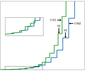
Figure 3. Instantaneous temperature (a) and velocity (b) profiles acquired simultaneously for  $Pr=1$ at
  $\unicode[STIX]{x1D6FF}^{+}=4088$. The horizontal dashed lines show the lower limit of the inertial layers and subscripts
  $w$ and
  $CL$ denote the magnitude at the wall and centreline, respectively. The pink regions indicate the thermal (a) and vortical (b) fissures in the subinertial region, where the labels correspond to the centre location of the fissure. These fissures are identified by a gradient threshold method.

Figure 4. Statistical moments of the passive scalar computed using the UTZ/TF model (–●–) for  $Pr=0.2$ (
 $a$),
$a$),  $Pr=0.71$ (
 $b$) and
  $Pr=1.0$ (
 $c$) at
  $\unicode[STIX]{x1D6FF}^{+}=4088$. The profiles in each row are the mean temperature
  $\unicode[STIX]{x1D6E9}^{+}$, variance
  $\overline{\unicode[STIX]{x1D703}^{^{\prime }2}}^{+}$, skewness
  $S(\unicode[STIX]{x1D703}^{\prime })$ and kurtosis
  $K(\unicode[STIX]{x1D703}^{\prime })$ of the scalar field fluctuations
  $\unicode[STIX]{x1D703}^{\prime }$, and the streamwise turbulent heat flux
  $\overline{u^{\prime }\unicode[STIX]{x1D703}^{\prime }}^{+}$, respectively. Results are compared to the corresponding statistics extracted from the channel flow DNS of Pirozzoli et al. (Reference Pirozzoli, Bernardini and Orlandi2016) (——).
3.3 Generating statistically independent ensembles
While the model as formulated is capable of reproducing the statistical moments of the temperature field, the temperature–velocity correlation can only be reproduced by integrating both the UTZ/TF and UMZ/VF models. Since the UMZ/VF model provides only a measure of the streamwise velocity fluctuation, the modelled temperature–velocity correlation is limited to the streamwise turbulent heat flux  $\overline{u^{\prime }\unicode[STIX]{x1D703}^{\prime }}^{+}$, where
  $u^{\prime }$ is the fluctuating streamwise velocity. The passiveness of the scalar field suggests a direct relationship between the change in the wall-normal position of a given TF (
 $y_{i}^{+}$) and its adjacent upper and lower VFs (
 $y_{j}^{+}$ and
  $y_{j-1}^{+}$, respectively). To explore this direct relationship, four cases are investigated, and a brief description of each is provided below. The wall-normal motion of a given TF in each case:
(i) is equal to that of the adjacent upper VF (
 $y_{i,new}^{+}-y_{i}^{+}=y_{j,new}^{+}-y_{j}^{+}$, where $y_{new}^{+}$ denotes the position of the TF or VF after perturbation);
(ii) is equal to that of the adjacent lower VF (
$y_{i,new}^{+}-y_{i}^{+}=y_{j-1,new}^{+}-y_{j-1}^{+}$);(iii) is equal to the average motion of the adjacent upper and lower VFs (
$y_{i,new}^{+}-y_{i}^{+}=\frac{1}{2}(y_{j,new}^{+}-y_{j}^{+}+y_{j-1,new}^{+}-y_{j-1}^{+})$); and(iv) preserves the relative distance of the TF with respect to the adjacent upper and lower VFs (
$(y_{i,new}^{+}-y_{j-1,new}^{+})/(y_{j,new}^{+}-y_{j-1,new}^{+})=(y_{i}^{+}-y_{j-1}^{+})/(y_{j}^{+}-y_{j-1}^{+})$).


It is verified a posteriori through simulation of the model that the temperature variance  $\overline{\unicode[STIX]{x1D703}^{^{\prime }2}}^{+}$ and the streamwise turbulent heat flux
  $\overline{u^{\prime }\unicode[STIX]{x1D703}^{\prime }}^{+}$ show strong sensitivity to the wall-normal motion of the TFs. Collectively, case (iv) reproduces those profiles along with other statistical moments with the most accuracy and, hence, is prescribed for the model. The theoretical analysis places the TFs close to the middle of the UMZs in the inertial region. In this arrangement, the positions of the TFs and VFs do not coincide, although their physical separation is small and a function of
  $Pr$ (see figure 2). Nevertheless, on physical grounds it is expected that the positions of the TFs and VFs will correlate. This is consistent with the experimental results of Eisma (Reference Eisma2017), which showed that UMZs and UTZs coexist but are not necessarily coincident. Preserving this TF/UMZ arrangement (i.e. case (iv)) results in a ratio
  $\overline{u^{\prime }u^{\prime }}^{+}/\overline{u^{\prime }\unicode[STIX]{x1D703}^{\prime }}^{+}\approx 2$, which can be taken as a surrogate for the streamwise turbulent Prandtl number
  $Pr_{t}$. Streamwise
  $Pr_{t}=2$ has been previously reported by Holt & Proctor (Reference Holt and Proctor2008). Integrating the UMZ/VF model into the UTF/TF model requires a priori knowledge of the motion of the VFs. The motion of the VFs is informed by the recently developed momentum model, which is described in Cuevas Bautista et al. (Reference Cuevas Bautista, Ebadi, White, Chini and Klewicki2019). Nonetheless, for completeness, a condensed description of the most probable location of the VFs and their wall-normal motion is provided below.
The momentum boundary layer is partitioned into two regions, the inertial ( $y^{+}\geqslant \unicode[STIX]{x1D719}_{c}^{2}\sqrt{\unicode[STIX]{x1D6FF}^{+}}$) and the subinertial region (
 $y^{+}\leqslant \unicode[STIX]{x1D719}_{c}^{2}\sqrt{\unicode[STIX]{x1D6FF}^{+}}$), where
  $\unicode[STIX]{x1D719}_{c}\approx (1+\sqrt{5})/2\approx 1.62$ is the so-called Fife similarity parameter. Note that the sizes of the inertial and subinertial domains associated with the momentum and temperature fields, and, hence, the master profiles, are different even for
  $Pr=1$ (see figure 2). The analysis of Zhou, Klewicki & Pirozzoli (Reference Zhou, Klewicki and Pirozzoli2019) indicates that the pressure-strain term in the streamwise velocity budget equation that is absent in the scalar budget equation plays a significant role in the noted difference. The centroid of the first (lowest) VF in the inertial domain is placed at
  $y^{+}=\unicode[STIX]{x1D719}_{c}^{2}\sqrt{\unicode[STIX]{x1D6FF}^{+}}$ and the remainder are placed according to
 $$\begin{eqnarray}y_{j+1}^{+}\approx \unicode[STIX]{x1D719}_{c}y_{j}^{+}.\end{eqnarray}$$
The subinertial VFs are logarithmically allocated. Then the VFs are perturbed according to the following protocol,
 $$\begin{eqnarray}y_{j,new}^{+}=y_{j}^{+}\pm {\mathcal{P}}[(y_{j}^{+}-y_{j-1}^{+})],\end{eqnarray}$$
 where  ${\mathcal{P}}$ is a skewed Gaussian distribution with standard deviation
  $\unicode[STIX]{x1D70E}=1.6(y_{j+1}^{+}-y_{j}^{+})$. Solving the equation for
  $y_{i,new}^{+}$ in case (iv) yields
 $$\begin{eqnarray}y_{i,new}^{+}=y_{j-1}^{+}+\frac{(y_{i}^{+}-y_{j-1}^{+})}{(y_{j}^{+}-y_{j-1}^{+})}(y_{j,new}^{+}-y_{j-1,new}^{+}).\end{eqnarray}$$
The mechanism described above, which is a posteriori validated using the streamwise heat flux profiles, is consistent with the recent experimental results by Talluru, Philip & Chauhan (Reference Talluru, Philip and Chauhan2018). They postulated that at least in the inertial domain the transport of concentration gradients is led by low- and high-speed structures away from and into the wall, respectively. In the present model this process is attributed to the upward advection of low-momentum zones and the downward advection of high-momentum zones across the channel.
As a given TF moves towards (away from) the wall, its characteristic temperature increases (decreases). Following Cuevas Bautista et al. (Reference Cuevas Bautista, Ebadi, White, Chini and Klewicki2019), the magnitude of this change is modelled to be proportional to the wall-normal displacement of the TF  $\unicode[STIX]{x0394}y^{\prime }=y_{i,new}^{+}-y_{i}^{+}$ relative to the master profile. Therefore,
 $$\begin{eqnarray}\unicode[STIX]{x1D6E9}_{i,new}^{+}=\unicode[STIX]{x1D6E9}_{i}^{+}+\unicode[STIX]{x0394}\unicode[STIX]{x1D6E9}^{\prime },\end{eqnarray}$$
where
 $$\begin{eqnarray}\unicode[STIX]{x0394}\unicode[STIX]{x1D6E9}^{\prime }=\left\{\begin{array}{@{}cc@{}}{\displaystyle \frac{\unicode[STIX]{x0394}y^{\prime }}{y_{i}^{+}-y_{i+1}^{+}}}\unicode[STIX]{x0394}\unicode[STIX]{x1D6E9}^{+}, & y_{i,new}^{+}>y_{i}^{+}\\ {\displaystyle \frac{\unicode[STIX]{x0394}y^{\prime }}{y_{i-1}^{+}-y_{i}^{+}}}\unicode[STIX]{x0394}\unicode[STIX]{x1D6E9}^{+}, & y_{i,new}^{+}<y_{i}^{+}\end{array}\right.\end{eqnarray}$$
is the heat exchange as the TF moves towards (away from) the wall.
4 Statistical moments
In this section, the mean  $\unicode[STIX]{x1D6E9}^{+}$, variance
  $\overline{\unicode[STIX]{x1D703}^{^{\prime }2}}^{+}$, skewness
  $S(\unicode[STIX]{x1D703}^{\prime })$ and kurtosis
  $K(\unicode[STIX]{x1D703}^{\prime })$ of the scalar field fluctuations
  $\unicode[STIX]{x1D703}^{\prime }$, and the streamwise turbulent heat flux
  $\overline{u^{\prime }\unicode[STIX]{x1D703}^{\prime }}^{+}$ generated by the current UTZ/TF model are compared to those of the DNS of Pirozzoli et al. (Reference Pirozzoli, Bernardini and Orlandi2016) for
  $0.2\leqslant Pr\leqslant 1.0$. As evidenced by figure 4, the model is able to robustly predict the statistical moments of the passive scalar field for different
  $Pr$. Moreover, the streamwise turbulent heat flux is successfully reproduced by relating the motion of the TFs to that of the VFs, as determined by the UMZ/VF model. The absence of a region of a purely log-linear variation of the mean profile is attributable to the model restriction near the boundaries, as described by Cuevas Bautista et al. (Reference Cuevas Bautista, Ebadi, White, Chini and Klewicki2019). Similar to the UMZ/VF model, the closest TFs near the boundaries (wall and channel centreline) are fixed and not allowed to move (unlike other TFs). While allowing the near-boundary TFs to move improves the mean profile, it negatively impacts the higher statistical moments. Furthermore, the model fails to accurately reproduce the skewness and kurtosis profiles near the wall (
 $y^{+}\lesssim 50$) for
  $Pr=0.2$. Also, the difference between the DNS turbulent heat flux profile and that predicted by the model is exacerbated for
  $Pr=0.2$ and
  $Pr=0.71$. In the absence of any analytical or physical justification, we did not attempt to tune the model parameters for each
  $Pr$ to produce more accurate results. Nevertheless, the model successfully captures the
  $Pr$-dependency of the various statistical profiles.
5 Sensitivity analysis
The empirically chosen parameters adapted from the UMZ/VF model are based on a one-to-one analogy between the momentum and passive scalar fields, which might be justified for  $Pr=1$. In the absence of an analytical basis, a rudimentary investigation of the
  $Pr$-dependency of the empirically chosen parameters is provided. The parameters investigated include the TF width
  $f_{w}^{+}$, the TF movement
  $\unicode[STIX]{x0394}y^{\prime }$ and the heat exchange
  $\unicode[STIX]{x0394}\unicode[STIX]{x1D6E9}^{\prime }$ as the TF moves. These parameters are adjusted within physically expected ranges and the resulting statistics are compared to DNS data by means of the Euclidean norm. For a given parameter (
 $f_{w}^{+}$,
  $\unicode[STIX]{x0394}y^{\prime }$ and
  $\unicode[STIX]{x0394}\unicode[STIX]{x1D6E9}^{\prime }$) and statistic (
 $\unicode[STIX]{x1D6E9}^{+}$,
  $\overline{\unicode[STIX]{x1D703}^{\prime 2}}^{+}$,
  $S(\unicode[STIX]{x1D703}^{\prime })$,
  $K(\unicode[STIX]{x1D703}^{\prime })$ and
  $\overline{u^{\prime }\unicode[STIX]{x1D703}^{\prime }}^{+}$), the value that produces the minimum norm (within 10 % of the prescribed value) is selected as the optimum value. Collectively, the mean, variance and turbulent heat flux profiles do not show significant
  $Pr$-dependency for
  $0.2\leqslant Pr\leqslant 1.0$. However, the skewness and, specifically, the kurtosis profiles are strongly dependent on the model parameters for different
  $Pr$. This result may have been anticipated, given the dependency of the kurtosis on small-scale variability. Lastly, although the parameter values prescribed for
  $f_{w}^{+}$ and
  $\unicode[STIX]{x0394}y^{\prime }$ yield the results with the smallest norm of the residual,
  $\unicode[STIX]{x0394}\unicode[STIX]{x1D6E9}^{\prime }$ generally is underestimated (i.e. larger values improve the reproduced profiles).
6 Conclusion
A simple model to predict the passive scalar (heat) transport in turbulent wall-bounded flows is developed. The formulation of the model begins with the analytical construction of a master profile that represents the most probable arrangement of the TFs within the boundary layer. This master profile is used in conjunction with a minimal set of postulated elements to randomly displace the TFs to generate realizations of the instantaneous temperature, from which various statistics of the passive scalar (temperature) field are computed. The model is combined with the dynamical model recently developed by the authors (this combination also following a minimal set of postulated elements) to predict the streamwise turbulent heat flux. The  $Pr$-dependency of the empirically chosen parameters is investigated and it is concluded that the wall-normal motion of the TFs and the heat exchange as they move in the wall-normal direction are sensitive to the
  $Pr$. The rudimentary sensitivity analysis and a posteriori simulations indicate that specifying larger values for
  $\unicode[STIX]{x0394}\unicode[STIX]{x1D6E9}^{\prime }$ improves the prediction of the scalar variance and turbulent heat flux. Nevertheless, in the absence of further justification, we have opted not to modify the prescribed values.
To the best of the authors’ knowledge, the current study constitutes the first attempt to model the passive scalar transport using the hierarchy layer analysis and the UTZ/TF concept. Furthermore, it is the first effort to combine the passive scalar and momentum transport models to predict the correlation between the two fields. The successful prediction of the statistical moments of the passive scalar and the streamwise turbulent heat flux suggests that a certain, yet clearly incomplete, level of physical understanding is quantitatively captured by the model. In particular, since the construction of a step-like master profile is in itself not sufficient to guarantee good quantitative agreement between the modelled and DNS profiles. In this regard, the present effort provides a basis for further analytical, modelling and experimental research. Specifically, it is clearly recognized that there are important 3-D effects that influence the 1-D (channel) or 2-D (boundary layer) mean flow. Overall, however, the abstraction of the model involves the encapsulation of the effects of the 3-D dynamics (whether linear or nonlinear) into 1-D processes that capture the net wall-normal transport. It is also clearly recognized that the extension of the UTZ/TF concept to the subinertial region and wake region is not as well founded analytically as it is for the inertial region. Nevertheless, the agreement between the DNS and modelled passive scalar moments lends credence to the conceptual notion that the turbulent boundary comprises logarithmically many internal layers and that the dynamics of these internal layers is important to boundary layer transport.
Acknowledgements
This study was supported by National Science Foundation Award no. 1437851 and partially supported by the Australian Research Council.
Declaration of interests
The authors report no conflict of interest.


