1. INTRODUCTION
GPS measurements consist of biased and noisy estimates of ranges to the orbiting satellites. The principal source of bias is the unknown receiver clock offset, whereas the remaining errors arise from:
• modelling of the satellite clock and ephemeris.
• modelling of the ionospheric and tropospheric delay.
• measurement of the code and carrier phase influenced by both receiver noise and multipath.
DGPS is a technique that improves the user's position accuracy by measuring the infinitesimal changes in variables in order to provide satellite positioning corrections. It should contain a reference station, a data-link, and user applications. The reference station generates corrections by means of a measured pseudo-range or carrier-range, a calculated distance from the reference station to each satellite, and a satellite clock bias as well as an estimated receiver clock bias, and broadcasts them to the user application. The correction messages contain a Pseudo Range Correction (PRC) for DGPS, a Carrier Phase Correction (CPC) for CDGPS, and their time rates, Range Rate Correction (RRC).
Where:
- ρ:
pseudo range measurement
- ɸ:
carrier phase measurement
- λ:
wavelength of the carrier phase
- N:
integer ambiguity
- d:
distance from the reference station to the satellite
- b:
satellite clock bias error
 :
:estimated clock bias of the receiver
- I:
ionospheric delay
- T:
tropospheric delay
- δR:
orbit error
Compensation for the Time Latency by RRC
The user receiver is generally some distance from the reference station, so it will correct its measurement by a previous or ‘old’ message. To reduce the problem caused by this time latency, the reference stations will have generated and sent the corrections with RRC, and RRC will have compensated PRC at the old time, t k−1, for the time latency, t k−t k−1, linearly as shown in Equation 3 and Figure 1.
On 2 May 2000, in accordance with a Presidential Decision, SA (Selective Availability) was set to zero. With the GPS unencumbered by SA, GPS receiver accuracy achieved dramatic improvements. DGPS receivers also benefited from the removal of SA by using algorithms to correct remaining GPS errors, achieving accuracies of 1–3 m. Before its removal, the GPS signal had such a fluctuating error due to SA that DGPS users had to receive the PRC as frequently as possible at a high rate. RRC has been useful in reducing the rate at which the differential correction was broadcast. Even though PRC did not vary linearly, the linear compensation by RRC was valid because the fast-moving SA effect on the PRC was so large that the nonlinearity of PRC and some of the errors in RRC were easily ignored. With SA removed, the temporal variation in PRC is now much smaller than before, so the reference station does not need to broadcast the PRC as often as before. (See Figure 2.) In addition, the small temporal variation of PRC has diminished the necessity of compensation for the time latency of RRC. Following this change, the USCG plans to reduce the broadcast data rate that maintains the current position accuracy of 1–3 m (horizontal, 95%), but has not yet fixed a suitable target rate.

Figure 1. Compensation PRC for the Time Latency.

Figure 2. PRC Fluctuation with and without SA.
When determining a baud-rate, a DGPS server such as the USCG generally considers the hardware requirement, the supply and demand issues, and the user's position accuracy requirements. It is noticeable that the focus is generally on factors other than position accuracy, even though the accuracy is one of the important DGPS performance factors. The reason for this oversight is that inherent to the baud-rate variation there is no flexibility to provide for the user's accuracy requirements. This paper will be helpful in determining the transmission rate for the reference station and may also help users choose a receiver suitable to their requirements.
United States Coast Guard DGPS System
The USCG DGPS service is a land-based augmentation system that receives and processes signals from orbiting GPS satellites, calculates corrections from known positions, and broadcasts these corrections via a Medium Frequency (MF) transmitter to DGPS users in the broadcast site's coverage area. As the DGPS concept was developed in the late 1980s, a variety of alternative methods to enhance the accuracy and integrity of GPS through augmentation were considered. The driving requirements that guided development of the USCG DGPS service were the availability of radio beacon frequencies (285–325 kHz) and the horizontal positional accuracy in harbour and its approaches with an accuracy of 10 m or better in a SA environment.
The reference station of DGPS broadcasts applicable pseudo-range corrections at 200 bits per second (bps) or less to reach the user receiver at a range of up to 450 km. The reference station is equipped with an integrity monitor (IM) system that verifies the accuracy of the DGPS broadcast. If for some reason a fault is detected, a warning signal is transmitted by the IM to the mariner within six seconds and an alarm is generated at the staffed control monitor (CM) station. As part of the IM system, the DGPS station sends routine station status messages every half hour and any alarm messages to the CM. The broadcast from each DGPS station contains a number of specific message groups providing the information to mariners requiring the Differential Service. The USCG DGPS broadcast message format is in accordance with the International Radio Technical Commission for Maritime Service (RTCM) standard. The RTCM message scheduling of USCG is as follows:
Type 3 Message: This includes reference station parameters. It is broadcast at 15 and 45 minutes past the hour.
Type 5 Message: If an unhealthy satellite is deemed usable for DGPS, a Type 5 Message is broadcast at five minutes past the hour and every 15 minutes thereafter.
Type 7 Message: A routine Type 7 Message is broadcast at 10-minute intervals beginning at seven minutes past the hour. Type 7 Messages are updated and broadcast within two minutes if the status of a beacon for which they contain information changes.
Type 9 Message: Corrections are broadcast only for satellites at an elevation angle of 7·5° or higher through use of the Type 9 Message. Corrections for a maximum of nine satellites will be broadcast. If more than nine satellites are above a 7·5° elevation angle, which is a situation that occurs less than one per cent of the time, then corrections are broadcast for the nine satellites with the highest elevation angles.
Type 16 Message: This message type is broadcast as deemed necessary but within strict limits. Type 16 messages will not be broadcast for a period of at least 90 seconds proceeding or following a Type 3, 5, or 7 Message, and the interval between successive Type 16 messages will be no less than three minutes.
Marine DGPS beacons generally transmit either Message Type 1 or 9 for a DGPS correction. The size of Message Type 1 for nine satellites is 510 bits, and that of Type 9 for three satellites among nine is just 210 bits. Figure 3 shows that the latency of Type 1 is bigger than Type 9 by 2·5 seconds. Moreover, the reference station of Type 9-3 can broadcast the alarm message based on the correction more quickly. Due to the advantages of this lower latency and a timely alarm capability, the Type 9 Message has been selected for broadcasting DGPS pseudo-range corrections instead of the Type 1 Message.

Figure 3. PRC Latency of Type 1 and 9-3.
2. TEMPORALLY DECORRELATED ERROR
Excluding user-specific errors such as multipath and receiver noise, GPS errors, which are ionospheric and tropospheric delay, and ephemeris error, are decorrelated by time and space. Temporally decorrelated error is variable and caused by time latency.
Selective Availability
Throughout the 1990s, the signals available for unrestricted use were purposefully degraded under the SA policy by adding controlled errors into the measurements. These errors were significantly larger than the errors inherent to the system. The signal degradation was achieved by ‘dithering’ the satellite clock and broadcasting erroneous values of the ephemeris parameters. The design of the DGPS systems fielded in the 1990s was structured by SA, which introduced the largest and fastest-changing of the measurement errors. Before its removal, a GPS signal had such a large temporally decorrelated error due to SA that these systems typically computed new measurement corrections, PRC, every 5–10 seconds. To extend the life of a correction message and cut down on the data traffic, the correction messages generally transmitted both the error size and its rate of change, RRC, observed at the reference station during the measurement epoch. The PRC error in 30-second time latency, δPRC, is up to 13 m when RRC is set to zero (red line in the left graph of Figure 4). The 30-second delay is so large that the compensated PRC still has a considerable additional error. The reference station should therefore have sent the PRC with RRC as frequently as possible when SA was active. Now that the SA is off, and the time rate of atmospheric delay is quite low, the PRC is more robust so the temporally decorrelated error is much smaller than before. The correction update interval and the usage of RRC depend ultimately on the signal variation through the atmosphere.

Figure 4. The RRC Error in 30-second Time Latency with SA Turned On (left) and Off (right).
Ionospheric Delay
The ionosphere, lying between heights of about 50 km to 1000 km above the earth, is a region of ionized gases. Within this region, free electrons influence electromagnetic wave propagation including GPS signals. The slant ionospheric delay (I s) can be denoted as a function of ionospheric zenith delay (I z) and the obliquity factor (Q).
The equation of time-rate of ionospheric delay (İ s) can be obtained by differentiating Equation (4):
To study the maximum value and variation of İ s, we need to observe those of I z and İ z. The ionospheric zenith delay typically varies in the mid-latitudes from about 1–3 m at night to 5–15 m in the mid-afternoon. The zenith delay has been observed to be as high as 36 m near the equator at the peak of a solar cycle (Enge, Reference Misra and Enge2001). Referring to the statistical result (Doherty et al., Reference Doherty, Raffi, Klobuchar and Bakry El-Arini1994), the largest short-term changes in ionospheric delays occur during the night. The time rate in ionospheric delay in the aurora zone at the equinox or in the winter reaches up to 0·4 m/m (≅0·0067 m/s).
![\eqalign {\dot{Q}\lpar El\,\rpar \equals \tab {\minus sec ^{\setnum{2}} {\left[ {sin ^{ \minus \setnum{1}}\! \left( {{R \over {R \plus h}}cos\, \lpar El\,\rpar\! } \right)\!} \right]}} \cr \tab \cdot tan \left[ {sin ^{ \minus \setnum{1}}\! \left( {{R \over {R \plus h}}cos\, \lpar El\,\rpar }\! \right)\!} \right] \cdot sin\, \lpar El\,\rpar \cdot E\dot{l}](https://static.cambridge.org/binary/version/id/urn:cambridge.org:id:binary:20151022093631899-0954:S0373463307004304_eqn9.gif?pub-status=live)
The maximum value of the obliquity and its time rate can be obtained using Equations 8 and 9, and the simple geometry shown in Figure 5.
The greatest value of the time rate in slant ionospheric delay is therefore up to 0·0204 m/s:

Figure 5. Geometry between a Reference Station and a Satellite.
Tropospheric Delay
Similar to the ionospheric equation, the tropospheric slant delay equation can be denoted as a function of the tropospheric zenith delay (T v), time rate in tropospheric zenith delay (Ṫ v), mapping function (m(El)), and its change rate (ṁ(El)), so we need to observe the variation of T v and Ṫ v
The troposphere is the lower part of the atmosphere composed of dry gases and water vapour. Unlike the ionosphere, the troposphere is non-dispersive for GPS frequencies, so we generally use models to estimate the delay. We used the WAAS tropospheric model to observe the seasonal and regional variation, and the value of T v is 2·15–2·5 m. We also used meteorological data and the Hopfield model to see the temporal variation of the time rate in tropospheric delay, and the maximum value of Ṫ v is very little, 2·12e–5 m/s.
The tropospheric mapping function for satellite elevation, m(El), and its rate are calculated as:
The maximum value of the obliquity and its time rate can be obtained using Equations 16 and 17:
From Equation 13 and the results in 14, 15, 18 and 19, the maximum value of the time rate in tropospheric slant delay is calculated at 2·2×10−4 m/s.
Estimation of RRC
With SA gone, the remaining error sources of the GPS signal vary slowly, as shown before. From Equation 1 the time rate of PRC consists of the change of ionospheric delay, tropospheric delay, and ephemeris error in time:
The maximum values of the time rate of change in ionospheric delay and tropospheric delay are 0·0204 m/s and 0·0000216 m/s, respectively. The time rates of ephemeris and satellite clock error are negligible. Thus, the absolute value of RRC does not exceed 0·0204 m/s, and the PRC remains stationary.
Now that the magnitude of RRC is virtually zero, if it is not estimated accurately, it can be harmful to compensate for the time latency by the RRC. The RRC is originally the time rate in PRC, but the raw PRC is too noisy to use directly. There are a number of RRC generation techniques to consider in this paper: the time difference of filtered PRC, that of CPC, and setting to zero. If we use CPC for generating RRC, its divergence factor, (2·|İ|), in the ionosphere gives the PRC extrapolated in time latency some bias, but it has very little noise, εC&Pdot; C (std≅0·005 m/s), less than 1/100 of that of the raw PRC.
where δRRC is the error of estimated RRC by measurement.
The RRC, which is generated by the time difference of filtered PRC, does not have significant bias, but does have a relatively large noise. The standard deviation of RRC generated by raw PRC is about 0·5 m, and a smoothing filter with averaging constant of 100 can reduce it to 0·05 m/s. The filter should be a bias-free filter, i.e., a divergence-free Hatch filter.
If we do not compensate the PRC, the rate of the ionospheric delay, tropospheric delay, and ephemeris error propagate into the RRC, but there is no additional noise. There is no SA, so the time rate in the ephemeris error is almost zero.
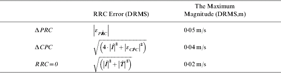
The summary of the maximum magnitude for the RRC error is shown in Table 1. The magnitude of estimated RRC is less than 0·02 m/s, and those of ΔCPC and ΔPRC, which are 0·04 m/s and 0·05 m/s, include too large an error to ignore. If the user compensated for the time latency of PRC, he would find a time latency error propagating into PRC. This can be expressed by δRRC⋅latency, and it depends on the extent of RRC error. The magnitude of RRC is now very small, and the error caused by setting RRC to zero results in the smallest amount developed within the three generation techniques. We therefore suggest setting RRC to zero in order to minimize the temporally decorrelated error.
Table 1. Summary of RRC error for each generation technique.
Static Test Result
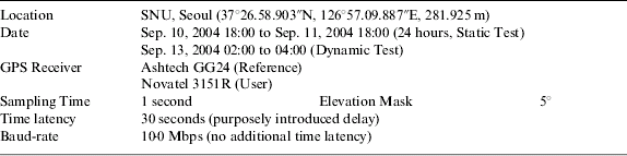
We organized an experiment test set, which proved our results. It comprises a reference station, a transmission method, and a user application. The TCP/IP server in the reference station broadcasts RTCM message version 2.1 without any modification. Two receivers in the user application are connected to the same computer and receive the correction message simultaneously via internet after a 30-second delay. According to the broadcast standard for the USCG DGPS, the PRC time-out limit is 30 seconds, so we cannot delay longer than this. The receiver used for the reference station is an Ashtech GG24 receiver, while the two for the user application are Novatel 3151R receivers. They are different from each other, but there is no problem because the RTCM message is a standard format. A splitter enables the same GPS signal to flow into both receivers. The only difference in this two-in-one system is that one uses the RRC to compensate for the 30-second latency, and the other does not. We did a zero-baseline static test for 24 hours to show the diurnal variation and the persistency of the position accuracy improvement without using RRC. We set the elevation angle mask at 5°. Full details are in Table 2.
Table 2. Summary of the static and dynamic test.
The zero-baseline static test result in 30-second latency is presented in Figure 6 and Table 3. From the horizontal DGPS results, we found that the RRC made the position noisy and caused it to jump far away from the origin. Moreover, the vertical result showed that the position compensated for by RRC had bias. If we use RRC at the future baud-rate (50 bps), a 95% horizontal position error is over 1 m and vertical error can be up to 3 m. On the other hand, setting RRC to zero can reduce these errors to 0·8 m and 1·5 m. This result therefore supports our previous suggestion that setting RRC to zero can help to reduce the temporally decorrelated error.

Figure 6. 24 hr horizontal (left) and vertical (right) positioning result.
Table 3. Position error (DRMS) of 24 hr processing.

3. SPATIALLY DECORRELATED ERROR
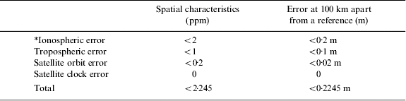
Errors that are spatially decorrelated depend on the geographic separation between the user and the site for which the corrections were computed. Local conditions within the ionosphere and the troposphere cause variable delays in the GPS ranging signals that distort the true range to the user. Table 4 shows the characteristics of spatially correlated GPS errors. The main drawback in lengthening the distance between the GPS RS and the DGPS user is the ionospheric error. In mid-latitude regions, this error cannot seriously affect the quality of GPS observations, unless there is ionospheric disturbance. Under normal conditions, ionospheric error in mid-latitude regions does not exceed a few parts per million. The range errors due to residual tropospheric and ephemeris error are a few centimetres if the length of the baseline is 100 km. When the length of the baseline is several kilometres, the effect of spatially correlated error is negligible. A length of several tens of kilometres, however, causes spatially correlated errors to have some influence upon the DGPS performance. Even though each measurement is corrected, residual ionospheric and tropospheric error can extend for several decimetres.
Table 4. The spatially decorrelated error property. (*Assuming that the GPS user is in the mid-latitude zone and not influenced by ionospheric scintillation.)

4. A GUIDELINE FOR ESTABLISHING DGPS RS REQUIREMENTS
We have examined the properties of temporally and spatially decorrelated errors independently. Using this approach, we can estimate the positioning error statistics at a specific baud-rate and at a distance from the reference station without taking measurements. The plot of these statistics shows how the baud-rate and coverage range influence the DGPS user's position accuracy.
Procedure to establish a Guideline
Firstly, a reference station should determine between the horizontal and vertical plane. Mariners are interested in horizontal rather than vertical accuracy. On the other hand, aviators on approach and landing have vertical accuracy requirements. The reference station should therefore relate to the main user's operational plane and requirements before a determination of the broadcasting baud-rate is made. Secondly, the average value of DOP and receiver noise of the PRC should be assessed. The noise statistics can be obtained from the elevation angle of the satellites and the receiver noise model. Thirdly, the spatially decorrelated error based on the geographic separation between the user and the reference station is required. The reference station should survey the dominant users' service distance or DGPS coverage to determine the range. The spatially decorrelated error, εPRC, S, is derived by using Table 4.
Fourthly, the temporally decorrelated error should be considered. Figure 7 shows the time-latency variation according to the transmission rate. We concluded that setting RRC to zero is the best way to reduce the temporally decorrelated error. Referring to Equation 25, this error (εPRC, T) can be expressed by Equation 27:
The fifth and final stage of this procedure is to calculate the user range error and position accuracy. A user range error (URE, σURE) can be expressed by the equation for the average value of DOP, the PRC error (![]() ), spatially (εPRC, S) and temporally (εPRC, T) decorrelated errors and receiver noise (σnoise). Assuming that there is no multi-path, we can expect to derive the accuracy by using the URE and DOP value. In the case of horizontal plane accuracy, we should use the HDOP for DOP. For the vertical plane, we should use VDOP.
), spatially (εPRC, S) and temporally (εPRC, T) decorrelated errors and receiver noise (σnoise). Assuming that there is no multi-path, we can expect to derive the accuracy by using the URE and DOP value. In the case of horizontal plane accuracy, we should use the HDOP for DOP. For the vertical plane, we should use VDOP.
Figure 8 provides a schematic approach to the complete procedure.

Figure 7. Minimum and maximum PRC latency of each baud-rate for nine satellites.

Figure 8. Block diagram of procedure to make a Guideline.
Examples of Using the Guideline
Let us take an example determination of the baud-rate for a DGPS server. Imagine that the reference station is established in the Seoul region at 37°26.58.903′′N. The reference station broadcasts RTCM messages for maritime users who are interested in horizontal accuracy. It follows the standard broadcast schedule of the US Coast Guard except for the Message Type 3. It broadcasts the Type 3 every minute not every 30 minutes, because it wants the user to start positioning as soon as the receiver is turned on. To minimize the temporally decorrelated error, RRC is set to zero. See Table 5 for a summary.
Table 5. Simulation summary.

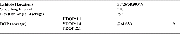
To get the average value of DOP and the receiver noise of the PRC, we logged the 24-hour data in a Trimble 4000ssi receiver. The average HDOP, VDOP, and elevation angle are shown in Table 6. The standard deviation of the receiver noise for 39° is 0·3 m, and that smoothed by a divergence-free Hatch filter is about 0·035 m.
Table 6. Average values in Seoul (37°N region).

If the available service range is 100 km, the spatially decorrelated error (εPRC, S) is 0·2245 m. The horizontal accuracy (2DRMS, 95%) varies with user receiver noise (0·3–1·0 m) and baud-rate (25–200 bps), as shown in Figure 9. The accuracy of the user 100 km away from the reference station (Figure 9, right) is slightly lower than zero-baseline accuracy (Figure 9, left) because of εPRC, S (0·2245 m).

Figure 9. Position accuracy degradation by spatially decorrelated error: Zero-base line accuracy (left) and 100 km apart user accuracy (right).
Let us take the DGPS target accuracy in the horizontal plane to be 1·5 m (95%). We need then to focus only upon the cyan colour line in Figure 10, which represents 1·5 m accuracy achieved by the user's receiver noise and baud-rate. If the standard deviation of most users' receiver noise is 0·5 m, the reference station can determine the rate at 36 bps. At this stage we should consider the integrity of the system. According to Brown (Reference Brown1994) in his NTIA report, the current integrity (time to alarm) is based upon the Type 9 message in the RTCM format and a data rate of 200 bps. The time to alarm of USCG is six seconds, and that of this report is 4·2 seconds. We should maintain not only the position accuracy, but also the response period of the alarm after reducing the baud-rate. Since the Type 9-3 message is set at 210 bits, it is impossible to reduce the rate below 50 bps with broadcasting a new correction message in 4·2 seconds. The reference station in this example should therefore broadcast the correction message at 50 bps.

Figure 10. Guide plot of position accuracy variation in user receiver noise and baud-rate. (For a reference station).
As another example, a user 100 km distant from the receiver in the previous scenario wants to purchase a receiver. The accuracy requirement is 3·5 m (95%) in a vertical plane, and the orange line in Figure 11 should be followed. This line meets 0·9 m of user receiver noise at 50 bps. Thus, the required receiver is the one whose noise standard deviation is 0·9 m.

Figure 11. Guide plot of position accuracy variation in user receiver noise and baud-rate. (For a user).
5. CONCLUSIONS
After being corrected by PRC, the user's position accuracy may still be degraded because the errors are decorrelated spatially and temporally. These errors can be understood independently, and this approach enables us to estimate the position accuracy of real DGPS users without measurements being needed.
The magnitude of PRC became small and more resistant to time latency after SA-off. To examine the temporally decorrelated error of PRC we studied the time rates of atmospheric delay and ephemeris error, and the noise characteristics of the pseudo-range and carrier phase. Through literature research, analysis of statistics, data from the IGS centre, accepted atmospheric models, and static test results, we came to the conclusion that the RRC is virtually zero. We can therefore minimize the temporally decorrelated error by setting RRC to zero. The error may be decorrelated by 2·245 m per 1000 km away from the reference station.
Taking the temporally and spatially decorrelated error into account, we suggest a guideline to determine the baud-rate and choose an appropriate receiver. Although a 30 or 40 bps rate enables the current position accuracy (1–3 m, 95%, horizontally) to be maintained, it is too low to broadcast an alarm message in six seconds. We therefore recommend that the US Coast Guard DGPS service broadcasts the correction message based on Type 9 at 50 bps. At this baud-rate, a user with noise whose standard deviation is 1 m can easily meet the USCG requirement. Furthermore, the duration of initial positioning is rapid, and the alarm message may be broadcast within six seconds.
In the post SA era, USCG redesigns the DGPS RS configuration are based on these results. We hope that this approach with its guidelines can be flexibly applied in the appropriate fields:
• determination of a reference station baud-rate to meet the required accuracy
• estimation of user accuracy at the current baud-rate
• finding the available range of the receiver noise and the reference station coverage
• choosing receivers suitable to accuracy requirements.
ACKNOWLEDGMENTS
The study was supported in part by a grant from the Brain Korea 21(BK-21) Programme for Mechanical and Aerospace Engineering Research at Seoul National University, and by John J. McMullen Associates (JJMA). We thank them for their valuable assistance. We are also grateful to the United States Coast Guard for their helpful suggestions and information.