2.1. Membrane geometry, kinematics and incompressibility

The lipid membrane is idealized as a two-dimensional manifold $\varOmega$ in three-dimensional space. Material points on $\varOmega$ are parametrized by a position field $\boldsymbol {r}(\theta ^\alpha ,t)$, where $\theta ^{\alpha }$ are surface coordinates and play a role analogous to that of a fixed coordinate system used to parametrize a control volume in the Eulerian description of classical fluid mechanics. Here and henceforth, Greek indices range over $\{1,2\}$ and, if repeated, are summed over that range. The local tangent basis on the surface is naturally obtained as $\boldsymbol {a}_{\alpha }=\boldsymbol {r}_{,\alpha }$ where commas identify partial derivatives with respect to $\theta ^{\alpha }$. The unit normal field is then given by $\smash {\boldsymbol {n}=\boldsymbol {a}_{1}\times \boldsymbol {a}_{2}/\vert \boldsymbol {a}_{1} \times \boldsymbol {a} _{2}\vert }$. The tangent basis also defines the surface metric $a_{\alpha \beta }=\boldsymbol {a}_{\alpha }\boldsymbol {\cdot } \boldsymbol {a}_{\beta }$ (or coefficients of the first fundamental form), a positive definite matrix, which is one of the two basic variables in surface theory. The other is the curvature $b_{\alpha \beta }$ (or coefficients of the second fundamental form) defined as $b_{\alpha \beta }= \boldsymbol {n}\boldsymbol {\cdot } \boldsymbol {r}_{,\alpha \beta }$. Of special interest are the mean $(\textrm{nm}^{-1})$ and Gaussian $(\textrm{nm}^{-2})$ curvatures, which will enter the Helfrich energy of the membrane and are defined, respectively, as

(2.1a,b)\begin{equation} H=\tfrac{1}{2}a^{\alpha \beta }b_{\alpha \beta},\quad K=\tfrac{1}{2}\varepsilon^{\alpha \beta}\varepsilon ^{\mu\eta }b_{\alpha \mu }b_{\beta \eta}. \end{equation}

Here, $a^{\alpha \beta }=(a_{\alpha \beta })^{-1}$ is the dual metric, and $\varepsilon ^{\alpha \beta }$ is the permutation tensor defined as $\varepsilon ^{12}=-\varepsilon ^{21}=1/\sqrt {a},$ $\varepsilon ^{11}=\varepsilon ^{22}=0$.

We assume that the surface $\varOmega$ is moving with time, and the velocity of a material point in the membrane is given by $\boldsymbol {u}(\theta ^\alpha ,t)=\dot {\boldsymbol {r}}=\partial \boldsymbol {{r}}/\partial t$. It can be expressed in components on the natural basis introduced above

(2.2)\begin{equation} \boldsymbol{u} = v^{\alpha }\boldsymbol{a}_{\alpha }+w\boldsymbol{n}, \end{equation}

where the components $v^\alpha$ capture the tangential lipid flow and $w$ is the normal surface velocity. The membrane is assumed to be incompressible, which prescribes a relationship between the in-plane velocity field and the curvature as (Arroyo & DeSimone Reference Arroyo and DeSimone2009; Rangamani et al. Reference Rangamani, Agrawal, Mandadapu, Oster and Steigmann2013)

(2.3)\begin{equation} v^\alpha_{;\alpha}=2Hw,\end{equation}

where the semi-colon refers to covariant differentiation with respect to the metric $a_{\alpha \beta }$.

2.2. Stress balance and equations of motion

We model the membrane as a thin elastic shell and, in the absence of inertia, the equations of motion are the equations of mechanical equilibrium. For a membrane subjected to a lateral pressure difference $p\,(\textrm{pN} \cdot \textrm{nm}^{-2})$ in the direction of the unit normal $\boldsymbol {n}$, these may be summarized as (Steigmann Reference Steigmann1999)

(2.4)\begin{equation} \boldsymbol{T}_{;\alpha }^{\alpha }+p\boldsymbol{n}=\boldsymbol{0},\end{equation}

where $\boldsymbol {T}^{\alpha }$ are the so-called stress vectors. The differential operation in (2.4) is the surface divergence

(2.5)\begin{equation} \boldsymbol{T}_{;\alpha }^{\alpha }=(\sqrt{a})^{-1}(\sqrt{a}\boldsymbol{T}^{\alpha })_{,\alpha }, \end{equation}

where $a=\det (a_{\alpha \beta })>0$. This framework encompasses all elastic surfaces for which the energy density responds to metric and curvature. For example, if the energy density per unit mass of the surface is $F(a_{\alpha \beta },b_{\alpha \beta }),$ then (Steigmann Reference Steigmann1999)

(2.6)\begin{equation} \boldsymbol{T}^{\alpha }=N^{\beta \alpha }\boldsymbol{a}_{\beta }+S^{\alpha }\boldsymbol{n}, \end{equation}

where

(2.7a,b)\begin{equation} N^{\beta \alpha }=\zeta^{\beta \alpha }+\pi^{\beta\alpha}+b_{\mu }^{\beta }M^{\mu \alpha}\quad \mathrm{and}\quad S^{\alpha }=-M_{;\beta }^{\alpha \beta}.\end{equation}

We have introduced the notation $\smash {b_{\beta }^{\alpha }=a^{\alpha \lambda }b_{\lambda \beta }}$. In (2.7a,b), $\smash {\zeta ^{\beta \alpha }}\ (\textrm{pN}\cdot\textrm{nm}^{-1})$ is the in-plane elastic stress tensor, $\smash {\pi ^{\beta \alpha }}\ (\textrm{pN}\cdot\textrm{nm}^{-1})$ is the intra-membrane viscous stress tensor due to surface flow and $M^{\alpha \beta }$ is the moment tensor due to curvature-induced elastic bending. We discuss constitutive equations for these various contributions in the next sections.

Substituting (2.6) and (2.7a,b) into (2.4), invoking the Gauss and Weingarten equations $\boldsymbol {a}_{\beta;\alpha }=b_{\beta \alpha } \boldsymbol {n}$ and $\boldsymbol {n}_{,\alpha }=-b_{\alpha }^{\beta }\boldsymbol {a} _{\beta }$ (Sokolnikoff Reference Sokolnikoff1951) and projecting the result onto the tangent and normal spaces of $\varOmega$ provides the three governing equations

(2.8a,b)\begin{equation} N_{;\alpha }^{\beta \alpha }-S^{\alpha }b_{\alpha }^{\beta }=0,\quad S_{;\alpha }^{\alpha }+N^{\beta \alpha }b_{\beta \alpha }+p=0, \end{equation}

which express stress balances in the tangential and normal directions.

2.3. Free energy of an elastic membrane with curvature-inducing proteins

The elastic contribution of the surface stress and the moment tensor are derived from a free energy and are expressed as (Steigmann Reference Steigmann1999)

(2.9a,b)\begin{equation} \zeta^{\beta \alpha}=\rho \left(\frac{\partial F}{\partial a_{\alpha \beta }}+ \frac{\partial F}{\partial a_{\beta \alpha }}\right),\quad M^{\alpha \beta}=\frac{\rho}{2} \left(\frac{\partial F}{\partial b_{\alpha \beta}}+ \frac{\partial F}{\partial b_{\beta \alpha}}\right).\end{equation}

Here, $F$ is the energy Lagrangian per unit mass defined as (Steigmann Reference Steigmann1999)

(2.10)\begin{equation} F(H,K,\rho)=\bar{F}(H,K)-\gamma/\rho, \end{equation}

where $\gamma$ is a Lagrange multiplier imposing the constraint of incompressibility, and $\rho$ is the membrane density which is assumed to be constant. It is customary to formulate the mechanics in terms of the free energy per unit area as (Steigmann et al. Reference Steigmann, Baesu, Rudd, Belak and McEleresh2003)

(2.11)\begin{equation} W=\rho \bar{F}. \end{equation}

For an elastic membrane with a density $\sigma\ (\textrm{nm}^{-2})$ of curvature-inducing proteins, we model this free energy $(\textrm{pN}\cdot\textrm{nm}^{-1})$ as the sum of elastic and chemical energies (Veksler & Gov Reference Veksler and Gov2007; Steigmann & Agrawal Reference Steigmann and Agrawal2011; Alimohamadi & Rangamani Reference Alimohamadi and Rangamani2018)

(2.12)\begin{equation} W(H,K,\sigma )=k[H-C(\sigma )]^{2}+\bar{k}K+k_BT\sigma\left[\log\left(\frac{\sigma}{\sigma_s}\right)-1\right]. \end{equation}

The first two terms correspond to the classical Helfrich free energy and involve the two bending moduli $k\ (\textrm{pN}\cdot \textrm{nm})$ and $\bar{k}\ (\textrm{pN}\cdot\textrm{nm})$. While these could in general depend on $\sigma$, we take them to be constant as is appropriate in the dilute limit. $C(\sigma)\ (\textrm{nm}^{-1})$ is the protein-induced spontaneous curvature and is assumed to depend linearly on protein density (Veksler & Gov Reference Veksler and Gov2007; Steigmann & Agrawal Reference Steigmann and Agrawal2011; Gov Reference Gov2018)

(2.13)\begin{equation} C=\ell\sigma, \end{equation}

where the constant $\ell\ (\textrm{nm})$ is a characteristic length scale associated with the embedded protein. The last term in (2.12) is the entropic contribution due to thermal diffusion of proteins (Gov Reference Gov2018), where $k_BT\ (\textrm{pN}\cdot\textrm{nm})$ is the thermal energy and $\sigma _s\ (\textrm{nm}^{-2})$ denotes the saturation density of proteins on the membrane.

Inserting (2.12) for the free energy into (2.9a,b) provides expressions for the elastic stress and moment tensors as

(2.14)\begin{gather} \zeta^{\alpha\beta}=-2k(H-\ell \sigma) b^{\alpha \beta}-2\bar{k}Ka^{\alpha \beta}-\gamma a^{\alpha \beta}, \end{gather}

(2.15)\begin{gather}M^{\alpha\beta}=k(H-\ell \sigma) a^{\alpha\beta}+\bar{k}(2Ha^{\alpha\beta}-b^{\alpha\beta}). \end{gather}

2.4. Viscous stress

In the presence of surface flow, a viscous stress also develops in the membrane. The deviatoric part of the viscous stress tensor $\pi ^{\alpha \beta }$ is assumed to depend linearly on strain rate as (Scriven Reference Scriven1960)

(2.16)\begin{equation} \pi^{\alpha \beta}=\nu a^{\alpha \mu}a^{\beta \eta}\dot{a}_{\mu \eta}, \end{equation}

where $\nu$, a positive constant, is the intra-membrane surface viscosity. Further expanding this expression, we obtain

(2.17)\begin{equation} \pi^{\alpha \beta }=2\nu [a^{\alpha \mu }a^{\beta \eta }d_{\mu\eta}-wb^{\alpha \beta }], \end{equation}

where $d_{\mu \eta }=(v_{\mu;\eta }+v_{\eta;\mu })/2$ is the surface rate-of-strain tensor.

2.5. Conservation equation for protein transport

To complete the model, we specify a transport equation for the protein density $\sigma$. Mass conservation can be expressed as

(2.18)\begin{equation} \frac{\partial \sigma}{\partial t} +m^{\alpha}_{;\alpha}=0, \end{equation}

where $m^\alpha$ denotes the protein flux. This flux has contributions from advection by the surface flow as well as from gradients in chemical potential. Following Steigmann & Agrawal (Reference Steigmann and Agrawal2011), it can be derived from first principles as

(2.19)\begin{equation} m^\alpha=\left[v^\alpha -\frac{1}{f}a^{\alpha\beta}W_{\sigma,\beta}\right]\sigma, \end{equation}

where $f\ (\textrm{pN}\cdot\textrm{s}\cdot\textrm{nm}^{-1})$ is the hydrodynamic drag coefficient of a protein and $W_\sigma =\partial W/\partial \sigma$.

2.6. Summary of the governing equations

We summarize the governing equations for the membrane and protein dynamics. The tangential momentum balance, obtained by inserting (2.14), (2.15) and (2.17) for the stresses into equation (2.8a), is expressed as

(2.20)\begin{align} \lambda _{,\alpha }-4\nu wH_{,\alpha }+2\nu (a^{\beta\mu }d_{\alpha \mu;\beta }-w_{,\beta }b_{\alpha }^{\beta })= -\sigma_{,\alpha} \left[k_BT\log\left(\frac{\sigma}{\sigma_s}\right) -2k \ell (H-\ell \sigma)\right],\end{align}

where we have introduced the membrane tension $(\textrm{pN}\cdot\textrm{nm}^{-1})\ \lambda =-(W+\gamma )$. Along with the surface incompressibility condition

(2.21)\begin{equation} v_{;\alpha }^{\alpha}-2wH=0, \end{equation}

(2.20) constitutes the governing equation for the intra-membrane flow. We note the similarity with the Stokes equations, where the tension $\lambda$ plays a role analogous to the pressure in classical incompressible flow (Bahmani et al. Reference Bahmani, Christenson and Rangamani2016). The right-hand side captures the forcing by the protein distribution on the flow. Similarly, the normal force balance (2.8b) provides the so-called shape equation, written after simplification as

(2.22)\begin{align} & k{\rm \Delta} (H-\ell\sigma)+2k(H-\ell\sigma)(2H^{2}-K) -2H\left[k_BT\sigma\left(\log\left(\frac{\sigma}{\sigma_s}\right)-1\right)+k(H-\ell\sigma)^{2}\right] \nonumber\\ &\quad -2\nu [ b^{\alpha \beta }d_{\alpha \beta } -w(4H^{2}-2K)] =p+2\lambda H, \end{align}

where ${\rm \Delta} (\cdot )=(\cdot )_{;\alpha \beta }a^{\alpha \beta }$ is the surface Laplacian. Equation (2.22) can be interpreted as the governing equation for the position field $\boldsymbol {r}$. Finally, the model is completed by the advection–diffusion equation for the protein density, which is written

(2.23)\begin{equation} \frac{\partial \sigma}{\partial t}+ (v^{\alpha} \sigma)_{;\alpha} = Da^{\alpha \beta} \sigma_{,\alpha \beta}-\frac{2k \ell }{f}[a^{\alpha \beta}(H-\ell \sigma)_{,\alpha} \sigma_{,\beta}+\sigma a^{\alpha \beta}(H-\ell \sigma)_{,\alpha \beta}]. \end{equation}

The first term on the right-hand side captures Fickian diffusion of proteins, with diffusivity $D\ (\textrm{nm}^2\cdot\textrm{s}^{-1})$ given by the Stokes–Einstein relation: $D=k_B T/f$. The second term captures the interaction of the curvature and protein gradients. The third term captures the effect of membrane shape on protein transport: mismatch between the mean curvature and the protein-induced spontaneous curvature serves as a source term for the transport of protein on the membrane surface.

2.7. Comparison with other existing models

The equations of motion (2.8) have appeared in the literature in many different forms. For example, the tangential stress balance (2.8a) is similar to (9) of Salbreux & Jülicher (Reference Salbreux and Jülicher2017) and (1) of Mietke, Julicher & Sbalzarini (Reference Mietke, Julicher and Sbalzarini2019). We eventually obtain (2.20) from this equation by using the constitutive relation (2.17) for the viscous stress, an equivalent expression of which can be found in (D11) of Torres-Sanchez et al. (Reference Torres-Sanchez, Millan and Arroyo2019). The final form of the tangential balance (2.20) also correlates to their equation (D9). Similarly, the normal force balance relation (2.8b) compares with (10) of Salbreux & Jülicher (Reference Salbreux and Jülicher2017) and (2) of Mietke et al. (Reference Mietke, Julicher and Sbalzarini2019). The final form of the force balance relations (2.20)–(2.22) captures the effect of curvature-inducing proteins that diffuse in the plane of the membrane. This differs from the model of Mietke et al. (Reference Mietke, Julicher and Sbalzarini2019) where the effect of protein-induced active tension was considered, or from the model of Salbreux & Jülicher (Reference Salbreux and Jülicher2017), which includes a contribution from the external stress and torque applied by the extracellular matrix. The advection–diffusion equation (2.23) in our model is also similar to (13) of Mietke et al. (Reference Mietke, Julicher and Sbalzarini2019), (3.27) of Mikucki & Zhou (Reference Mikucki and Zhou2017), (2.12) of Nitschke, Voigt & Wensch (Reference Nitschke, Voigt and Wensch2012) and (4) of Gera & Salac (Reference Gera and Salac2017). These studies, however, did not include the strong coupling between bending and diffusion in (2.23), which results from the curvature inducing property of the membrane proteins. In the model presented by Mietke et al. (Reference Mietke, Julicher and Sbalzarini2019), the coupling between bending and diffusion occurs through an active tension induced by the proteins. Mikucki & Zhou (Reference Mikucki and Zhou2017) calculated the phase field of protein density in an inviscid framework, Nitschke et al. (Reference Nitschke, Voigt and Wensch2012) solved the coupled in place flow and higher-order diffusion equation on a convective surface, while Gera & Salac (Reference Gera and Salac2017) solved a Cahn–Hilliard equation on a pre-existing curved surface.

3.1. Linearization and dimensional analysis

In this section, we specialize the governing equations presented in § 2.6 in a Monge parametrization assuming small deflections from the flat plane.

3.1.1. Governing equations in the linear deformation regime

The surface parametrization for a Monge patch is given by

(3.1)\begin{equation} \boldsymbol{r}(x,y,t)=x\boldsymbol{i}+y\boldsymbol{j}+z(x,y,t)\boldsymbol{k}, \end{equation}

where unit vectors $(\boldsymbol {i},\boldsymbol {j},\boldsymbol {k})$ form a fixed Cartesian orthonormal basis, and $z(x,y,t)$ is the deflection from the $(x,y)$ plane. The tangent and normal vectors are given by

(3.2a–c)\begin{equation} \boldsymbol{a}_1=\boldsymbol{i}+z_{,x}\boldsymbol{k},\quad \boldsymbol{a}_2=\boldsymbol{j}+z_{,y}\boldsymbol{k},\quad \boldsymbol{n}=\frac{1}{(1+z_{,x}^2+z_{,y}^2)^{1/2}}(-z_{,x} \boldsymbol{i}-z_{,y} \boldsymbol{j}+\boldsymbol{k}). \end{equation}

The surface metric ($a_{\alpha \beta }$) and curvature metric ($b_{\alpha \beta }$) take the following forms

(3.3a,b)\begin{equation} a_{\alpha \beta}= \begin{bmatrix} 1+z_{,x}^2 & z_{,x} z_{,y} \\ z_{,y} z_{,x} & 1+z_{,y}^2 \end{bmatrix},\quad b_{\alpha \beta}=\frac{1}{(1+z_{,x}^2+z_{,y}^2)^{1/2}} \begin{bmatrix} z_{,xx} & z_{,xy} \\ z_{,yx} & z_{,yy} \end{bmatrix}. \end{equation}

We further assume that deflections of the membrane from the flat configuration are small and simplify the governing equations in the limit of weak surface gradients $|\boldsymbol {\nabla } z|\ll 1$ by neglecting quadratic terms in $|\boldsymbol {\nabla } z|$ (Do Reference Do1976). In this limit, differential operators in the space of the membrane reduce to the Cartesian gradient, divergence and Laplacian in the $(x,y)$ plane. The linearized governing equations for the intra-membrane flow become

(3.4)\begin{equation} \boldsymbol{\nabla}\boldsymbol{\cdot}\boldsymbol{v}=2wH, \\[-1pc]\nonumber\end{equation}

(3.5)\begin{align} & \boldsymbol{\nabla} \lambda +\nu {\nabla}^2 \boldsymbol{v}+\nu \boldsymbol{\nabla}(\boldsymbol{\nabla}\boldsymbol{\cdot}\boldsymbol{v})-4\nu w \boldsymbol{\nabla} H-2\nu \boldsymbol{\nabla} w \boldsymbol{:} \boldsymbol{\nabla}\boldsymbol{\nabla}z \nonumber\\ &\quad =k \left({\nabla}^2 z-2\ell \sigma \right) \ell \boldsymbol{\nabla} \sigma - k_BT\log\left(\frac{\sigma}{\sigma_s}\right)\boldsymbol{\nabla} \sigma, \end{align}

whereas the shape equation expressing the normal momentum balance is

(3.6)\begin{align} & k\left(\frac{1}{2} {\nabla}^4 z -\ell {\nabla}^2 \sigma \right)-{\nabla}^2 z \left[k_BT\sigma\left(\log\left(\frac{\sigma}{\sigma_s}\right)-1\right)+k \ell^2 \sigma^2\right] \nonumber\\ &\quad -\nu \left(\boldsymbol{\nabla} {\boldsymbol{v}}+ \boldsymbol{\nabla}\boldsymbol{v}^{\textrm{T}}\right)\boldsymbol{:} \boldsymbol{\nabla} \boldsymbol{\nabla}z=p+\lambda{\nabla}^2 z. \end{align}

The transport equation for the protein density simplifies to

(3.7)\begin{equation} \frac{\partial {\sigma}}{\partial t}+ \boldsymbol{\nabla}\boldsymbol{\cdot}(\sigma \boldsymbol{v})=D{\nabla}^2 \sigma-\frac{k\ell }{f} \boldsymbol{\nabla} \left({\nabla}^2 z -2\ell \sigma \right)\boldsymbol{\cdot} \boldsymbol{\nabla} \sigma-\frac{k\ell \sigma}{f} \left( {\nabla}^4 z -2\ell {\nabla}^2 \sigma \right). \end{equation}

We also note the linearized kinematic relation for the normal velocity

(3.8)\begin{equation} w=\frac{\partial z}{\partial t}. \end{equation}

3.1.2. Non-dimensionalization

We scale this system of equations using the following reference values. Length is non-dimensionalized by the size $L$ of the domain, protein density by its reference value $\sigma _0$ and membrane tension by its far-field value $\lambda _0$. We also use the characteristic velocity scale $v_c=\lambda _0 L/\nu$ and time scale $t_c= L^2/D$. Denoting dimensionless variables with a tilde, the scaled governing equations are

(3.9)\begin{equation} \tilde{\boldsymbol{\nabla}}\boldsymbol{\cdot}\tilde{\boldsymbol{v}}=2\tilde{w} \tilde{H}, \end{equation}

(3.10)\begin{align} & \tilde{\boldsymbol{\nabla}} \tilde{\lambda} +\tilde{\nabla}^2 \tilde{\boldsymbol{v}}+ \tilde{\boldsymbol{\nabla}} (\tilde{\boldsymbol{\nabla}}\boldsymbol{\cdot} \tilde{\boldsymbol{v}})-4\tilde{w}\tilde{\boldsymbol{\nabla}} \tilde{H}-2\tilde{\boldsymbol{\nabla}}\tilde{w}\boldsymbol{:}\tilde{\boldsymbol{\nabla}}\tilde{\boldsymbol{\nabla}}\tilde{z} \nonumber\\ &\quad =\tilde{\boldsymbol{\nabla}} \tilde{\sigma} \left[\frac{{\vphantom{A}\smash{2 \hat{C} \hat{B}}}}{\hat{T}} \tilde{\nabla}^2 \tilde{z} -\frac{4 \hat{C}^2 \hat{B}^2}{\hat{T}}\tilde{\sigma} -\frac{2\hat{C}}{\hat{T}} \log\left(\frac{\tilde{\sigma}}{\tilde{\sigma}_s} \right)\right], \end{align}

(3.11)\begin{align} & \tilde{\nabla}^4\tilde{z}-{\vphantom{A}\smash{2 \hat{C} \hat{B}}} \tilde{\nabla}^2 \tilde{\sigma} - \hat{C} \tilde{\nabla}^2 \tilde{z}\left[2\tilde{\sigma}\left(\log \left(\frac{\tilde{\sigma}}{\tilde{\sigma}_s}\right)-1 \right)+2 \hat{C} \hat{B}^2 \tilde{\sigma}^2\right] \nonumber\\ &\quad -\hat{T} (\tilde{\boldsymbol{\nabla}} \tilde{\boldsymbol{v}}+\tilde{\boldsymbol{\nabla}} \tilde{\boldsymbol{v}}^{\textrm{T}})\boldsymbol{:}\tilde{\boldsymbol{\nabla}} \tilde{\boldsymbol{\nabla}}\tilde{z} = \hat{P}+\hat{T} \tilde{\lambda}\tilde{\nabla}^2 \tilde{z}, \end{align}

(3.12)\begin{align} & \smash{\frac{\partial \tilde{\sigma}}{\partial \tilde{t}}}+{{Pe}} \left(\tilde{\boldsymbol{v}}\boldsymbol{\cdot} \tilde{\boldsymbol{\nabla}} \tilde{\sigma}+\tilde{\sigma}\tilde{\boldsymbol{\nabla}}\boldsymbol{\cdot}\tilde{\boldsymbol{v}}\right)= \left(1+2 \hat{C} \hat{B}^2\tilde{\sigma}\right)\tilde{\nabla}^2 \tilde{\sigma} \nonumber\\ &\quad +2\hat{C} \hat{B}^2 |\tilde{\boldsymbol{\nabla}}\tilde{\sigma}|^2-\hat{B}\left(\tilde{\sigma} \tilde{\nabla}^4\tilde{z}+\tilde{\boldsymbol{\nabla}}\tilde{\nabla}^2\tilde{z}\boldsymbol{\cdot} \tilde{\boldsymbol{\nabla}} \tilde{\sigma}\right). \end{align}

The expression for the normal velocity also becomes:

(3.13)\begin{equation} \tilde{w}=\frac{1}{{{Pe}}}\frac{\partial \tilde{z}}{\partial \tilde{t}}. \end{equation}

The dynamics is governed by five dimensionless parameters defined as follows. The ratio of the chemical potential to the bending rigidity of the membrane is denoted by $\hat {C}={L^2 k_B T\sigma _0}/{k}$. The ratio of the length scale induced by the proteins and the membrane domain is given by $\hat {L}=\ell L \sigma _0$. The ratio of the intrinsic length scale of the membrane to the domain size is given by $\hat {T}={2L^2 \lambda _0}/{k}$. The ratio between the bulk pressure and bending rigidity is denoted by $\hat {P}={2L^3p}/{k}$. Finally, the Péclet number $Pe={\lambda _0 L^2}/{\nu D}$ compares the advective transport rate to the diffusive transport rate. We define $\hat {B}=\hat {L}/\hat {C}$ for convenience of simulations and cast the equations in terms of $\hat {L}$, $\hat {B}$, $\hat {T}$ and $Pe$. Further, we assume that there is no pressure difference across the membrane ($\hat {P}=0$).

3.2. One-dimensional simulations

We first explore the interplay between membrane bending and protein diffusion in the special case of a membrane that deforms as a string in one dimension, with a shape parameterized as $\tilde {z}(\tilde {x},\tilde {t})$. The flow of lipids does not play a role in this scenario, and as a result in-plane velocity-dependent terms vanish in (3.9)–(3.12). The system of governing equations reduces to

(3.14)\begin{gather} \frac{\partial \tilde{\lambda}}{\partial \tilde{x}}= \frac{\partial \tilde{\sigma} }{\partial \tilde{x}} \left[\frac{{\vphantom{A}\smash{2 \hat{C} \hat{B}}}}{\hat{T}} \frac{\partial^2 \tilde{z}}{\partial \tilde{x}^2} -\frac{4 \hat{C}^2 \hat{B}^2} {\hat{T}} \tilde{\sigma} -\frac{2 \hat{C}}{\hat{T}}\log \left(\frac{\tilde{\sigma}}{\tilde{\sigma}_s}\right)\right], \end{gather}

(3.15)\begin{gather}\frac{\partial \tilde{\sigma}}{\partial \tilde{t}} = (1+2 \hat{C} \hat{B}^2 \tilde{\sigma}) \frac{\partial^2\tilde{\sigma}}{{\partial {\tilde{x} }}^2 } + 2 \hat{C} \hat{B}^2 \left(\frac{\partial \tilde{\sigma}}{\partial \tilde{x}}\right)^2-\hat{B}\left[\tilde{\sigma} \frac{\partial^4 \tilde{z}}{{\partial {\tilde{x} }}^4 }+\frac{\partial \tilde{\sigma}}{\partial \tilde{x}} \frac{\partial }{\partial \tilde{x}}\left( \frac{\partial^2 \tilde{z}}{\partial \tilde{x}^2} \right)\right], \end{gather}

(3.16)\begin{gather}\frac{\partial^4 \tilde{z}}{{\partial {\tilde{x} }} ^4}-{\vphantom{A}\smash{2 \hat{C} \hat{B}}} \frac{\partial^2 \tilde{\sigma}}{{\partial {\tilde{x} }} ^2} - \hat{C} \frac{\partial^2\tilde{z}}{{\partial {\tilde{x} }} ^2}\left[2\tilde{\sigma}\left(\log \left(\frac{\tilde{\sigma}}{\tilde{\sigma}_s}\right)-1 \right)+2 \hat{C} \hat{B}^2 \tilde{\sigma}^2\right] =\hat{P}+\hat{T} \tilde{\lambda} \frac{\partial^2 \tilde{z}}{{\partial {\tilde{x} }}^2}. \end{gather}

Equations (3.14)–(3.16) are solved numerically using a finite-difference scheme coded in Fortran 90 (numerical codes are available at https://github.com/armahapa/transport\_phenomena\_in\_membranes). The tangential momentum balance (3.14), which can be viewed as an equation for the tension $\tilde {\lambda }$, is solved subject to the condition $\tilde {\lambda }(\tilde {x}=0.5)=1$, whereas the shape equation (3.16) is solved subject to clamped boundary conditions $\tilde {z}=0$ and $\partial \tilde {z}/\partial \tilde {x}=0$ at both ends of the domain $\tilde {x}=-0.5,0.5$.

We first analysed the evolution of a symmetric patch of protein defined as $\tilde {\sigma }(\tilde {x},\tilde {t}=0)=1/2[\tanh (20(\tilde {x}+0.1))-\tanh (20 (\tilde {x}-0.1))]$, subject to no-flux boundary conditions on $\tilde {\sigma }$ at the ends of the domain. Results from these simulations are shown in figure 1. In response to this protein distribution, the initial configuration of the membrane is bent (see figure 1(a) at $t=0$). Over time, $\tilde {\sigma }$ homogenizes as a result of diffusion, and therefore the deflection $\tilde {z}$ decreases. At steady state, the distribution of protein is uniform on the membrane and $\tilde {z}$ is everywhere zero. The time evolution of $\tilde {z}$ at the centre of the string, corresponding to the maximum deflection, is shown in figure 1(b).

Figure 1. Protein density and membrane deformation in one dimension as functions of time, when an initial protein distribution and no-flux boundary conditions are prescribed. (a) Distribution of protein density plotted on the deformed one-dimensional membrane. (b) Time evolution of the maximum membrane deflection $\tilde {z}_c(\tilde {t})=\tilde {z}(1/2,\tilde {t})$.

As a second example, we discuss the case where the protein density is initially zero and a time-dependent protein flux is prescribed at both boundaries as shown in figure 2(a). In response to the influx at the boundaries, the membrane deforms out of plane as the protein density increases; see figure 2(b). Once the flux returns to zero, diffusion homogenizes the protein, and the membrane height begins to decrease again. This effect is observed clearly by looking at the deformation at the centre of the string as a function of time in figure 2(c), which closely follows the dynamics of the boundary flux shown in figure 2(a).

Figure 2. Evolution of membrane deformation and protein distribution when an influx of protein is prescribed at both boundaries. (a) Dimensionless boundary protein flux as a function of time. (b) Distribution of protein density plotted on the deformed membrane for $\smash {\hat {C}}=2.48\times 10^{-1}$. Each shape corresponds to a specific time point. (c) Time evolution of the maximum membrane deflection $\tilde {z}_c$ for $\smash {\hat {C}}=2.48\times 10^{-1}$. Symbols in panels (a,c) correspond to the time traces shown in (b).

In both examples of figures 1 and 2, we note that the protein distribution becomes uniform at long times (in the absence of any boundary flux), and as a result the membrane returns to its flat reference shape. At first glance, this result seems counter-intuitive since there is a non-zero density of curvature-inducing proteins on the membrane. But as Chabanon and Rangamani showed previously, for a uniform distribution of proteins with no-flux boundary conditions on the membranes, minimal surfaces are admissible solutions for the membrane geometry (Chabanon & Rangamani Reference Chabanon and Rangamani2018, Reference Chabanon and Rangamani2019). In the case of closed geometries on vesicle, constant mean curvature surfaces are admissible solutions (Zhong-Can & Helfrich Reference Zhong-Can and Helfrich1989; Seifert Reference Seifert1993; Góźdź & Gompper Reference Góźdź and Gompper1998; Campelo & Hernández-Machado Reference Campelo and Hernández-Machado2007). In the case of interest here, a flat membrane is the admissible solution for the boundary conditions associated with $\tilde {z}$, and a proof of this result is given in appendix A.

3.3. Two-dimensional simulations

3.3.1. Numerical implementation

We solved the set of governing equations (3.9)–(3.12) in two dimensions inside a square domain using a finite-difference technique that we outline here. Our numerical scheme is second order in space and first order in time. We note that time only appears explicitly in the advection–diffusion equation (3.12) for the protein density: we solve it using a semi-implicit scheme wherein the linear diffusion term is treated implicitly while the nonlinear advective terms and curvature-induced transport terms are treated explicitly. The remaining governing equations are all elliptic in nature and can be recast as a series of Poisson problems as we explain. First, we note that the shape equation (3.11) is biharmonic and can thus be recast into two nested Poisson problems providing the shape $\tilde {z}$ at a particular time step. To solve for the surface tension $\tilde {\lambda }$, we take the divergence of the tangential momentum balance (3.10) and combine it with the continuity equation (3.9) to obtain the Poisson equation

(3.17)\begin{equation} \tilde{\nabla}^2\tilde{\lambda}+f=0, \end{equation}

where

(3.18)\begin{align} f &= 4\tilde{H}\tilde{\nabla}^2\tilde{w}-2\tilde{\boldsymbol{\nabla}}\tilde{\boldsymbol{\nabla}}\tilde{z}\boldsymbol{:} \tilde{\boldsymbol{\nabla}}\tilde{\boldsymbol{\nabla}} \tilde{w}\nonumber\\ &\quad -\frac{{\vphantom{A}\smash{2 \hat{C} \hat{B}}}}{\hat{T}}\tilde{\boldsymbol{\nabla}} \tilde{\nabla}^2 \tilde{z}\boldsymbol{\cdot} \tilde{\boldsymbol{\nabla}} \tilde{\sigma}-\left[\frac{{\vphantom{A}\smash{2 \hat{C} \hat{B}}}}{\hat{T}} \tilde{\nabla}^2 \tilde{z}- \frac{2\hat{C}}{\hat{T}}\log \left(\frac{\tilde{\sigma}}{\tilde{\sigma}_s} \right)\right]\tilde{\nabla}^2 \tilde{\sigma} \nonumber\\ &\quad +\frac{2\hat{C}}{\hat{T}}\tilde{\boldsymbol{\nabla}} (\log\tilde{\sigma}) \boldsymbol{\cdot} \tilde{\boldsymbol{\nabla}} \tilde{\sigma} +\frac{2 \hat{C}^2 \hat{B}^2}{\hat{T}} \tilde{\nabla}^2 \tilde{\sigma}^2. \end{align}

Note that there is no natural boundary condition on $\tilde {\lambda }$ at the edges of the domain. To approximate an infinite membrane, we first estimate the tension along the four edges using the integral representation

(3.19)\begin{equation} \tilde{\lambda}(\tilde{\boldsymbol{r}})=1+\int_{\varOmega}G(\tilde{\boldsymbol{r}}- \tilde{\boldsymbol{r}}_0)f(\tilde{\boldsymbol{r}}_0)\,\mathrm{d}A(\tilde{\boldsymbol{r}}_0), \end{equation}

where $G(\boldsymbol {r})=-\log r/2{\rm \pi}$ is the two-dimensional (2-D) Green's function for Poisson's equation in an infinite domain. The calculated tension along the edges is then used as the boundary condition for (3.17), where the normal velocity component at the current time step $k$ is calculated as

(3.20)\begin{equation} \tilde{w}^k=\frac{1}{{{Pe}}}\frac{\tilde{z}^k-\tilde{z}^{k-1}}{{\rm \Delta}\tilde{t}}. \end{equation}

With knowledge of the membrane tension, the tangential momentum balance (3.10) then provides two modified Poisson problems for the in-plane velocity components. Note that the equations for $\tilde {z}$, $\tilde {\lambda }$ and $\tilde {\boldsymbol {v}}$ are nonlinearly coupled through the various forcing terms in their respective Poisson problems. To remedy this problem, we iterate their solution until every variable converges with a tolerance limit of $5\times 10^{-7}$ before proceeding to the next time step. All the results presented below were obtained on a spatial uniform grid of size $201\times 201$ and with a dimensionless time step of ${\rm \Delta} \tilde {t}=10^{-4}$. We used Fortran 90 for compiling and running the algorithm. As we show in appendix B, the numerical method was successfully validated by comparison with a Stokes–Neumann formulation (Glowinski et al. Reference Glowinski, Pan, Juarez, Dean, Capasso and Périaux2005).

3.3.2. Two-dimensional simulation results

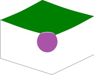
Using the numerical scheme described above, we solved the linearized two-dimensional governing equations (3.9)–(3.12) for different initial conditions. In all cases, the boundary conditions for the membrane shape were set to $\tilde {z}=0$ and $\boldsymbol {\nu }\boldsymbol {\cdot }\boldsymbol {\nabla } \tilde {z} =0$ where $\boldsymbol {\nu }$ is the in-plane normal to the edge of the domain, and no-flux boundary conditions were enforced on the protein distribution. We considered three different initial conditions for the protein density as depicted in figure 3, namely: a single circular patch at the centre of the domain (figure 3a), two identical patches placed at diametrically opposite ends of the domain (figure 3b) and four patches centred in each quadrant of the domain (figure 3c). The total mass of protein is the same in all three cases, only the initial spatial distribution is different. For the velocity and tension, we maintain open boundary conditions as noted in § 3.3.1.

Figure 3. System set-up and initial condition used in 2-D simulations. All 2-D simulations are performed for a linearized Monge patch. We simulate the dynamics for three different initial distributions of proteins as shown. The total area fraction of protein is same for the three cases, with proteins covering 10 % of the total area. (a) Single patch of protein placed at the centre $(0,0)$. (b) Two patches of protein placed at diametrically opposite positions with centre locations $(-0.25,-0.25)$ and $(0.25,0.25)$. (c) Four patches of proteins placed at four diagonal positions: $(-0.25,-0.25)$, $(-0.25, 0.25)$, $(0.25,-0.25)$ and $(0.25,0.25)$. The following abbreviations are used in subsequent figures to track the system behaviour: COM: centre of the membrane, COP: centre of the patch, CRM: corner of the membrane and PFM: protein-free membrane.

We tracked the dynamics of the membrane shape, protein distribution, membrane tension and velocity for a single patch of proteins corresponding to figure 3(a) in figure 4. The initial membrane configuration is bent to accommodate the initial distribution of proteins (figure 4a), and the membrane tension for this initial distribution is heterogeneous as seen in figure 4(d), consistent with our previous results (Rangamani et al. Reference Rangamani, Mandadapu and Oster2014; Hassinger et al. Reference Hassinger, Oster, Drubin and Rangamani2017). Over time, the proteins diffuse from the centre of the patch across the membrane, tending towards a homogeneous distribution (figure 4b,c), and this process is accompanied by a reduction in the membrane deflection. The homogenization of proteins results in homogenization of the membrane tension, which approaches its value at infinity (figure 4e,f). The tangential velocity is directed outward (figure 4g–i), and the dimensionless magnitude of the maximum velocity in figure 4(g) is $4.8 \times 10^{-3}$. Expectedly, the magnitude of this velocity decreases with time as seen in figure 4(h,i).

Figure 4. Dynamics of the evolution of membrane shape, protein distribution, membrane tension and tangential velocity field for a single patch of protein at three different times. (a–c) Distributions of membrane protein density are shown at dimensionless times $1\times 10^{-3}$, $5\times 10^{-3}$ and $2.5\times 10^{-2}$. (d,e) Distributions of membrane tension at the same non-dimensional times. (g–i) Tangential velocity fields shown at the same non-dimensional times. Arrows are scaled according to tangential velocity magnitude, with a maximum dimensionless velocity of $4.3\times 10^{-3}$.

When the proteins are distributed in two and four patches as shown in figure 3(b,c), we found that the overall behaviour of the system was quite similar to a single patch with some changes to the dynamics. First, because each patch had a lower density of proteins (half or quarter), the initial deformation was smaller and the protein distribution homogenized faster than in the case of a single patch (figure 5a,b). Similarly, the typical magnitude of membrane tension variations (figure 5c,d) and of the tangential velocity field (figure 5e,f) was also smaller to begin with and the system attained the homogeneous distribution rapidly.

Figure 5. Dynamics of the evolution of membrane shape, protein distribution, membrane tension and tangential velocity field for two and four patches of protein at dimensionless time $\tilde {t}=5 \times 10^{-3}$. The left column shows the distribution of protein density (a), membrane tension (c) and tangential velocity (e) for two patches of protein. The right column shows the distribution of protein density (b), membrane tension (d) and tangential velocity (f) for four patches of protein. The magnitude of the maximum dimensionless tangential velocity is $1.6\times 10^{-2}$ in the case of two patches, and $4.1\times 10^{-3}$ in the case of four patches.

To compare the effects of one, two and four patches directly, we plotted the membrane deformation (figure 6), membrane protein distribution (figure 7) and membrane tension distribution (figure 8) at different locations for each case. The initial deformation is different for the different cases because of the differences in the local density of proteins. For a single patch, we observed that the maximum deformation occurs at the centre of the patch and it takes a longer time for this deformation to go to zero in the case of a single patch compared to multiple patches (compare figure 6a to 6b,c). In the case of two and four patches, we also observe a small positive deformation at the centre of the membrane and in the protein-free membrane. This can be explained by the fact that the continuity conditions of the surface will result in a small but upward displacement in protein-free regions in response to the large downward displacement in the regions where the proteins are initially present.

Figure 6. Temporal evolution of the membrane deflection at the various locations defined in figure 3 for a single patch of protein (a), two patches (b) and four patches (c).

Figure 7. Temporal evolution of the protein density at the locations defined in figure 3 for a single patch of protein (a), two patches (b) and four patches (c).

Figure 8. Temporal evolution of the membrane tension at the locations defined in figure 3 for a single patch of protein (a), two patches (b) and four patches (c).

Comparing the protein dynamics for one, two and four patches, we observed that increasing the number of patches decreases the time it takes for the protein distribution to homogenize across the membrane domain (figure 7). Thus, although membrane bending and protein distribution are coupled, the distribution of multiple patches weakens the coupling and promotes rapid homogenization of the membrane proteins. While the steady state protein distribution is the same in all cases, the dynamics with which the protein-free regions show an appreciable increase in proteins also depends on the initial distribution of proteins. For example, in the case of a single patch, CRM takes much longer to reach steady state compared to the case of two or four patches. Figure 7 shows that for the initial conditions of a single patch and of four patches of protein, $\tilde {\sigma }$ approaches the uniform protein density monotonically. But for the case of two patches, the time evolution of the protein density is not monotonic, and we found the density of protein at the corner of the membrane exceeds the density at the COP for a brief time interval. We investigated this phenomenon further and studied the dependence on intra-membrane flow by varying the Péclet number in § 3.3.3.

Similar dynamics is observed for the membrane tension as well. Figure 8 shows that the membrane tension takes a larger time to reach its steady value for the case of one or two patches when compared to four patches (compare figure 8a–c). The initial rise in the membrane tension corresponds to the inviscid response of the membrane to the curvature-inducing protein distribution, while from the next time step onwards tension changes primarily due to viscous effects.

3.3.3. Effect of fluid advection on coupled membrane–protein dynamics

Next, we investigated the effect of fluid advection in the case of two patches by varying the Péclet number ${{Pe}}$ in figure 9. We observed that at the centre of the patch (figure 9a) there was no observable effect on the temporal evolution of the protein density. However, at the centre of the membrane (figure 9b) and in the protein-free membrane (figure 9c), we observed that increasing Péclet number had a small effect on the dynamics of the protein density, particularly at long times.

Figure 9. Temporal evolution of local protein density for different values of the Péclet number in the case of two patches of protein. The protein density is measured at the four locations defined in figure 3: COM (a), COP (b), PFM (c) and CRM (d).

The effect of increasing the Péclet number was most dramatic at the corner of the membrane (figure 9d), where the initial rise in the protein density was found to be similar for all three values of Pe, but the increase resulted in a higher value for lower Pe. Eventually, $\tilde {\sigma }$ at the corner decreases towards the mean value of $\tilde {\sigma }$ over time. Thus, the coupling between lipid flow and protein diffusion seems to have a larger impact on transport in the regions that are initially protein free.

To further investigate the role of convective transport, we tracked the separation distance $\tilde {l}_{sep}$ between the centres of mass of two effective patches ($l_{sep}$) as a function of time in figure 10. The centre of mass of a patch is formally defined as

(3.21)\begin{equation} \tilde{\boldsymbol{r}}_c=\frac{\displaystyle\int_\varOmega \tilde{\boldsymbol{r}}(\tilde{\sigma}-\tilde{\sigma}_m) \mathcal{H}(\tilde{\sigma}-\tilde{\sigma}_m) \,\mathrm{d}{a}}{\displaystyle \int_\varOmega (\tilde{\sigma}-\tilde{\sigma}_m)\mathcal{H}(\tilde{\sigma}-\tilde{\sigma}_m)\,\mathrm{d}{a}} \quad \text{with,}\ \tilde{\sigma}_m=\int_\varOmega \tilde{\sigma}\,\mathrm{d}{a}, \end{equation}

where the effective extent of the patch is defined using the Heaviside function $\mathcal {H}$ as the area where protein density exceeds its mean value. We observed that $\tilde {l}_{sep}$ increases with time and decreases with increasing Péclet number (figure 10). This can be explained from the velocity profile for two patches in figure 5(e). The direction of the velocity is towards the centre of the membrane in the area where the patch is located. Therefore, the advective transport due to the lipid tends to weaken the separation otherwise caused by diffusion. Since the effect of flow increases with increasing ${{Pe}}$, the separation of the two patches slows down for higher values Péclet number as shown in figure 10. This also explains the decrease of density of the protein at the CRM and the increase of the protein density at the PFM and COM with higher value of Pe as found in figure 9.

Figure 10. Evolution of the separation distance between the centroids of the protein patches in the case of two patches and for three different values of the Péclet number.

We can further understand the dynamics of the separation distance between the two patches by considering the diffusion of a protein patch in one triangular half-domain of lipid. This triangle is bounded by two of the domain boundaries and by the diagonal of the square domain that passes in between the two patches. The diagonal line is also a line of symmetry, and thus behaves as an effective no-flux boundary for the triangular half of the domain. Therefore, each triangular half-domain is subject to the no-flux condition on its three sides. In this half-domain, the semicircular half-patch of protein facing the corner of the membrane diffuses to a smaller area compared to the other semicircle that faces the centre of the membrane. This results in an effectively larger protein gradient towards CRM. Therefore, the protein density shifts towards the protein-free corner and results in an effective shift of the patches towards the corners of the membrane.

4.1. Governing equations in axisymmetric coordinates

We represent tangential velocity vector in polar coordinates as

(4.1)\begin{equation} \boldsymbol{v}=v^s \boldsymbol{e}_s+ v^{\theta} \boldsymbol{e}_{\theta}. \end{equation}

For an axisymmetric geometry as depicted in figure 11(a), we assume $\partial () /\partial \theta =0$ and $v^{\theta }=0$ (Arroyo & DeSimone Reference Arroyo and DeSimone2009). Thus, we parametrize the geometry as

(4.2)\begin{equation} \boldsymbol{r}(s,\theta, t)=r(s,t)\boldsymbol{e}_r+z(s,t)\boldsymbol{k}, \end{equation}

where the unit vectors $(\boldsymbol {e}_r,\boldsymbol {e}_{\theta },\boldsymbol {k})$ are a set of orthonormal basis vectors and $s$ is the arclength measured from the axis of symmetry. The tangent and normal vectors are given by

(4.3a–c)\begin{equation} \boldsymbol{a}_s= \cos \psi \boldsymbol{e}_{r}+ \sin \psi \boldsymbol{e}_{\theta},\quad \boldsymbol{a}_{\theta}=r\boldsymbol{e}_{\theta},\quad \boldsymbol{n}=-\sin \psi \boldsymbol{e}_{r}+ \cos \psi \boldsymbol{e}_{\theta}, \end{equation}

where $\psi$ is the angle made by the tangent $\boldsymbol {a}_s$ with the radial unit vector $\boldsymbol {e}_r$. The corresponding surface metric ($a_{\alpha \beta }$) and curvature metric ($b_{\alpha \beta }$) are

(4.4a,b)\begin{equation} a_{\alpha \beta}= \begin{bmatrix} 1 & 0 \\ 0 & r^2 \end{bmatrix},\quad b_{\alpha \beta}= \begin{bmatrix} \psi_{,s} & 0 \\ 0 & r \sin \psi \end{bmatrix}. \end{equation}

Figure 11. Parametrization of an axisymmetric membrane and bud-shaped initial condition. (a) Parametrization and boundary conditions for an axisymmetric membrane. (b) Solution domain showing the initial condition, where a circular patch of curvature-inducing protein (shown in purple) induces a bud-shaped deformation. (c) A magnified view of the domain shown in (a).

Using these expressions, the incompressibility constraint becomes

(4.5)\begin{equation} \frac{1}{r}\frac{\partial (r v^s)}{\partial s}=2wH. \end{equation}

The governing equation for surface pressure is

(4.6)\begin{align} & \frac{\partial \lambda}{\partial s}-4\nu w\frac{\partial H}{\partial s}+2\nu \left(2 \frac{\partial wH}{\partial s}+Kv_s -\frac{\partial w}{\partial s} \frac{\partial \psi}{\partial s} \right) \nonumber\\ &\quad =-\frac{\partial \sigma}{\partial s} \left[ k_BT\log\left(\frac{\sigma}{\sigma_s}\right) -2k \ell (H-\ell \sigma) \right], \end{align}

and the shape equation expressing the normal momentum balance is given by

(4.7)\begin{align} & k\frac{1}{r} \frac{\partial}{\partial s} \left(r \frac{\partial (H-\ell\sigma)}{\partial s} \right)+2k(H-\ell\sigma)(2H^{2}-K) \nonumber\\ &\quad -2H\left[k_BT\sigma\left(\log\left(\frac{\sigma}{\sigma_s}\right)-1\right)+k(H-\ell\sigma)^{2}\right] \nonumber\\ &\quad - 2\nu \left[\frac{\partial \psi }{\partial s} \frac{\partial v^s }{\partial s} + \frac{\sin \psi \cos \psi v^s}{r^2}- w(4H^{2}-2K)\right] =p+2\lambda H. \end{align}

The transport equation for the protein density simplifies to

(4.8)\begin{align} \frac{\partial {\sigma}}{\partial t}+ \frac{\partial (\sigma v^s) }{\partial s} &= D \frac{1}{r}\frac{\partial}{\partial s} \left(r\frac{\partial \sigma}{\partial s} \right)-2k\ell \left[\sigma \frac{1}{r}\frac{\partial}{\partial s} \left(r\frac{\partial H}{\partial s} \right) +\left(\frac{\partial H}{\partial s} \right)^2\right] \nonumber\\ &\quad +2k\ell^2\left[\sigma \frac{1}{r}\frac{\partial}{\partial s} \left(r\frac{\partial \sigma}{\partial s} \right) + \left(\frac{\partial \sigma}{\partial s} \right)^2\right]. \end{align}

Finally, the kinematic relation for the normal velocity is given by

(4.9)\begin{equation} w=\boldsymbol{n}\boldsymbol{\cdot}\frac{\partial \boldsymbol{r}}{\partial t}. \end{equation}

4.2. Non-dimensionalization

We non-dimensionalize the system of equations using a reference length scale $L$ (which we assumed to be 20 nm) such that the radius of the domain is $20L$, with all other scales remaining the same as in § 3.1.2. The dimensionless governing equations are

(4.10)\begin{equation} \frac{1}{\tilde{r}} \frac{\partial (\tilde{r}\tilde{v}^s)}{\partial \tilde{s}} =2\tilde{w}\tilde{H}, \end{equation}

(4.11)\begin{align} & \frac{\partial \tilde{\lambda}}{\partial \tilde{s}}-4 \tilde{w}\frac{\partial \tilde{H}}{\partial \tilde{s}}+ 2 \left(2 \frac{\partial \tilde{w} \tilde{H}}{\partial \tilde{s}}+K\tilde{v}_s -\frac{\partial \tilde{w}}{\partial \tilde{s}} \frac{\partial \psi}{\partial \tilde{s}} \right) \nonumber\\ &\quad =-\frac{\partial \tilde{\sigma}}{\partial \tilde{s}} \left[\frac{2 \hat{C}}{\hat{T}}\log\left(\frac{\tilde{\sigma}}{\tilde{\sigma}_s}\right) - \frac{4 \hat{C} \hat{B}}{\hat{T}} (\tilde{H}-\hat{C} \hat{B} \tilde{\sigma})\right], \end{align}

(4.12)\begin{align} & \frac{1}{\tilde{r}} \frac{\partial}{\partial \tilde{s}} \left(\tilde{r} \frac{\partial ( \tilde{H}-\hat{C} \hat{B}\tilde{\sigma})}{\partial \tilde{s}} \right) + 2(\tilde{H}-\hat{C}\hat{B} \tilde{\sigma})( 2\tilde{H}^{2}- K) \nonumber\\ &\quad -2\tilde{H}\left[\hat{C}\tilde{\sigma}\left(\log\left(\frac{\tilde{\sigma}}{\tilde{\sigma}_s}\right)-1\right)+ (\tilde{H}-\hat{C} \hat{B} \tilde{\sigma})^{2}\right] \nonumber\\ &\quad - \hat{T} \left[\frac{\partial \psi}{\partial \tilde{s}} \frac{\partial v^s}{\partial \tilde{s}} + \frac{\sin \psi \cos \psi \tilde{v}^s}{\tilde{r}^2}- \tilde{w}(4\tilde{H}^{2}-2\tilde{K})\right] = \frac{\hat{P}}{2}+\hat{T} \tilde{\lambda} \tilde{H}, \end{align}

(4.13)\begin{align} & \frac{\partial \tilde{\sigma}}{\partial \tilde{t}}+ {{Pe}} \frac{\partial (v^{\alpha} \tilde{\sigma})}{\partial \tilde{s}} = \frac{1}{\tilde{r}}\frac{\partial }{\partial \tilde{s}}\left(\tilde{r} \frac{\partial \tilde{\sigma}}{\partial \tilde{s}}\right) \nonumber\\ &\quad -2 \hat{B} \left[\frac{\partial (\tilde{H}-\hat{C} \hat{B} \tilde{\sigma})}{\partial \tilde{s}} \frac{\partial \tilde{\sigma}}{\partial \tilde{s}}+\tilde{\sigma} \frac{1}{\tilde{r}} \frac{\partial }{\partial \tilde{s}}\left( \tilde{r}\frac{\partial (\tilde{H}-\hat{C} \hat{B} \tilde{\sigma})}{\partial \tilde{s}}\right)\right], \end{align}

(4.14)\begin{equation} \tilde{w}=\frac{1}{{{Pe}}}\boldsymbol{n}\boldsymbol{\cdot}\frac{\partial\tilde{\boldsymbol{r}}}{\partial \tilde{t}}. \end{equation}

4.3. Numerical implementation

The system of dimensionless governing equations (4.11)–(4.14) was solved using finite-difference methods using the arclength parametrization (Rangamani, Behzadan & Holst Reference Rangamani, Behzadan and Holst2020). In these simulations, the total area of the domain was kept constant. This was achieved by first dividing the initial arclength into $N-1$ discrete elements, which gives $N$ grid points on which the equations were solved. We then calculated the area of each of the $N-1$ discrete area elements. At each time step, the local radius and arclength is back calculated by keeping the area of these discrete elements constant in the following way:

(4.15)\begin{equation} r_{i+1}^2=r_i^2+2 \,\mathrm{d}A_i \cos \psi /{\rm \pi}, \end{equation}

and

(4.16)\begin{equation} s_{i+1}=s_i+\mathrm{d}s_i=s_i+\frac{r_{i+1}-r_i}{\cos \psi}, \end{equation}

with

(4.17)\begin{equation} r_1=s_1=0. \end{equation}

To solve the set of governing equations (4.11)–(4.14), we first obtained the membrane tension $\tilde {\lambda }$ by integrating (4.11) backward starting from the edge of the membrane where the boundary condition $\tilde {\lambda }=1$ is enforced. We then consider the shape equation (4.12) where the first term can be written as $(1/\tilde {r})(\partial \tilde {L}/\partial \tilde {s})$ in terms of the normal bending stress (Steigmann et al. Reference Steigmann, Baesu, Rudd, Belak and McEleresh2003)

(4.18)\begin{equation} \frac{\tilde{L}}{\tilde{r}}=\frac{\partial }{\partial \tilde{s}} \left[\frac{1}{2}\left( \psi_s+\frac{\sin \psi }{\tilde{r}} \right) -\hat{C} \hat{B} \tilde{\sigma} \right]. \end{equation}

The modified shape equation is solved for $\tilde {L}$ with boundary condition $\tilde {L}=0$ at the centre of the domain corresponding to the case where there is no pulling force acting on the centre of the membrane. When doing do, other shape-dependent terms in the shape equation are treated explicitly, and iterations are performed until convergence. Equation (4.18) is then integrated for $\psi$ at every point with the boundary condition $\psi =0$ at the centre of the membrane and at the boundary. Having determined $\psi$, the radial $\tilde {r}$ and the vertical $\tilde {z}$ position of the membrane are calculated. The continuity equation (4.10) is then integrated to obtain the value of tangential velocity $\tilde {v}^s$. Finally, the diffusion equation (4.13) is marched in time to update the protein distribution $\tilde {\sigma }$ across the membrane as described in § 3.3.1.

4.4. Numerical results

We solved the dimensionless governing equations (4.10)–(4.14) for the solution domain and boundary conditions shown in figure 11(a). The domain is initialized with a protein distribution as shown in figure 11(b) such that the initial shape of the membrane is a bud, similar to those observed in membrane fission and fusion processes (Jahn, Lang & Südhof Reference Jahn, Lang and Südhof2003; Kozlovsky & Kozlov Reference Kozlovsky and Kozlov2003). This initial shape is obtained by solving (4.5)–(4.9) for an inviscid membrane. The black square highlights the curved bud region shown as a zoomed-in image in figure 11(c), and all simulation results are shown in this zoomed-in region.

We make no simplifying assumptions about linear deformations or curvature regimes in the axisymmetric case, which allows us to explore the nonlinear coupling between membrane curvature, protein diffusion, and lipid flow in full detail. We conducted the following simulations to map this relationship: (a) diffusion of proteins on curved surfaces with no coupling between protein distribution and spontaneous curvature, so as to study the effect of surface curvature on protein diffusion, and (b) coupled diffusion of proteins and induction of spontaneous curvature.

We first investigate the diffusion of proteins on curved surfaces by simulating the scenario where there are two types of proteins on the membrane: the first protein does not induce any curvature ($C_1=0$) but can diffuse along the membrane ($D_1=0.1\ \mathrm {\mu } \textrm {m}^2\ \textrm {s}^{-1}$), whereas the second protein is curvature inducing (with spontaneous curvature $C_2=0.02\ \textrm {nm}^{-1}$) but immobile ($D_2=0$). Figure 12(a–c) shows the initial shapes of the three surfaces for increasing values of the spontaneous curvature. Figure 12(a) shows the case of a flat membrane ($C_2=0$) and captures diffusion of a protein with no spontaneous curvature ($\ell =0$) similar to Fickian diffusion on a flat plane. When the membrane is moderately curved in figure 12(b) or heavily curved in figure 12(c), diffusion from the centre of the membrane takes a longer time compared to Fickian diffusion on a flat plane (compare purple and blue lines with the black line in figure 12d). The time required for proteins to diffuse away from the centre to the flat regions of the membrane increases with the pre-existing curvature. We compared the time taken for $\tilde {\sigma }_c$ to decrease from $1$ to $0.5$ and find that it increases nonlinearly with $C_2$, as shown by the dashed lines in figure 12(d). This result clearly shows that the curvature of the surface alters the timescale of surface diffusion in a nonlinear fashion.

Figure 12. Dependence of surface curvature $C_2$ on the diffusion of the protein that does not induce curvature ($\ell _1=0$). Initial protein distribution on: (a) a flat membrane ($C_2=0$), (b) a membrane with pre-existing curvature $C_2=0.017\ \textrm {nm}^{-1}$, (c) a membrane with pre-existing curvature $C_2=0.02\ \textrm {nm}^{-1}$. (d) Temporal dynamics of protein density at the centre of the membrane for the three different configurations. The dashed lines highlight the time it takes for $\tilde {\sigma }_c$ to decrease from $1$ to $0.5$.

Next, we simulated the full coupled system where the same protein induces spontaneous curvature and is free to diffuse in the plane of the membrane. Figure 13 tracks the evolution of the membrane shape and protein distribution as the initial aggregate of curvature-inducing protein diffuses over time. At the start of the simulation, the membrane forms an $\varOmega$-shaped bud with a narrow neck (figure 13b). The equilibrium solution of this system is a flat plane with uniform protein distribution. Upon initiation of the simulation, the membrane neck widens and forms a U-shaped neck. This widening of the neck is accompanied by a brief increase in the height of the tip of the membrane and a brief accumulation of proteins towards the bud (figure 13b,c). Once the U-shaped neck is formed, the direction of transport reverses and proteins diffuse rapidly away from the centre of the bud with a corresponding flattening of the membrane (figure 13d). The value of the membrane tension, which is initially larger at the centre, eventually reduces to its boundary value as the protein density becomes uniform (figure 13e–g). The flow profile follows the membrane deformation and the protein distribution over time. Initially, the tangential velocity is directed towards the centre causing advection of the protein towards the tip (compare figure 13h and figure 13i). At later times, as the protein diffuses out and the membrane begins to flatten, the flow direction reverses direction, consistent with the continuity equation (figure 13j).

Figure 13. Dynamics of the evolution of membrane shape, protein distribution, membrane tension and tangential velocity field at three different times. (a) Superposed membrane shapes at three different times. (b–d) Distributions of membrane protein density are shown at dimensionless times $0.05$, $1.05$ and $5.05$. (e–g) Distributions of membrane tension at the same non-dimensional times. (h–j) Tangential velocity fields shown at the same non-dimensional times. Arrows are scaled according to tangential velocity magnitude, with a maximum dimensionless velocity of $8.4\times 10^{-2}$.

Figure 14 shows the change in the displacement (a), protein density (b) and membrane tension (c) at three different locations: centre of the membrane (centre), neck of the bud (neck) and a location far from the bud (far). We observe that the displacement at the centre of the membrane and at the neck first increases and then decreases consistent with the initial widening of the neck (figure 14a). No observable change in deformation was noted far from the bud. The protein density increases at the centre before decreasing over time (figure 14b). We enforced a maximum value of $1.25$ for $\tilde {\sigma }$ in the simulations in place of introducing a surface saturation density of proteins on the membrane; this can be interpreted as a simple model for protein crowding. The protein density at the neck remains more or less uniform for a long time, consistent with the diffusion of proteins away from the bud towards the flat membrane. The membrane tension at the centre initially decreases and then increases (figure 14c). Recall that the membrane tension is simply the negative of the surface pressure (Steigmann Reference Steigmann1999; Rangamani et al. Reference Rangamani, Agrawal, Mandadapu, Oster and Steigmann2013, Reference Rangamani, Mandadapu and Oster2014). The drop in the membrane tension corresponds to the change in the direction of the viscous pressure drop that results from the change in direction of the velocity field. Membrane tension increases further as the contribution from the viscous component becomes weak over time and the elastic component dominates. This is consistent with the nature of the membrane tension for the linear Monge case (figure 8a).

Figure 14. Temporal evolution of: (a) vertical displacement, (b) protein density and (c) membrane tension at three different locations: centre of the membrane (cen), neck of the bud (neck) (dimensionless arclength distance from the centre is $4.2$) and far from the bud (far) (dimensionless arclength distance from the centre is $14.3$).

Finally, we varied the extent of the curvature induced by the protein by varying the characteristic protein size $\ell$ (figure 15). For a small value of $\ell =1$ nm such that the initial curvature was a small deviation from the flat plane (figure 15a), protein diffusion flattens out the membrane similar to the results observed in the Monge parametrization (figure 7a) and for diffusion on a flat surface (figure 12d) corresponding to the case where $\ell =0$. However, increasing $\ell$ to 2 and 2.03 nm in figure 15(b,c) such that the initial shape is a well-defined bud leads to an altered temporal dynamics. We compared the time required for $\tilde {\sigma }_c$ to decrease from $1$ to $0.5$ for different values of $\ell$. Interestingly, we find that low curvatures promote slightly faster diffusion of protein from the centre of the domain as compared to flat surfaces (compare $\ell =0$ to $\ell =1$ nm). For high values of $\ell$, this time scale increases but the flattening of the membrane coupled with diffusion results in similar long-time dynamics, which is different from the case of fixed surface curvature. Thus, we find that the coupling between membrane bending, protein diffusion and lipid flow reveals an intricate and a somewhat counterintuitive relationship, with nonlinear dependencies between protein diffusion timescales and membrane curvature.

Figure 15. Coupling of protein curvature-inducing effect and diffusion. Initial distribution of the protein for (a) $\ell =1$ nm, (b) $\ell =2$ nm and (c) $\ell =2.03$ nm. (d) Temporal dynamics of the density of the protein at the centre of the membrane for the three different configurations. The dashed lines highlight the time it takes for $\tilde {\sigma }_c$ to decrease from $1$ to $0.5$.