NOMENCLATURE

Roman symbols

$$x_{\alpha}$$

distance from centre of gravity to elastic axis

$$x_{\beta}$$

distance from hinge to elastic axis

$$r_{\alpha}$$

radius of gyration of the aerofoil

$$r_{\beta}$$

radius of gyration of the aileron

b

semi-chord of the aerofoil

a

non-dimensional distance between elastic axis and mid-chord of the aerofoil

c

non-dimensional distance between the hinge point to the mid-chord of the aerofoil

$$K_h$$

spring stiffness in heave

$$K_\alpha$$

spring stiffness in pitch

$$K_\beta$$

spring stiffness of the control surface

h

translational displacement

$$\dot{h}$$

heaving velocity

$$\ddot{h}$$

heaving acceleration

nc

non-circulatory component

C(k)

Theodorsen function

$$H_1$$, $$H_0$$

Hankel function

V

Free-stream airspeed

s′

Non-dimensionalised Laplace variable

Greek symbols

$$\rho$$

air density

$$\dot{\alpha}$$

pitching velocity

$$\ddot{\alpha}$$

pitching acceleration

$$\beta$$

aileron rolling displacement

$$\dot{\beta}$$

aileron rolling velocity

$$\ddot{\beta}$$

aileron rolling acceleration

$${\mu}$$

mass ratio

$$\omega_{h}$$

heaving frequency

$$\omega_{\theta}$$

pitching frequency

$$\omega_{\beta}$$

aileron pitching frequency

$$\alpha$$

rotational displacement

Acronyms

FM

flutter margin

AR

auto-regressive

ARMA

auto-regressive moving average

MBA

moving block approach

LSCFM

least-squares curve-fitting method

FPE

final prediction error

AIC

Akaike information criterion

PSD

power spectral density

FFT

fast Fourier transformation

$$F_z$$

flutter prediction parameter for binary flutter system

$$F_n$$

flutter prediction parameter for multi-mode flutter system

2.0 LITERATURE REVIEW

Flight flutter testing is a mandatory part of an aircraft’s certification process and thus must be undertaken to demonstrate that the aircraft is flutter free throughout its desired flight envelope^{(Reference Hayes, Goodman and Sisk2)}. To establish the flutter onset boundaries on the flight envelope, one has to determine the flutter onset dynamic pressure. The method that is most commonly used to predict the onset of flutter is to extrapolate the trends of modal damping^{(Reference Kehoe3,4)} . This method consists of noting the variation in the modal damping with airspeed and extrapolating those variations to an airspeed at which the damping should become zero. The resulting airspeed is considered as the predicted flutter speed. Desmarais and Bennett^{(Reference Desmarais and Bennett5)} developed an automated procedure for implementing the traditional V–g method of flutter solution. Koenig^{(Reference Koenig6)} was the first to emphasize the problems with using damping estimation as an indicator of flutter onset. Adverse effects such as noise and poor excitation will cause a scattered damping estimation^{(Reference Koenig6)}. Another area of difficulty is the extrapolation of the damping. Damping can be a highly nonlinear function of airspeed, thus its extrapolation must be performed carefully to ensure that any higher-order nonlinearity is accounted for. Velocity damping trends are shown in Figure 1 ^{(Reference Zimmerman and Weissenburger7)} for three different configurations that are prone to mild flutter (on the left), exhibit moderate flutter (in the centre), and prone to explosive or sudden and violent flutter (on the right). In all these cases, the damping initially increases until some speed $${V_{a}}$$ is reached, above which the damping decreases until flutter occurs. From Figure 1, it is seen that, in the case of mild flutter, the damping degradation above $${V_{a}}$$ is gradual, while in the case of moderate flutter there is sufficient warning before the onset of flutter. However, in the case of explosive flutter, the damping degradation above $${V_{a}}$$ is abrupt, with no prior warning. Thus, the real problem here is to use other flutter prediction techniques to avoid the deficiencies of the velocity damping technique.

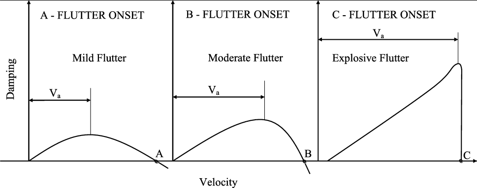
Figure 1. Damping as an indication of flutter.^{(Reference Zimmerman and Weissenburger7)}

There are several techniques to extract the frequency and damping and determine the stability of an aircraft from data obtained during flight flutter testing. Cooper^{(Reference Cooper8)} and Kayran^{(Reference Kayran9)} have reviewed various techniques that have been used to estimate modal parameters from flight flutter test data. These methods can be classified into frequency-domain methods and time-domain methods, depending upon whether the curve fitting is performed in the frequency or time domain. Frequency-domain methods—the traditional approach to modal parameter estimation—use a parameter estimation procedure based on the calculation of the frequency response function; random noise is removed through averaging. Any errors in the frequency response function estimation are passed onto the estimated modal parameters.

Time-domain methods, on the other hand, use time response data by curve fitting the impulse response function. The impulse response function is either calculated from the inverse Fourier transform of the frequency response function or the time-domain system response to an impulse excitation, or generated from the system response to an unknown random input. Time-domain modal analysis offers several advantages over frequency-domain approaches^{(Reference Kayran9)}. It does not depend on excitation or equipment needed to obtain specially designed excitation forces. Also, in general, it needs fewer response data. As the analysis is not based on frequency response function data, it can represent an alternative for analysing close vibration modes. However, time-domain modal analysis requires measured data with a very high signal-to-noise ratio. Data inaccuracy and the presence of noise can lead to computational modes in the calculation. Cooper^{(Reference Cooper8)} does not recommend any particular technique, but refers to the wide practice of linear modal analysis technique used for estimating frequency and damping. Dawson and Maxwell^{(Reference Dawson and Maxwell10)} used amplitude and velocity inputs, wherein the onset of flutter is predicted by recording the maximum amplitude data for a structure at various test points. The maximum amplitude is obtained from a sharp, adequate and precisely repeatable step excitation or by monitoring the maximum modal amplitude of a structure under the influence of a frequency sweep excitation. This technique is applied on an F-16 carrying a heavy load. Cooper^{(Reference Cooper, Emmet and Wright11)} and Dimitriadis and Cooper^{(Reference Dimitriadis and Cooper12)} used the envelope function technique, which unlike modal damping extrapolation, makes use of the envelope bounding an impulse response as obtained after a sharp impulse excitation of the structure. The size and shape of the response envelope change, reflecting the loss of damping with varying speed. Flutter instability can be predicted by extrapolating the envelope shape parameter, which reaches acertain value as flutter approaches.

Houbolt and Rainey^{(Reference Houbolt and Rainey13)} proposed the Houbolt–Rainey technique, which is essentially asubcritical response-based flutter onset prediction that can be used with either a sinusoidally varying forced excitation or a randomly varying forced excitation. The analytical foundation of this approach is straightforward and simply requires a measurement of the amplitude of the response in the structural mode that is important to flutter. The reciprocal of these amplitude measurements are plotted against a flow parameter such as density or dynamic pressure, as flutter is approached, and the resulting curve is extrapolated to the flutter condition, which occurs when the reciprocal of the amplitude becomes zero. Sandford et al.^{(Reference Sandford, Abel and Gray14)} presented some results using a subcritical response method that they called the peak-hold method. Foughner^{(Reference Foughner15)} used this method during flutter testing at the NASA Langley transonic dynamics tunnel. Doggett^{(Reference Doggett16)} examined the relationship between the Houbolt–Rainey and peak-hold method and stated that these two methods are the same, suggesting that the method be referred to in the future as the Houbolt–Rainey method.

The $$\mu$$ flutterometer method used by Brenner et al.^{(Reference Brenner, Lind and Voracek17)}, Lind^{(Reference Lind18,Reference Lind19,Reference Lind20)} and Lind and Brenner^{(Reference Lind and Brenner21, Reference Lind and Brenner22,Reference Lind and Brenner23)} provides a methodology for the computation of a worst-case estimate of flutter speed that is conservative with respect to the true flutter speed by considering the errors and uncertainty in a mathematical model. The flutterometer approach uses flight flutter test data to identify the errors and uncertainty in a model. The resulting worst-case flutter margins predicted using the $$\mu$$ flutterometer directly account for data that describe the aircraft, as distinguished from a mathematical model of the aircraft. However, this method is more conservative in predicting the flutter onset speed owing to the incorporation of uncertainty into the model.

Zimmerman and Weissenburger^{(Reference Zimmerman and Weissenburger7)} introduced the flutter margin concept based on Routh’s stability criteria. The flutter margin (FM) is computed using frequencies and modal damping values. It was developed based on a binary flutter system. The flutter margin decreases much more gradually than the damping of the critical mode. The flutter margin is also expressed as a quadratic function of the dynamic pressure. Hence, if the flutter margin is known at three different airspeeds, it can be fitted using a second-order polynomial and subsequently extrapolated to the zero flutter margin where flutter occurs. Price and Lee^{(Reference Price and Lee24)} developed a new form of flutter margin for trinary flutter that also varies linearly with dynamic pressure; it is also relatively insensitive to errors in damping, but is very sensitive to errors in frequency. However, they applied this technique to a specific case of a known trinary flutter problem, which may not always be the case. Lind^{(Reference Lind25)} introduced an extension to the Zimmerman and Weissenburger^{(Reference Zimmerman and Weissenburger7)} approach that accounts for multi-mode coupling in the flutter instability. Both the classical two-mode coupling and a multi-mode coupling approach showed similar accuracy and confidence level when the critical flutter mode was considered in the modal pairing. Torii and Matsuzaki^{(Reference Torii and Matsuzaki26)} proposed a new flutter prediction parameter based on the Jury stability criteria in the sampled time domain, which is analogous to the continuous time flutter margin defined by Zimmerman and Weissenburger^{(Reference Zimmerman and Weissenburger7)}.

Kayran^{(Reference Kayran9)} reviewed various flight flutter test techniques utilised in flight testing of aircraft. The flight test procedures typically followed in flight flutter testing are described for different airspeed regimes. Kayran^{(Reference Kayran9)} mentions that the flutter margin method can be used for systems having more than two degrees of freedom, if it is known beforehand which two modes will cause flutter. In that case, the flutter margin can be applied successfully; otherwise, all possible pairs of modes must be examined. Flutter margin-based flutter prediction was applied to the F-15 flight flutter test data by Katz et al.^{(Reference Katz, Foppe and Grossman27)}. They defined the critical flutter boundary using the flutter margin for all the important modal combinations. When using the flutter margin, the frequency and damping must be known beforehand.

System identification^{(Reference Astrom and Eykhoff28,Reference Ljung29)} is the process of determining an adequate mathematical model, usually containing differential or finite-difference equations, with unknown parameters to be determined indirectly from measured data. These techniques can be used for the estimation of the frequency, damping and stability from flight flutter test measurements. The stability can be estimated directly using flight flutter test response data without estimating the frequency and damping by using such system identification techniques.

Sundaramurthy et al.^{(Reference Sundaramurthy, Jategaonkar and Balakrishna30)} used a technique based on the flow unsteadiness as the primary excitation for dynamic stability measurements in a trisonic wind tunnel. Time series auto-regressive modelling was used to derive a digital spectrum of the unsteadiness excited model response, and the system damping was evaluated from the half-power bandwidth of the spectrum. Perangelo and Waisanen^{(Reference Perangelo and Waisanen31)} examined the capability of the maximum-likelihood technique to determine the modal frequency and damping estimates from noisy flutter response signals by comparison with least-squares flutter analysis procedures. Batill et al.^{(Reference Batill, Carey and Kehoe32)}, Pinkelman et al.^{(Reference Pinkelman, Batill and Kehoe33,Reference Pinkelman, Batill and Kehoe34)} used parameter identification time series models for linear dynamic structural systems. Total least squares provides an approach that appears to significantly reduce the bias error in the parameter estimates. These methods are applied to a simple, simulated system, and then to flight flutter test data with a particular emphasis on accurate modal damping estimates. McNamara and Friedmann^{(Reference McNamara and Friedmann35)} compared three different flutter identification methods, namely the Moving Block Approach (MBA), Least-Squares Curve-Fitting method (LSCFM) and a system identification technique using an Auto-regressive Moving-Average (ARMA) model. Using analytical data, they found the ARMA model-based prediction tool to be superior to both MBA and LSCFM. Jategaonkar and Balakrishna^{(Reference Jategaonkar and Balakrishna36)} used analytical data and a known number of modes to estimate the frequency and damping using an AR model.

Kay^{(Reference Kay37)} classified spectral estimation techniques into non-parametric and parametric methods. Non-parametric methods are referred to as classical techniques, and parametric methods as modern spectral estimation techniques. Fast Fourier Transform (FFT) methods, which are non-parametric, do not require a model or parameter estimation for the spectral estimation. The Fourier transformation operations are performed on either windowed data or windowed Auto-correlation Function (ACF) estimates. Such windowing of data or ACF values makes an implicit assumption that the unobserved data or ACF values outside the window are zero, which is normally an unrealistic assumption. A smeared spectral estimate is a consequence of windowing. AR, MA and ARMA models are parametric methods. Parametric modelling for spectral estimation consists of choosing an appropriate model, estimating the parameters of the model and then substituting these estimated values into theoretical expressions for the power spectral density (PSD). One of the promising aspects of the model-based approach to spectral estimation is that one can make more realistic assumptions concerning the nature of the measured process outside the measurement interval, beyond assuming it to be zero or cyclic. Thus, the need for window functions can be eliminated, together with their impact. Kay^{(Reference Kay and Marple38)} stated that FFT methods are inferior to the AR modelling method, as very long signal records are necessary for the spectral estimation, highlighting the advantages of modern spectral estimation techniques over classical techniques. Jategaonkar and Balakrishna^{(Reference Jategaonkar and Balakrishna36)} mention that, in blow-down tunnels, long-period records are highly uneconomical and FFT methods are not preferred for analysis.

Raol et al.^{(Reference Raol, Jategaonkar and Balakrishna39)} investigated the problem of model order determination, which is an integral part of system identification for dynamical systems using auto-regressive and least-squares techniques. Twelve model order testing criteria available in literature were critically evaluated using simulated data. The study revealed that, among all the tested criteria, only a subset are adequate to establish the model order reliably. Two criteria proposed by Akaike, namely the Final Prediction Error (FPE) and the Akaike Information Criterion (AIC)^{(Reference Akaike40,Reference Akaike41,Reference Kay37)} , are found to be more reliable. These model order estimators are based on the estimated prediction error power. Pan^{(Reference Pan42)} used the Akaike information criterion in his biomedical studies. Bozdogan^{(Reference Bozdogan43)} studied the basic underlying idea of the Akaike information criterion and introduced a new measure of complexity—the information complexity (ICOMP) criterion—as a decision rule for model selection and evaluation.

Matsuzaki and Ando^{(Reference Matsuzaki and Ando44)} suggested a system identification analysis procedure using the ARMA representation of an aeroelastic system as a means of predicting the flutter velocity. The basis for this approach is the Jury stability criteria^{(Reference Kuo45)} for evaluating the stability of a discrete system, which are very similar to Routh’s stability criterion for continuous-time systems. This was applied to binary flutter systems. The flutter prediction parameter $$F_z$$ proposed by^{(Reference Torii and Matsuzaki26)} was updated to include multiple modes by^{(Reference Bae, Matsuzaki and Inman46)}, thus defining a new parameter $$F_n$$. This technique has been applied to subsonic wind-tunnel test data. Recently, Torii^{(Reference Torii and Matsuzaki47)} described a procedure for three-mode discrete-time systems.

In the discussion that follows, we present an analysis based on simulations using five different flutter prediction methods, starting with the traditional velocity damping-based flutter prediction, followed by the envelope function-based technique, the Houbolt–Rainey approach, the flutter margin-based flutter prediction, and AR-based prediction models. The same aeroelastic system is simulated and used for flutter prediction by each of the five different techniques. The aeroelastic system has three degrees of freedom, and the flutter speed is computed for this system using the V–g method with unsteady potential flow aerodynamics resulting from a rational function approximation of Theodorsen’s function.

3.0 AEROELASTIC RESPONSE OF A WING SECTION

This section describes the flutter instability of a wing section with a control surface hinged to it. The three-degree-of-freedom model of this wing section is shown in Figure 2, where b is the semi-chord of the aerofoil section, a is the non-dimensional distance between the elastic axis and the mid-chord, and c is the non-dimensional distance between the hinge point and the mid-chord, both expressed as a ratio of the semi-chord. We first develop the equations of motion of this three-degree-of-freedom vibration model, then describe the unsteady aerodynamic terms and the flutter instability problem.

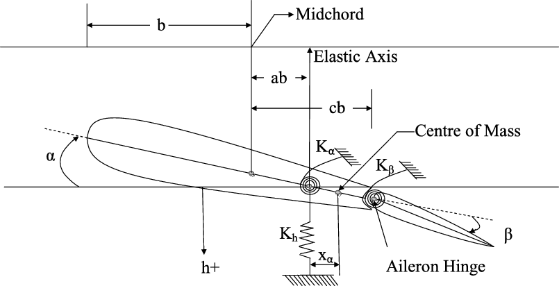
Figure 2. The three-degree-of-freedom aerofoil.

3.1 Equations of motion

The wing section model with heave, pitch and control surface degrees of freedom having linear stiffness constraints is shown in Figure 2. The heave stiffness is represented by $$K_{h}$$, the torsional stiffness of the spring is represented by $$K_{\alpha}$$ and the torsional stiffness of the control surface is represented by $$K_{\beta}$$. h is the vertical displacement of the elastic axis, positive downward; $$\alpha$$ is the angle-of-attack, positive clockwise, of the entire aerofoil, about its elastic axis; $$\beta$$ is the angular deflection, positive downward, of the control surface relative to its undisturbed position. For the three-degree-of-freedom wing section, the differential equations of motions can be written using Newton’s second law of motion^{(Reference Nam, Kim and Weisshaar1)} as follows:

(1) $\begin{equation}m\ddot{h} + S_{\alpha}\ddot{\alpha}+ S_{\beta}\ddot{\beta}+ K_{h}h = F,\end{equation}$

(2) $\begin{equation}S_{\alpha}\ddot{h} + I_{\alpha}\ddot{\alpha}+ [I_{\beta}+b(c-a)S_{\beta}]\ddot{\beta}+ K_{\alpha}\alpha = M\end{equation}$

and

(3) $\begin{equation}S_{\beta}\ddot{h}+ [I_{\beta}+b(c-a)S_{\beta}]\ddot{\alpha}+ I_{\beta}\ddot{\beta}+ K_{\beta}\beta = M_{\beta},\end{equation}$

where $$S_{\alpha}$$ = $$mx_{\alpha}$$, $$S_{\beta}$$ = $$mx_{\beta}$$, $$I_{\alpha}=mr^{2}_{\alpha}$$, $$I_{\beta}=mr^{2}_{\beta}$$.

In matrix form, these three equations can be represented as

(4) $\begin{align}&\begin{bmatrix}m\quad & \quad mx_{\alpha}\quad & \quad mx_{\beta} \\[3pt]mx_{\alpha}\quad & \quad mr^2_{\alpha}\quad & \quad mr^2_{\alpha}+ mx_{\beta}(bc-ba)\\[3pt]mx_{\beta}\quad & \quad mr^2_{\alpha} + mx_{\beta}(bc-ba)\quad & \quad mr^2_{\beta}\end{bmatrix}\begin{Bmatrix}{\ddot{h}}\\[3pt]{\ddot{\alpha}}\\[3pt]{\ddot{\beta}}\end{Bmatrix}\nonumber\\[3pt]&\quad\qquad+\left[\begin{array}{c@{\qquad}c@{\qquad}l}K_h & 0 & 0\\[3pt]0 & K_{\alpha}& 0\\[3pt]0 & 0 & K_{\beta}\end{array}\right]\begin{Bmatrix}h\\[3pt]{\alpha}\\[3pt]{\beta}\end{Bmatrix}=\begin{Bmatrix}F\\[3pt]M\\[3pt]M_{\beta}\end{Bmatrix}\!.\end{align}$

3.2 Aerodynamic forces

The unsteady aerodynamic forces are calculated based on linearised thin-aerofoil theory. In this study, Theodorsen’s approach^{(Reference Theodorsen48)} is used to calculate the aerodynamic forces and moments. Here, we follow the representation of this theory given in^{(Reference Nam, Kim and Weisshaar1)}.

The total force and moment resulting from the non-circulatory and circulatory flows are expressed as

(5) $\begin{eqnarray}\begin{array}{c@{\qquad}c@{\qquad}l}F &\!\!\!\!\!\!\!\!\! =\!\!\!\!\!\!\!\!\! & -\pi\rho b^2\left[\ddot{h} + V\dot{\alpha} - ba\ddot{\alpha} - \cfrac{V}{\pi}T_{4}\dot{\beta} - \cfrac{b}{\pi}T_{1}\ddot{\beta}\right] - 2\pi\rho VbQC(k),\\\end{array}\qquad\qquad\end{eqnarray}$

(6) $\begin{align}M & = \pi\rho b^2\Bigg[ ba\ddot{h} - Vb\left(\cfrac{1}{2}-a\right)\dot{\alpha} - b^{2}\left(\cfrac{1}{8}+a^2\right)\ddot{\alpha} - \cfrac{V^2}{\pi}\,(T_{4} + T_{10})\beta\nonumber\\[3pt]&\quad + \cfrac{Vb}{\pi}\left\{-T_{1}+T_{8}+(c-a)T_{4}-\cfrac{1}{2}T_{11}\right\}\dot{\beta} + \cfrac{b^2}{\pi} \,(T_{7}+(c-a)T_{1})\ddot{\beta}\Bigg]\\[3pt]&\quad + 2\pi\rho Vb^2\left(a+\cfrac{1}{2}\right)QC(k)\nonumber\end{align}$

(7) $\begin{align}M_{\beta} & = \pi\rho b^2\Bigg[\cfrac{b}{\pi}T_{1}\ddot{h} + \cfrac{Vb}{\pi}\left\{{2T_{9}+T_{1}-\left(a-\cfrac{1}{2}\right)T_{4}}\right\}\dot{\alpha}\nonumber\\[3pt]& \quad- \cfrac{2b^2}{\pi}T_{13}\ddot{\alpha} - \left(\cfrac{V}{\pi}\right)^2(T_{5}-T_{4}T_{10})\beta\\[3pt]& \quad+ \cfrac{Vb}{2\pi^2}T_{4}T_{11}\dot{\beta} + \left(\cfrac{b}{\pi}\right)^2T_{3}\ddot{\beta}\Bigg] - \rho Vb^2T_{12}QC(k)\nonumber\end{align}$

In the above set of equations, V is the free-stream airspeed, $$\rho$$ is the air density and C(k) is Theodorsen’s function as a function of the reduced frequency k, and is associated with the circulatory component of the unsteady forces. Q in the above is defined as

(8) $\begin{equation}Q = V\alpha + \dot{h} + \dot{\alpha}b\left(\cfrac{1}{2}-a\right)+\cfrac{V}{\pi}T_{10}\beta + \cfrac{b}{2\pi}T_{11}\dot{\beta},\end{equation}$

and the $$T_i$$ functions are given in^{(Reference Nam, Kim and Weisshaar1)} pp.16–20

Q can be rewritten in the following form by using $$S_1$$ and $$S_2$$:

(9) $\begin{eqnarray}\begin{array}{c@{\qquad}c@{\qquad}l}Q = V[S_1]{\lbrace x_s \rbrace} + b[S_2]{\lbrace{\dot{x_s}}\rbrace}\end{array}\end{eqnarray}$

where

(10) $\begin{equation}S_1 =\left[\begin{array}{c@{\qquad}c@{\qquad}l}0 & 1 & \dfrac{T_{10}}{\pi}\end{array}\right]\qquad\quad\end{equation}$

(11) $\begin{equation}S_2 =\left[\begin{array}{c@{\qquad}c@{\qquad}l}1 & (0.5-a) & \dfrac{T_{11}}{2\pi}\end{array}\right]\end{equation}$

(12) $\begin{equation}x_s =\begin{Bmatrix}h/b\\\alpha\\\beta\end{Bmatrix}\!.\qquad\qquad\qquad\quad\end{equation}$

In matrix form, the aerodynamic forces and moments will be

(13) $\begin{align}\begin{Bmatrix}F/b \\[3pt] M/b^2 \\[3pt] M_{\beta}/b^2\end{Bmatrix}&= q \Bigg[(2C(k)\lbrace R \rbrace [S_1]\lbrace {x_s} \rbrace + \cfrac{2b}{V}\,C(k) \lbrace R \rbrace [S_2] \lbrace {\dot{x_s}} \rbrace\nonumber\\& \quad+ \cfrac{2b^2}{V^2}\,[M_{nc}] \lbrace {\ddot{x_s}} \rbrace + \cfrac{2b}{V}\,[B_{nc}]\lbrace {\dot{x_s}} \rbrace + 2[K_{nc}] \lbrace x_s \rbrace \Bigg]\end{align}$

where

(14) $\begin{equation}R=\begin{Bmatrix}-2\pi \\2\pi(a+0.5)\\-T_{12}\end{Bmatrix}\end{equation}$

In the above set of equations, the subscript nc denotes the non-circulatory contribution.

(15) $\begin{equation}M_{nc} =\begin{bmatrix}-\pi \quad & \quad \pi a \quad & \quad T_1 \\[3pt]\pi a \quad & \quad -\pi\left(\dfrac{1}{8}+a^2\right) \quad & \quad -2T_{13}\\[3pt]T_1 \quad & \quad -2T_{13} \quad & \quad \dfrac{T_3}{\pi}\end{bmatrix}\end{equation}$

(16) $\begin{equation}B_{nc} =\begin{bmatrix}0 \quad & \quad -\pi \quad & \quad T_4 \\[3pt]0 \quad & \quad \pi\left(a-\dfrac{1}{2}\right) \quad & \quad -T_{16} \\[3pt]0 \quad & \quad -T_{17} \quad & \quad -\dfrac{T_{19}}{\pi}\end{bmatrix}\qquad\ \end{equation}$

(17) $\begin{equation}K_{nc} =\begin{bmatrix}0\quad & \quad0\quad & \quad0\\[3pt]0\quad & \quad0\quad & \quad-T_{15}\\[3pt]0\quad & \quad0\quad & \quad- \dfrac{T_{18}}{\pi}\end{bmatrix}\qquad\qquad\quad\ \end{equation}$

Equation (4) can now be presented as

(18) $\begin{eqnarray}\centering\begin{split}&\left[\begin{array}{c@{\qquad}c@{\qquad}c}1 & \overline{x}_{\theta} & \overline{x}_{\beta}\\[3pt]\overline{x}_{\theta} & \overline{r}^2_{\theta} & \overline{r}^2_{\theta} + \overline{x}_{\beta}(c-a)\\[3pt]\overline{x}_{\beta} & \overline{r}^2_{\theta} + \overline{x}_{\beta}(c-a) & \overline{r}^2_{\beta}\end{array}\right]\left\{\begin{array}{c}\ddot{h}/b\\[3pt]\ddot{\alpha}\\[3pt]\ddot{\beta}\end{array}\right\}+\left[\begin{array}{c@{\quad}c@{\quad}c}\omega^2_{h} & 0 & 0 \\[3pt]0 & \omega^2_{\alpha}\overline{r}^2_{\theta} & 0 \\[3pt]0 & 0 & \omega^2_{\beta}\overline{r}^2_{\beta}\end{array}\right]\left\{\begin{array}{c}h/b\\[3pt]\alpha\\[3pt]\beta\end{array}\right\}\\[3pt]&\quad=\cfrac{q}{m}\left[2C(k)\left\{\begin{Bmatrix}-2\pi\\[3pt]2\pi(a+0.5)\\[3pt]-T_{12}\end{Bmatrix}\left[\begin{array}{c@{\qquad}c@{\qquad}c}0 & 1 & \cfrac{T_{10}}{\pi}\end{array}\right]\begin{Bmatrix}h/b\\[3pt]\alpha\\[3pt]\beta\end{Bmatrix}\right.\right.\\[3pt]&\qquad+ \left.\cfrac{2b}{V}\begin{Bmatrix}-2\pi\\[3pt]2\pi(a+0.5)\\[3pt]-T_{12}\end{Bmatrix}\begin{bmatrix}1 & (0.5-a) & \cfrac{T_{11}}{2\pi}\end{bmatrix}\begin{Bmatrix}\dot{h}/b\\[3pt]\dot{\alpha}\\[3pt]\dot{\beta}\end{Bmatrix}\right\}\\[3pt]&\qquad+ \cfrac{2b^2}{V^2}\begin{bmatrix}-\pi & \pi a & T_1 \\[3pt]\pi a & - \pi\left(\cfrac{1}{8}+a^2\right) & -2T_{13} \\[3pt]T_1 & -2T_{13} & \cfrac{T_3}{\pi}\end{bmatrix}\begin{Bmatrix}\ddot{h}/b\\[3pt]\ddot{\alpha}\\[3pt]\ddot{\beta}\end{Bmatrix}\\[3pt]&\qquad+ {\cfrac{2b}{V}}\begin{bmatrix}0\quad & \quad-\pi\quad &\quad T_4\\[3pt]0\quad & \quad\pi\left(a - \cfrac{1}{2}\right)\quad & \quad-T_{16} \\[3pt]0\quad & \quad-T_{17}\quad & \quad-\cfrac{T_{19}}{\pi}\end{bmatrix}\begin{Bmatrix}\dot{h}/b\\[3pt]\dot{\alpha}\\[3pt]\dot{\beta}\end{Bmatrix}\\[3pt]&\qquad+ \left.2\begin{bmatrix}0\quad & \quad0\quad &\quad 0\\[3pt]0\quad & \quad0\quad & \quad-T_{15}\\[3pt]0\quad & \quad0\quad &\quad -\cfrac{T_{18}}{\pi}\end{bmatrix}\begin{Bmatrix}h/b\\[3pt]\alpha\\[3pt]\beta\end{Bmatrix}\right]\end{split}\end{eqnarray}$

or more compactly

(19) $\begin{align}[\overline{M}]\lbrace \ddot{x_s} \rbrace + [\overline{K}] \lbrace x_s \rbrace & = \cfrac{q}{m}\,[2C(k)\lbrace R \rbrace [S_1] \lbrace x_s \rbrace + \cfrac{2b}{V}\,C(k) \lbrace R \rbrace [S_2] \lbrace \dot{x_s} \rbrace\nonumber\\& \quad+ \cfrac{2b^2}{V^2}\,[M_{nc}] \lbrace \ddot{x_s} \rbrace +\cfrac{2b}{V}\,[B_{nc}] \lbrace \dot{x_s} \rbrace + 2[K_{nc}] \lbrace x_s \rbrace].\end{align}$

3.3 The rational function approximation of the unsteady aerodynamic forces

To transform the equations of motion into state-space form, the frequency-domain unsteady aerodynamic forces must be approximated in terms of rational functions of the Laplace variable. However, when such Rational Function Approximation (RFA) is conducted, it results in an increase in the number of augmented aerodynamic states required to accurately represent the unsteady aerodynamic forces. There are several approaches for RFA, such as the matrix Pad approximant technique^{(Reference Vepa49,Reference Edwards50)} , minimum-state method^{(Reference Karpel51-Reference Karpel and Strul53)}, corrected/modified minimum-state method^{(Reference Wang and Chen54,Reference Karpel55)} , mixed method^{(Reference Biskri, Botez, Stathopoulos, Therien, Rathe and Dickinson56)}, Chebyshev polynomials method^{(Reference Dinu, Botez and Cotoi57,Reference Botez, Dinu and Cotoi58)} and Rogers method^{(Reference Roger59)}.

In this paper, the RFA approach based on Roger’s method is used. This method is very simple and accurately transforms the unsteady aerodynamic forces from the frequency to time domain^{(Reference Nam, Kim and Weisshaar1)}. The unsteady aerodynamic forces given by Equation (13) in the frequency domain can be recast as

(20) $\begin{eqnarray}\begin{array}{ccl}\begin{Bmatrix}F/b \\[3pt]M/b^2 \\[3pt] M_{\beta}/b^2\end{Bmatrix}& = & q\Big[2C(k)\lbrace R \rbrace [S_1] + i2kC(k)\lbrace R \rbrace [S_2] - 2k^2[M_{nc}]\\[-10pt]& & + \,i2k[B_{nc}] + 2[K_{nc}]\Big]\{x_s\} \\& = & q \Big[2C(k)\lbrace R \rbrace [S_1] + is'C(k)\lbrace R \rbrace [S_2] - 2s'^2[M_{nc}]\\& & + \,i2s'[B_{nc}] + 2[K_{nc}]\Big]\{x_s\}\\& = & q[A(s')]\{x_s\}\\\end{array}\end{eqnarray}$

where s′ is the non-dimensionalised Laplace variable $$s' = sb /V$$. Let the calculated aerodynamic forces be represented as $$[A(s')] = [F(s')] + i[G(s')]$$. The real and imaginary part of the aerodynamic matrix will then be

(21) $\begin{equation}\begin{aligned}\bigl[A(s')\bigr] & = [P_{0}] + [P_{1}]s' + [P_{2}]s'^2 + \sum_{j=3}^{N}\frac{[P_j]s'}{s'+\gamma_{j-2}}; \\\Re[A(s')] & \triangleq [F(s')] = [P_{0}] + [P_{2}]s'^2 + \sum_{j-3}^{N}\frac{[P_j](-s'^2)}{(-s'^2)+\gamma_{j-2}^2},\\\Im[A(s')] & \triangleq [G(s')] = [P_{1}]s' + \sum_{j-3}^{N}\frac{[P_j]\gamma_{j-2}s'}{(-s'^2)+\gamma_{j-2}^2}.\end{aligned}\end{equation}$

$$\gamma_{j-2}$$ are the aerodynamic poles, which are usually preselected in the range of reduced frequencies of interest. The real matrices $$[P_j]$$ are determined using the least-squares technique for a term by term fitting of the aerodynamic matrix [A(s′)]. The augmented aerodynamic state is defined as

(22) $\begin{eqnarray}\{x_{aj}\} & = & \frac{s'}{s'+\gamma_{j-2}}\{x_s\} = \frac{s}{s+\frac{V}{b}\gamma_{j-2}} \end{eqnarray}$

(23) $\begin{eqnarray}\{\dot{x}_{aj}\} & = & \{\dot{x}_s\} - \frac{V}{b}\gamma_{j-2}\{x_{aj}\}\qquad\quad\end{eqnarray}$

One can now represent Equation (19), together with the unsteady aerodynamic states, because the augmented state-space equation of motion now represents a linear time-invariant system.

(24) $\begin{equation}\begin{Bmatrix}\dot{x}_s\\\ddot{x}_{s}\\\dot{x}_{a3}\\\vdots\\\dot{x}_{aN}\end{Bmatrix}=\begin{bmatrix}0 & I & 0 & \dotsb & 0\\[5pt]-\overline{M}^{-1}\overline{K} & -\overline{M}^{-1}\overline{B} & q\overline{M}^{-1}P_{3} & \dotsb & q\overline{M}^{-1}P_{N}\\[5pt]0 & I & -\left(\frac{V}{b}\right)\gamma_{1}I & \dotsb & 0\\[5pt]\dotsb & \dotsb & \dotsb & \dotsb & \dotsb\\[3pt]0 & I & 0 & 0 & -\left(\frac{V}{b}\right)\gamma_{N-2}I\end{bmatrix}\begin{Bmatrix}x_s\\\dot{x}_s\\x_{a3}\\\vdots\\x_{aN}\end{Bmatrix}\end{equation}$

where

(25) $\begin{eqnarray}\overline{M} & = & M - qP_2\left(\frac{b}{V}\right)^2 \end{eqnarray}$

(26) $\begin{eqnarray}\overline{B} & = & B - qP_1\left(\frac{b}{V}\right) \ \end{eqnarray}$

(27) $\begin{eqnarray}\overline{K} & = & K - qP_0\qquad\ \ \,\end{eqnarray}$

4.0 ANALYTICAL FLUTTER PREDICTION

We assume that the aeroelastic system is vibrating harmonically as $$x_s(t)=x_{s}e^{i\omega t}$$. Substituting into Equation 19 and re-arranging terms, we get

(28) $\begin{align}\cfrac{1}{\omega^2}\,[\overline{K}]\lbrace x_s \rbrace & = [\overline{M}]\lbrace x_s \rbrace + \cfrac{1}{\mu}\Bigg[\cfrac{1}{k^2}\,C(k)\lbrace R \rbrace [S_1]\lbrace x_s \rbrace + i \cfrac{1}{k}\,C(k)\lbrace R \rbrace [S_2] \lbrace x_s \rbrace\nonumber\\&\quad - [M_{nc}]\lbrace x_s \rbrace + i \cfrac{1}{k}\,[B_{nc}]\lbrace x_s \rbrace + \cfrac{1}{k^2}\,[K_{nc}] \lbrace x_s \rbrace \Bigg],\end{align}$

where $${\mu}$$ is the mass ratio and $$k=\omega b/V$$ is the reduced frequency. In the V–g ^{(Reference Nam, Kim and Weisshaar1)} or k method^{(Reference Wright and Cooper60)} of flutter analysis, Equation 28 is recast as a complex eigenvalue problem by introducing an artificial structural damping term g. This structural damping force is proportional to the structural stiffness but in quadrature with the displacement. Note that this structural damping is frequency independent.

(29) $\begin{align}\cfrac{1+ig}{\omega^2}\,[\overline{K}]\lbrace x_s \rbrace & = [\overline{M}]\lbrace x_s \rbrace + \cfrac{1}{\mu} \Bigg[\cfrac{1}{k^2}\,C(k)\lbrace R \rbrace [S_1] \lbrace x_s \rbrace + i \cfrac{1}{k}\,C(k) \lbrace R \rbrace [S_2] \lbrace x_s \rbrace\nonumber\\& \quad- [M_{nc}] \lbrace x_s \rbrace + i \cfrac{1}{k}\,[B_{nc}] \lbrace x_s \rbrace + \cfrac{1}{k^2}\,[K_{nc}] \lbrace x_s \rbrace \Bigg].\end{align}$

For a given value of reduced frequency $$k= \frac{\omega b}{V}$$, the eigenvalue $$ \lambda \triangleq \lambda_{Re}+i\lambda_{im} = \frac{1}{\omega^2}+i \frac{g}{\omega^2} $$ is determined, and we will have $$ \frac{1}{\lambda_{Re}}= \omega^{2}$$ and the structural damping factor $$g = \frac{\lambda_{im}}{\lambda_{Re}}$$.

A MATLAB code based on the theory developed above was written to determine the response data and to obtain the frequency and damping values for different airspeeds. The parameters for this simulation are presented in Table 1 ^{(Reference Nam, Kim and Weisshaar1)}. The different k values were obtained by varying the aircraft speed V. The response obtained at a speed of $$301.68$$ft/s corresponds to the flutter speed, and the dynamic pressure at this point is $$0.75$$psi^{(Reference Nam, Kim and Weisshaar1)}. The acceleration response data at flutter is shown in Figure 3. Similarly, the responses obtained at a speed of 200ft/s, which is less than the flutter speed, and at a speed of 305ft/s, which is more than the flutter speed, are shown in Figure 3.

Table 1 Typical section parameters for generating the response data^{(Reference Nam, Kim and Weisshaar1)}

Using this program, it becomes possible to generate the aeroelastic response at different airspeeds, which is equivalent to obtaining data from flight flutter tests. Therefore, these response simulations are assumed to provide flight flutter test data and will be used to obtain the common aeroelastic response data sets for evaluating the flutter prediction techniques such as the velocity damping, envelope function, Zimmerman–Weissenburger flutter margin, discrete-time auto-regressive modelling and modified Houbolt–Rainey approaches.

The aeroelastic response is categorised into four sets. The first set consists of the responses obtained at airspeeds of 200, 225, 250 and 275ft/s, which can be considered as representing tests at subcritical speeds. The remaining sets are around the critical flutter speed, at speeds varying from 275 to 300ft/s in steps of 5ft/s. More specifically, the second set consists of the responses obtained at airspeeds of 275, 280, 285 and 290ft/s, the third set at airspeeds of 275, 280, 285, 290 and 295ft/s and the fourth set at airspeeds of 275, 280, 285, 290, 295 and 300ft/s. This response segregation is done to study the sensitivity of the methods to the data in terms of correctly predicting the flutter speed.

The test points of all four sets are presented in Table 2. Using the response at this combination of velocities, the flutter speed prediction capability of the above-mentioned methods is demonstrated.

Figure 3. Acceleration response data. (a) Before flutter (V = 200ft/s) (b) At flutter (V = 301:68ft/s) (c)Beyond flutter (V = 305ft/s).

Table 2 Velocity and dynamic pressure data sets

5.0 FLUTTER PREDICTION USING VELOCITY DAMPING

The technique that is most commonly used to predict the onset of flutter is to extrapolate trends of modal damping. These are data-based tools, since they rely entirely on the analysis of flight measurements of the modal damping ratio with no assumption regarding the theoretical model of the specific system being tested. This approach has been used by many authors to predict flutter^{(Reference Koenig6,Reference Kehoe3,Reference Cooper8,Reference Eldred, Venkayya and Anderson61,Reference Lind19)} . The underlying idea is that the modal damping of at least one mode of vibration becomes zero at the onset of flutter. Therefore, this flutter prediction technique consists in noting the variation in the modal damping with airspeed, and extrapolating those variations to an airspeed at which the damping would become zero. This resulting airspeed is considered as the predicted flutter speed. Although the principle is quite simple, one encounters difficulty in practice. One area of difficulty is the extraction of the modal damping. Flight test data often have low signal-to-noise ratios, hence sophisticated techniques such as parameter estimation or modal filtering may be required. Another area of difficulty is extrapolation. The damping can be a highly nonlinear function of airspeed, thus the extrapolation must be performed carefully to ensure that it accounts for any higher-order nonlinearity. Below, we outline the approach.

The equations of motion for a two-degree-of-freedom aerofoil are given as

(30) $\begin{eqnarray} \left[K_{ij}\right]\begin{Bmatrix}\frac{h}{b} \\[3pt]\alpha \end{Bmatrix}& = & \omega^2\left[A_{ij}+M_{ij}\right]\begin{Bmatrix}\frac{h}{b} \\[3pt]\alpha \end{Bmatrix},\end{eqnarray}$

where $$K_{ij}$$ is the stiffness matrix, $$M_{ij}$$ is the mass matrix and $$A_{ij}$$ is the aerodynamic matrix. The terms in the aerodynamic matrix are a function of the reduced frequency k. The velocity damping or V–g technique for determining flutter^{(Reference Fung62)} assumes a structural or hysteretic damping parameter g, such that $$\left[K_{ij}\right]$$ is replaced by $$\left( 1+ig \right) \left[ K_{ij}\right]$$. For a given reduced frequency $$k=\frac{\omega b}{V}$$, Equation (30) becomes a complex eigenvalue problem

(31) $\begin{eqnarray}\left(1+ig\right)\frac{\omega^2_\alpha}{\omega^2}\left[K_{ij}\right]\begin{Bmatrix}\frac{h}{b}\\[3pt]\alpha \end{Bmatrix}& = & \left[A_{ij}+M_{ij}\right]\begin{Bmatrix}\frac{h}{b}\\[3pt]\alpha\end{Bmatrix}\!.\end{eqnarray}$

The matrices $$A_{ij}$$, $$M_{ij}$$ and $$K_{ij}$$ are functions of the reduced frequency k. The eigenvalue, $$\lambda=(1+ig)\frac{\omega^2}{\omega^2_\alpha}$$, for a given value of k is computed, and the ratio of the real to the imaginary value of the eigenvalue, $$g=\frac{\lambda_I}{\lambda_R}$$, is varied as a function of $$\lambda_R = \frac{\omega^2}{\omega^2_\alpha}$$ for each reduced frequency. The plot of g as the ordinate and V as the abscissa, for each eigenvalue, is known as the V–g plot. The value of V at which $$g=0$$ is the flutter speed, because the effective damping at this airspeed is zero and the system is in a state of neutral dynamic equilibrium.

For each airspeed, the effective damping g is determined; the closer this damping is to zero, the closer the aeroelastic system is to flutter instability. One can extrapolate the flutter speed from off-flutter damping values and airspeeds. This is the basis of the velocity-damping technique for predicting flutter speed.

Now, referring back to Equation 29, the complex eigenvalue problem is solved by starting with large values of k; then the unsteady aerodynamic terms for the assumed value of k are looked up, and finally the eigenvalues are solved. The reciprocal of the real part of the eigenvalue gives the frequency of oscillation $$\omega^2$$, while the imaginary part gives the damping parameter g. Once the frequency of oscillation $$\omega$$ is determined, the corresponding airspeed V is known. One then plots $$\omega$$ versus V and g versus V. This procedure is then repeated with decreasing values of k until the imaginary part of the eigenvalue, or g, becomes zero. This corresponds to the flutter condition. The corresponding real part of the eigenvalue gives the flutter frequency $$\omega_f^2$$, and this together with k gives the flutter velocity $$V_f$$. The V–g method derives its name from the graph of the total aeroelastic system damping g versus airspeed, and from the fact that the flutter condition corresponds to the point on this graph where the aeroelastic system damping crosses the V axis.

Flutter prediction is carried out using the different data sets, and the results are tabulated below. The frequency and damping for various airspeeds corresponding to three modes are presented in Table 3. From this table, it can be observed that the artificial damping values are negative for all three modes, implying that the aeroelastic system is stable at these airspeeds. The procedure to predict the flutter speed using the different data sets is explained below.

Table 3 Frequency and damping values at different speeds

The damping values estimated at these data points are extrapolated to the zero damping value, and the speed corresponding to zero damping is taken as the flutter speed. The quadratic extrapolation method is used for the extrapolation. Figure 4(a) shows the variation of the damping with velocity for this case. From this plot, it is seen that the flutter velocity is $$410.20$$ft/s. This predicted flutter speed is very high compared with the theoretical value of $$301.68$$ft/s^{(Reference Nam, Kim and Weisshaar1)}. Figure 4(b) shows the variation of the damping with velocity corresponding to data set 2. From this figure, it is seen that the flutter velocity is $$316.0$$ft/s. This predicted flutter speed is closer to the theoretical value of $$301.68$$ft/s. Similar procedures are adopted for data set 3 and data set 4 for the flutter prediction and are shown in Figure 4(c) and Figure 4(d), respectively. Data set 3 predicts a flutter speed of $$309.5$$ft/s, whereas data set 4 predicts a flutter speed of $$303.2$$ft/s. Therefore, the data sets at airspeeds closer to the flutter speed predict the flutter onset speed more accurately than those that are further away.

Figure 4. Flutter prediction with the V − g method. (a) Damping g versus velocity—data set 1 (b) Damping g versus velocity—data set 2 (c) Damping g versus velocity—data set 3 (d) Damping g versus velocity—data set 4.

6.0 FLUTTER PREDICTION WITH THE ENVELOPE FUNCTION

The envelope function^{(Reference Cooper, Emmet and Wright11)} was originally proposed as a tool to provide a quick assessment of the overall aeroelastic stability to complement standard flutter prediction analysis. The basis of this technique is that the impulse response of any stable damped system decays, with the shape of the decay in the time domain being described by the decay envelope. As the damping in a given aeroelastic system decreases, the decay envelope grows wider, eventually becoming a rectangle as the damping becomes zero. Evaluation of the position of the centroid of the decay envelope and the way that it shifts on the time axis as the damping decreases enables an assessment of the stability of the system. For an aeroelastic system with an impulse response of y(t), the decay envelope, or envelope function^{(Reference Cooper, Emmet and Wright11)}, is given by

(32) $\begin{equation}\text{env}(t) = \sqrt{\left(y(t)\right)^2 + \left(y_H(t)\right)^2},\end{equation}$

where $$y_H(t)$$ is the Hilbert transform of the impulse response defined as

(33) $\begin{equation}y_H(t) = F^{-1}\left\lbrace Im[Y(\omega)] - jRe[Y(\omega)] \right\rbrace,\end{equation}$

where $$Y(\omega)$$ is the Fourier transform of y(t), Im and Re are the imaginary and real part, respectively, and $$F^{-1}$$ is the inverse Fourier transform. The time centroid of the decay envelope is given by

(34) $\begin{eqnarray}\bar{t} &=& \frac{\int_{0}^{t_{max}}env(t)tdt}{\int_{0}^{t_{max}}env(t)dt}.\end{eqnarray}$

The upper limit of the integration, $$t_{max}$$, serves to define the rectangle within which the integration takes place. For a single-degree-of-freedom system, when the damping is zero, the time centroid lies at $$t = t_{max}/2 $$. For a multi-degree-of-freedom system, it is suggested that $$t\approx t_{max}/2$$ is an adequate approximation for the position of the time centroid. Since $$\bar{t}$$ tends to increase as the damping drops, its inverse is usually employed as the significant shape parameter, that is

(35) $\begin{eqnarray}S &=& \frac{1}{\bar{t}}.\end{eqnarray}$

In that case, the value of S at the flutter condition is $$S=2/t_{max}$$ for a single-degree-of-freedom system. For a multi-degree-of-freedom system,

(36) $\begin{eqnarray} S & \approx & \frac{2}{t_{max}}.\end{eqnarray}$

The flutter testing procedure based on the envelope function evaluates S at a number of sub-critical airspeeds. The variation of S with airspeed is then curve-fit using a polynomial, as is done in the case of the velocity damping technique for flutter prediction, and extrapolated to the point where $$S=2/t_{max}$$, thus yielding the flutter velocity.

Note that this tool is not intended to replace any flutter prediction methods, but rather to provide a quick indication of whether there has been any significant change in stability since the previous test points. In this study, the shape parameter corresponding to the four data sets is computed and presented in Table 4.

Table 4 Velocity and shape parameter values

The response from data set 1 is used to estimate the shape parameters. Usually, the shape parameter values estimated at these data points are extrapolated to the shape parameter $$S=2/t_{max}$$, and the speed corresponding to this value is taken as the flutter speed. However, in this case, it is observed that the shape parameter values are increasing with velocity and do not show any tendency for flutter. This is shown in Figure 5(a). Similarly for data set 2, the shape parameters are computed and plotted with respect to velocity in Figure 5(b). From this figure, it is seen that the shape parameters show a tendency towards flutter. The predicted flutter speed is $$303.15$$ft/s. The variation of the shape parameter values with velocity using data set 3 is shown in Figure 5(c). The plot indicates a decrease in the shape parameter as the velocity increases. This trend when extrapolated to the shape parameter $$S=2/t_{max}$$ thus yields the flutter speed. The predicted flutter speed is $$300.16$$ft/s. The response from data set 4 is used to estimate the shape parameters. These shape parameters are plotted against velocity in Figure 5(d), showing a decreasing trend of the shape parameter with increasing velocity. The predicted flutter speed is $$300.71$$ft/s, and this value is close to the actual flutter speed.

Figure 5. Flutter prediction with the envelope function method. (a) Envelope function method—data set 1 (b) Envelope function method—data set 2 (c) Envelope function method—data set 3 (d) Envelope function method—data set 4.

Therefore, the envelope function technique can predict a flutter speed very close to the actual flutter speed, except for data set 1.

7.0 THE HOUBOLT–RAINEY METHOD

The Houbolt–Rainey method^{(Reference Houbolt and Rainey13,Reference Doggett16)} is a subcritical response method for flutter onset prediction that can be used with either sinusoidally or randomly varying forced excitation. The analytical foundation of this technique is straightforward and simply requires the measurement of the amplitude of the response in the structural mode that is important for flutter. Houbolt and Rainey used a classical autospectrum to determine the amplitude. The amplitude values needed by the Houbolt–Rainey method are determined by taking the r.m.s. value of the spectrum of the autocorrelation of the response. The auto-regressive spectrum of the system is given by Equation (37)^{(Reference Jategaonkar and Balakrishna36)}.

(37) $\begin{equation}\displaystyle \Phi_{AR}(\omega)=\frac{\Delta t\sigma^{2}}{1+\displaystyle\sum_{p=1}^{n}a_pe^{ip\omega\Delta t}}.\end{equation}$

The reciprocal of these amplitude measurements is plotted against velocity, and the resulting curve is extrapolated to the flutter condition, which occurs when the reciprocal of the amplitude becomes zero.

To study the effectiveness of this technique for predicting the flutter speed, the absolute value of the reciprocal of the amplitude is computed for the different data sets and shown in Table 2. The reciprocal of the amplitude values estimated at these data points is extrapolated to a zero value of the reciprocal of amplitude, and the speed corresponding to this point is taken as the flutter speed. Quadratic extrapolation is used.

The response from data set 1 is used to estimate the absolute values of the reciprocal of amplitude. These values are plotted against velocity in Figure 6(a). From this figure, it is observed that the amplitude values do not show any tendency towards flutter. Similarly, the reciprocal of the amplitude corresponding to data set 2 is estimated and plotted with respect to velocity in Figure 6(b). From this figure, it is observed that the amplitude values show a tendency towards flutter. The flutter speed predicted using this approach is 321ft/s. This value shows a large deviation from the theoretical estimation of the flutter speed. For data set 3, the reciprocal of the amplitude is estimated and plotted with respect to velocity in Figure 6(c). From this figure, it is observed that the amplitude values show a tendency towards flutter. The predicted flutter speed is $$312.5$$ft/s, showing a large deviation from the theoretical estimation of the flutter speed. Data set 4 is used to estimate the absolute value of the reciprocal of the amplitude. The absolute value of the reciprocal of the amplitude is plotted against velocity in Figure 6(d). The predicted flutter speed after extrapolation is $$304.89$$ft/s. These values tend towards the actual flutter speed of $$301.68$$ft/s.

Figure 6. Flutter prediction with the Houbolt–Rainey method. (a) Houbolt–Rainey method—data set 1 (b) Houbolt–Rainey method—data set 2 (c) Houbolt–Rainey method—data set 3 (d) Houbolt–Rainey method—data set 4.

The Houbolt–Rainey method does not predict the exact flutter speed, even from the response data close to the theoretical flutter speed. However, it predicts the tendency for flutter for response data close to the actual or theoretical flutter speed.

8.0 FLUTTER PREDICTION USING THE FLUTTER MARGIN

The flutter margin (FM) is a technique to predict the flutter onset speed^{(Reference Zimmerman and Weissenburger7)}. This method makes use of both modal frequency and damping information for two pre-identified critical modes to calculate the flutter margin. This technique is based on Routh’s stability criteria. Using the flutter margin information computed for off-flutter flight conditions, it is possible to predict the flutter onset. The basic concepts and analytical development of the flutter margin technique presented here are based on a two-degree-of-freedom aeroelastic system that represents a bending–torsion idealisation of an aircraft wing^{(Reference Hancock, Wright and Simpson63)}. Since most cases of flutter, even for multi-degree-of-freedom systems, occur as a result of the interaction between two dominant degrees of freedom, this technique is valid for multi-degree-of-freedom systems too. The system possesses a translational inertia represented by $${m}$$ and a rotational inertia represented by $${I_{c}}$$, and is subjected to a translational elastic restraint $${k_{h}}$$ and a rotational elastic restraint $${k_{\alpha}}$$ about the elastic axis. The aerodynamic forces acting on the system are with reference to the centre of mass of the aerofoil and consist of the lift force L and pitching moment $${M_{c}}$$. The aerodynamic forces are assumed to be of the form

(38) $\begin{equation}\begin{array}{ccl}L&\!=\!&C_{L_\alpha}q\left[a_1\alpha+a_2\left(\frac{\dot{h}}{V}\right)+a_3\left(\frac{\dot{\alpha}}{V}\right)\right], \\[6pt] M_c&\!=\!&C_{L_\alpha}q\left[b_1\alpha+b_2\left(\frac{\dot{h}}{V}\right)+b_3\left(\frac{\dot{\alpha}}{V}\right)\right].\end{array}\end{equation}$

The lift force and pitching moment are proportional to the dynamic pressure q, angle-of-attack $${\alpha}$$, heave velocity $$\dot{h}$$ and pitching velocity $$\dot{\alpha}$$. Substituting the expression for the aerodynamics in Equation (38) into the equations of motion in Equation (39) results in aset of simultaneous linear differential equations in the two unknowns $$\alpha$$ and h with constant coefficients. The constants $$a_{i}$$ and $$b_{i}$$ represent quasi-steady aerodynamic terms. The equations of motion become

(39) $\begin{equation}\begin{aligned}& m\ddot{h}+C_{L_\alpha}qa_2\left(\frac{\dot{h}}{V}\right)+k_hh+C_{L_\alpha}qa_3\left(\frac{\dot{\alpha}}{V}\right)+(C_{L_\alpha}qa_1-k_hx)\alpha=0, \\& I_c\ddot{\alpha}-C_{L_\alpha}qb_3\left(\frac{\dot{\alpha}}{V}\right)+(k_\alpha+k_hx^2-C_{L_\alpha}qb_1)\alpha-C_{L_\alpha}q_2\left(\frac{\dot{h}}{V}\right)-(k_hx)h=0.\end{aligned}\end{equation}$

The solution to such a set can be represented in the form

(40) $\begin{equation}\begin{aligned}& h=h_{0}e^{st} \quad \text{and} \quad \alpha=\alpha_{0}e^{st},\end{aligned}\end{equation}$

where $$h_{0}$$ and $$\alpha_{0}$$ are arbitrary integration constants and s represents the eigenvalues determined by substituting Equation (40) into the simultaneous differential Equation (39). This results in a quartic equation in s

(41) $\begin{equation}(s^4+A_3s^3+A_2s^2+A_1s+A_0)=0.\end{equation}$

The coefficients $$A_0-A_3$$ take the form

(42) $\begin{equation}\begin{aligned}A_0&=K_{01}(C_{L_\alpha}q)+K_{02}, \\A_1&=K_{11}\left(\frac{C_{L_\alpha}q}{V}\right)^2+K_{12}\left(\frac{C_{L_\alpha}q}{V}\right)\!, \\A_2&=K_{21}\left(\frac{C_{L_\alpha}q}{V}\right)^2+K_{22}C_{L_\alpha}q+K_{23}, \\A_3&=K_{31}\left(\frac{C_{L_\alpha}q}{V}\right).\end{aligned}\end{equation}$

The $$K_{ij}$$ are defined as

(43) $\begin{equation}\begin{array}{ccl}K_{01}&\!=\!&\cfrac{k_h(a_1x-b_1)}{mI_c},\\[10pt]K_{02}&\!=\!&\cfrac{k_hk_\alpha}{mI_c},\\[10pt]K_{11}&\!=\!&\cfrac{a_1b_2-a_2b_1}{mI_c},\\[10pt]K_{12}&\!=\!&\cfrac{a_2(k_\alpha+k_hx^2)+k_hx(a_3-b_2)-k_hb_3}{mI_c},\\[10pt]K_{21}&\!=\!&\cfrac{a_2b_3+a_3b_2}{mI_c},\\[10pt]K_{22}&\!=\!&\cfrac{-b_1}{I_c},\\[10pt]K_{23}&\!=\!&\left(\cfrac{k_h}{m}\right)+\cfrac{k_\alpha+k_hx^2}{I_c},\\[10pt]K_{31}&\!=\!&\cfrac{a_2}{m}-\cfrac{b_3}{I_c}.\end{array}\end{equation}$

The flutter margin is derived by applying the Routh stability criterion^{(Reference Kuo45)} to the two-mode system. This criterion is algebraic and provides information on the absolute stability of a linear time-invariant system that has a characteristic equation with constant coefficients. The Routh–Hurwitz criterion represents an algorithm for determining the location of zeros of a polynomial with constant real coefficients with respect to the left and right half of the s-plane without actually solving for the zeros. In a rather direct manner, Routh’s criterion for a system to be stable requires that all the coefficients of the characteristic equation be positive, and, furthermore, for the specific case of a quartic equation, the following relation exist between the coefficients:

(44) $\begin{equation}A_2(A_1/A_3)-(A_1/A_3)^2-A_0>0,\end{equation}$

or in a modified form

(45) $\begin{equation}\left[\left(\frac{A_2}{2}\right)^2-A_0\right]-\left[\frac{A_2}{2}-\frac{A_1}{A_3}\right]^2>0.\end{equation}$

For the system to be stable, all the A’s must be positive and the inequality of Equation (45) must be satisfied. Instability occurs when the inequality is reversed. We can define F as a flutter stability parameter

(46) $\begin{equation}F=\left[\left(\frac{A_2}{2}\right)^2-A_0\right]-\left[\frac{A_2}{2}-\frac{A_1}{A_3}\right]^2.\end{equation}$

F must be positive for stability to exist; the more positive it is, the greater the degree of stability. F as defined here is a measure of the system stability as expressed in the Routh criterion. Since the A’s vary with airspeed, the value of F will also depend upon airspeed. Its numerical value at any given speed can be considered as the flutter stability margin, and we refer to F as the flutter margin.

We designate the four roots of the characteristic Equation (41) as $$s_1$$, $$s_2$$, $$s_3$$ and $$s_4$$ such that

(47) $\begin{equation}\begin{array}{ccl}s_{1,2}&=&\beta_{1}\pm i\omega_1,\\s_{3,4}&=&\beta_{2}\pm i\omega_2,\end{array}\end{equation}$

where the $$\omega_i$$’s represent the system frequencies and the $$\beta_i$$’s represent the negative of the system decay rates. The A’s can be represented in terms of the $$\beta_i$$’s and $$\omega_i$$’s, and these are introduced into Equation (46) to yield the flutter margin

(48) $\begin{align}F & =\left[\left(\dfrac{{\omega_2}^2-{\omega_1}^2}{2}\right)+\left(\dfrac{{\beta_2}^2-{\beta_1}^2}{2}\right)\right]^2+4\beta_1\beta_2\left[\left(\dfrac{{\omega_2}^2+{\omega_1}^2}{2}\right)+2\left(\dfrac{{\beta_2}+{\beta_1}}{2}\right)^2\right]\nonumber\\& \quad-\left[\left(\dfrac{{\beta_2}-{\beta_1}}{{\beta_2}+{\beta_1}}\right)\left(\dfrac{{\omega_2}^2-{\omega_1}^2}{2}\right)+2\left(\dfrac{{\beta_2}+{\beta_1}}{2}\right)^2\right]^2.\end{align}$

Using this equation, it is possible to evaluate the flutter margin corresponding to any airspeed by measuring frequencies and damping coefficients corresponding to that speed. The flutter margin equation can be used to evaluate the flutter margin at test speeds at which the aircraft has already flown. It makes no statement about what lies beyond. Substituting the A’s defined by Equation (42) into Equation (46), the resulting equation takes the form

(49) $\begin{equation} F=B_2(C_{L_\alpha}q)^2+B_1(C_{L_\alpha}q)+B_0,\end{equation}$

where the coefficients are

(50) $\begin{equation}\begin{array}{ccl}B_2&=& \dfrac{K_{11}}{K_{31}}\left(\dfrac{K_{11}}{K_{31}}+K_{22}\right)+\dfrac{\rho C_{L_\alpha}}{2}\left(\dfrac{K_{11}K_{21}}{K_{31}}\right)\!, \\[10pt]B_1&=&\dfrac{1}{K_{31}}\left(K_{12}K_{22}+K_{11}K_{23}-2\dfrac{K_{11}K_{12}}{K_{31}}\right)-K_{01}+\dfrac{\rho C_{L_\alpha}}{2}\left(\dfrac{K_{12}K_{21}}{K_{31}}\right)\!,\\[10pt]B_0&=&\dfrac{K_{12}}{K_{31}}\left(K_{23}-\dfrac{K_{12}}{K_{31}}\right)-K_{02}.\end{array}\end{equation}$

Equation (49), expressing the parabolic variation of F with $$C_{L_\alpha}q$$, is referred to as the flutter prediction equation. The coefficients $$B_0$$, $$B_1$$ and $$B_2$$ are functions of aeroelastic parameters. The effect of $$C_{L_\alpha}$$ is captured by using flight test data corresponding to the subsonic or supersonic flight test regimes. The $$B_i$$’s are evaluated after inverting Equation (49) from the measured off-flutter test points for which the flutter margin F, $$C_{L_\alpha}$$ and q are known. Once the coefficients are determined, the $$C_{L_\alpha}q$$ corresponding to $$F=0$$ is determined by extrapolation.

In the case of the flutter margin technique, the modal combination plays a critical role in predicting the flutter speed. By selecting the combination of modes carefully, one can predict the onset of flutter speed accurately. The flutter margin is estimated using the frequency and damping values for the first three data sets as mentioned for the other flutter prediction techniques. However, the flutter margin is not estimated for the fourth set, as the other three sets are able to demonstrate the flutter prediction efficiently. To determine the flutter onset speed, the modes must be combined in pairs. The modal pair showing the lowest flutter margin is considered as to be the critical modal combination. The different modal combinations considered in this study are presented in Table 5.

Table 5 Details of the combination of the modes

The frequency and damping estimations corresponding to data set 1 are used to compute the flutter margin. The flutter margin estimated using data set 1 is plotted against velocity in Figure 7 for all three mode combinations. It is observed that the pitch and heave mode combination is the critical mode combination, and it exhibits a classical flutter phenomenon. The second modal combination, where the wing pitching mode interacts with the control surface mode, also follows the familiar control surface flutter mode combination. The third modal combination of heaving with the control surface mode does not produce any flutter instability. It is seen that the flutter margin shows an instability trend from the starting velocity. The critical mode combination which leads to flutter is shown in Figure 7(b). The flutter onset speed is estimated to be $$299.50$$ft/s.

Figure 7. Flutter prediction with the flutter margin method. (a) Variation of flutter margin against velocity (b) Flutter onset velocity for a critical mode combination (c) Variation of flutter margin against velocity (d) Flutter onset velocity for a critical mode combination (e) Variation of flutter margin against velocity (f) Flutter onset velocity for a critical mode combination.

Similarly, the frequency and damping estimations corresponding to data set 2 are used to compute the flutter margin, which is plotted against velocity in Figure 7(c). As predicted in the previous case, the pitch and heave mode combination is the critical mode combination. It is observed that the flutter margin shows instability from the beginning. However, the velocity damping approach does not show any instability or reduction in damping until a velocity of 280ft/s is reached, for the wing pitching mode. The critical mode combination which leads to flutter is shown in Figure 7(d). The flutter onset speed is estimated to be $$302.50$$ft/s. The flutter margin estimated using data set 3 is shown in Figure 7(e). As in the previous two cases, it is found that the pitch and heave mode combination is the critical mode combination. The flutter onset speed (Figure 7(f)) of $$301.4$$ft/s estimated using this data set is very close to the theoretical flutter speed. The flutter margin method is thus able to predict the onset of flutter even when using the data set lying far below the flutter onset speed. Hence, the data set closer to the flutter onset is redundant and data set 4 is not used.

9.0 FLUTTER PREDICTION USING THE AUTO-REGRESSIVE MODEL

Auto-regressive models are finite-difference models. As the flutter instability prediction relies on time-domain measurements of the system response, auto-regressive models are suitable as they are constructed from discrete-time response sequences. The stability in the constructed auto-regressive model is based on Jury’s stability criteria. The stability boundary is estimated using Jury’s stability determinants, which are expressed in terms of auto-regressive coefficients. The auto-regressive method for flutter prediction consists of two parts. The first part is the identification of the aeroelastic system as an auto-regressive model from the sampled time response and estimation of parameters. The second part consists of an estimation of the flutter prediction parameter based on Jury’s stability criteria using the estimated auto-regressive coefficients.

The auto-regressive model identification consists of three steps, namely the selection of a suitable model for the data, the selection of a suitable model order for the model, and the estimation of parameters. An AR process of order p can be represented as

(51) $\begin{equation}x[n] = - \sum_{k=1}^{p} a[k]x[n-k] + u [n]\end{equation}$

This process is termed auto-regression as the sequence $$x\left[n\right]$$ is a linear regression on itself with u[n] representing the error. Using this model, the present value of the process is expressed as a weighted sum of past values plus a noise term. The parameters a[k] are termed the auto-regressive coefficients.

The z transform of the auto-regressive model can be represented as

(52) $\begin{equation}A(z) = \sum_{k=0}^{p} a[k]z^{-k} = 1+ a[1]z^{-1}+a[2]z^{-2}+...+a[p]z^{-p}.\end{equation}$

The selection of the model order in the AR spectral estimation is a crucial step. If the selected model order is too low, it results in a smoothed estimate, whereas if it is too large, it causes spurious peaks and general statistical instability. All model order estimators are based on the estimated prediction error power. The estimated prediction error power is guaranteed to decrease or remain the same as the model order increases for all AR parameter estimation methods. Two methods are the Final Prediction Error (FPE) and Akaike Information Criterion (AIC)^{(Reference Akaike40,Reference Akaike41,Reference Kay37,Reference Sundaramurthy, Jategaonkar and Balakrishna30,Reference Raol, Jategaonkar and Balakrishna39)} . The optimised model order is the one with the minimum FPE, defined as

(53) $\begin{equation}{FPE(K)=\frac{N+K}{N-K}\rho_k},\end{equation}$

where $$\rho_k$$ is the estimate of the white noise variance, or the prediction error power, for the $$k^{th}$$-order auto-regressive model and N is the number of data points. It is seen that, although $$\rho_k$$ decreases with k, the term $$\frac{N+K}{N-K}$$ increases with k. The final prediction error is an estimate of the prediction error power when the prediction coefficients must be estimated from the data. The term $$\frac{N+K}{N-K}$$ accounts for the increase in the variance of the prediction power estimator due to inaccuracies in the prediction coefficient estimates.

A second criterion is the Akaike Information Criterion (AIC), which is defined as

(54) $\begin{equation}{AIC(K)=N\ln\rho_k+2k}.\end{equation}$

The model order selected is the one that minimises the AIC. The performance of the Akaike information criterion and final prediction error is similar. For short data records, the use of the Akaike information criterion is recommended. For larger data records, both estimators will yield identical model order estimates, since they are functionally related to each other. An important feature of the auto-regressive model description is that it has predictor capability in that, given the history of the system, the subsequent output can be predicted.

There is a direct correspondence between the auto-regressive parameters and the covariance function of the response, and this correspondence can be inverted to determine the auto-regressive parameters or coefficients from the autocorrelation function. This is done using the Yule–Walker equations. Multiplying Equation (51) by $$x[n-k]$$ and taking the expectation of the product gives

(55) $\begin{equation}r_{xx}[k] =-\sum_{l=1}^{p} a[l]r_{xx}[k-l] + r_{xu}[k-l],\end{equation}$

where $$r_{xu}[k]=E(u[n]x[n-k])$$. But $$r_{xu}=0$$ for $$k > 0$$ and $$r_{xu}=\sigma^{2}$$ for $$k=0$$. Therefore

(56) $\begin{equation}r_{xx}[k] =\begin{cases}{-\displaystyle\sum_{l=1}^{p} a[l]r_{xx}[k-l]} & \text{for $k \geq 1$},\\[4pt] -\displaystyle\sum_{l=1}^{p} a[l]r_{xx}[-l]+\sigma^2 & \text{for $k = 0$}.\end{cases}\end{equation}$

Equations (56) are the Yule–Walker equations. They define a nonlinear relationship between the parameters of an AR process and the autocorrelation function. The Yule–Walker equations in matrix form are given by

(57) $\begin{equation}\begin{bmatrix}r_{xx}[0] \quad & \quad r_{xx}[-1] \quad & \quad \cdots \quad & \quad r_{xx}[-(p-1)]\\[3pt]r_{xx}[1] \quad & \quad r_{xx}[0] \quad & \quad \cdots \quad & \quad r_{xx}[-(p-2)]\\[3pt]\vdots \quad & \quad \vdots \quad & \quad \vdots \quad & \quad \vdots \\[3pt]r_{xx}[p-1] \quad & \quad r_{xx}[p-2] \quad & \quad \cdots \quad & \quad r_{xx}[0]\\[3pt]\end{bmatrix}\begin{bmatrix}a[1]\\[3pt]a[2]\\[3pt]\vdots\\[3pt]a[p]\end{bmatrix}= -\begin{bmatrix}r_{xx}[1]\\[3pt]r_{xx}[2]\\[3pt]\vdots\\[3pt]r_{xx}[p]\end{bmatrix}\end{equation}$

In this study, the auto-regressive parameters are estimated using the MATLAB system identification toolbox^{(Reference Ljung64)}.

The flutter prediction parameter based on Jury’s stability criteria is calculated algebraically from the auto-regressive coefficients of the estimated auto-regressive model. The system under consideration is stable if Jury’s stability criterion^{(Reference Jury65)} is satisfied. A discrete-time system is stable if and only if all the characteristic roots are located inside the unit circle in the Gauss plane. Jury’s determinant method judges the stability of a discrete-time system based on the characteristic polynomial without solving for the roots. Suppose that the characteristic equation of the discrete system is given by

(58) $\begin{equation}G(z)=A_{n}z^n+A_{n-1}z^{n-1}+\ldots+A_1z+A_0,\end{equation}$

where n is an even number and $$A_i$$ are the coefficients of the characteristic polynomial. Then the necessary and sufficient conditions for the system to be stable are that all of the following parameters are positive:

(59) $\begin{align}G(1) &= A_n + A_{n-1} + \cdots + A_1 + A_0, \nonumber\\G(-1) &= A_n - A_{n-1} + \cdots + A_1 + A_0,\nonumber \\F^+(k) &= \text{det}(X_k + Y_k) \quad k=1,3,\cdots , n-1, \\F^-(k) &= \text{det}(X_k - Y_k) \quad k=1,3,\cdots , n-1\nonumber\end{align}$

where $$X_k$$ and $$Y_k$$ are matrices whose elements consist of the coefficients of Equation (58)

(60) $\begin{equation}X_k=\left[\begin{array}{c@{\qquad}c@{\qquad}l}A_n\cdots&\cdots& A_{n-k+1}\\0 &\cdots&\cdots\\0 & 0 & A_n, \\\end{array}\right]\!, \quad Y_k=\left[\begin{array}{c@{\qquad}c@{\qquad}l}A_{k-1} & \cdots & A_0 \\\cdots & \cdots & 0 \\A_0 & 0 & 0 .\\\end{array}\right]\\\end{equation}$

Among these parameters, $$F^-(n-1)$$ can be expressed by means of characteristic roots as

(61) $\begin{equation}F^-(n-1)=A_n^{n-1}\prod_{i<j}(1-z_iz_j) = \text{det}(X_{n-1}-Y_{n-1}).\end{equation}$

Therefore, $$F^-(n-1)$$ becomes zero whenever any pair of complex-conjugate characteristic roots reaches the unit circle, which is the stability boundary.

$$F^-(n-1)$$ is called the stability parameter and is utilised for flutter prediction. Although $$F^-(n-1)$$ is a better index for flutter prediction than the modal damping, its behaviour against dynamic pressure is inferior to that of the flutter margin. To overcome this drawback, Torii^{(Reference Torii and Matsuzaki47)} proposed a flutter prediction parameter that is linearly related to the dynamic pressure. To predict the flutter boundary of a multi-mode system, the flutter prediction parameter $$F_N$$ is

(62) $\begin{equation}\begin{array}{c@{\qquad}c@{\qquad}l}F_N = \dfrac{F^-(n-1)} {\left(F^-(n-2)\right)^{2}},\end{array}\end{equation}$

where $$F^-(n-1)$$ and $$F^-(n-2)$$ are defined by Equations (61). For a binary flutter system, a fourth-order characteristic polynomial

(63) $\begin{equation}{G(z)=A_4z^4+A_3z^3+A_2z^2+A_1z+A_0},\end{equation}$

should be estimated, where $$A_0$$, $$A_1$$, $$A_2$$, $$A_3$$ and $$A_4$$ are the auto-regressive coefficients. Jury’s stability criterion simplifies to

(64) $\begin{equation}\begin{aligned} G(1)&=A_4+A_3+A_2+A_1+A_0 > 0, \\[4pt] G(-1)&=A_4-A_3+A_2-A_1+A_0>0, \\[4pt] F^+(1)&=A_4+A_0 > 0, \\[4pt] F^-(1)&=A_4-A_0 > 0, \\[4pt] F^+(3)&=|X_3+Y_3|>0, \\[4pt] F^-(3)&=|X_3-Y_3|>0, \end{aligned}\end{equation}$

with

(65) $\begin{equation}X_3=\left[\begin{array}{c@{\quad}c@{\quad}l}A_4 & A_3 & A_2 \\0 & A_4 & A_3 \\0 & 0 & A_4, \\\end{array}\right]\!,Y_3=\left[\begin{array}{c@{\quad}c@{\quad}l}A_2 & A_1 & A_0 \\A_1 & A_0 & 0 \\A_0 & 0 & 0 .\\\end{array}\right]\end{equation}$

For a binary flutter system, the number of modes $$n_m = 2$$ and the flutter prediction parameter $$F_z$$ is defined by

(66) $\begin{equation}F_z=\frac{F^-(2n_m-1)}{\left(F^-(2n_m-3)\right)^2}=\frac{F^-(3)}{\left(F^-(1)\right)^2}=\frac{|X_3-Y_3|}{(A_4-A_0)^2}\end{equation}$

and

(67) $\begin{equation}F_z=C_1 q^2+C_2q+C_3\end{equation}$

The flutter boundary is predicted as the dynamic pressure at which the flutter prediction parameter $$F_Z$$ becomes zero.

The response at each point of data set 1 is used to find the stability parameter by modelling the response using the auto-regressive model. Figure 8(a) shows the variation of the flutter stability parameter with velocity. It is observed that the flutter stability parameter shows a decreasing trend from the beginning of the curve, as in the case of the flutter margin technique. The stability parameter is positive for all the speeds considered in this case.

Figure 8. Flutter prediction with the auto-regressive technique. (a) Auto-regressive method—Data set 1 (b) Auto-regressive method—Data set 2 (c) Auto-regressive method—Data set 3 (d) Auto-regressive method—Data set 4.

The response for data set 2 is modelled using the auto-regressive model to estimate the stability parameters. Figure 8(b) shows the variation of the flutter stability parameter with velocity. The decreasing trend of the flutter stability parameter curve is extrapolated to obtain the flutter speed, which is found to be 326ft/s.

Using data set 3, the stability parameters are estimated and shown in Figure 8(c). The predicted flutter speed is 316ft/s, which is closer to theoretical flutter speed as compared with those predicted using the previous data sets.

When using data set 4, where the velocities are closer to the flutter speed, the estimated flutter stability parameters are plotted against velocity in Figure 8(d). The flutter speed after extrapolation is found to be 303ft/s, which is close to the theoretical flutter speed among all the data sets considered for this model.

10.0 SUMMARY OF RESULTS

Table 6 summarises the flutter speeds estimated using the various prediction techniques, namely the velocity damping, envelope function, Houbolt–Rainey, Zimmerman–Weissenburger flutter margin and discrete-time auto-regressive modelling approaches, for the four different cases (data sets 1 to 4). The velocity damping approach predicts a flutter speed when the data set considered is near the critical speed. However, when the data set considered is far from the critical speed, the flutter speed prediction error increases. Similarly, the envelope function technique calculates the overall damping trend by using the shape parameter. However, the effectiveness of this approach improves when the data set is close to the flutter speed. It is observed that the Houbolt–Rainey method predicts flutter only at speeds very close to flutter. So this technique seems to be ineffective for predicting the flutter onset speed. The flutter margin method predicts the most accurate flutter speed, even when the data set considered for flutter prediction is far from the actual flutter speed. The decrease in the overall stability of the system as the speed increases can be monitored clearly, providing an indication towards flutter even at speeds much lower than the actual flutter speed. The autoregressive approach also shows a decreasing trend long before flutter starts. Table 7 provides a comparison of the flutter prediction methods.

Table 6 Comparison of flutter prediction methods results

^aPredicted flutter speed; ^berror $$=((V_{fp} - V_f)/V_f) \times 100$$, where the theoretical flutter speed $$V_{f} = 301.68$$ft/s;

^cvelocity damping; ^denvelope function; ^eHoubolt–Rainey; ^fflutter margin; ^gauto-regressive model.

Table 7 Comparison of flutter prediction methods

^aVelocity damping; ^bEnvelope function; ^cHoubolt–Rainey; ^dFlutter margin; ^eAuto-regressive model.