A) Dynamic system analysis with particle filter

In order to analyze a dynamic system at least two models are required [Reference Arulampalam, Maskell, Gordon and Clapp7]. The first model involved in state estimation is the system model f _k. The system model describes the evolution of the state with time. Consider the evolution of the state sequence {x_k, k ∈ N} which is given by

(1)$$x_{k + 1} = f_k \lpar x_k\comma \; w_k\rpar \comma \;$$

where f _k: R^{n _x} × R^{n _w} → R^{n _x} is a function of the state x _k, w _k is the system process noise that is an independent and identically distributed (i.i.d.) process noise sequence with pdf p(w _k), n _x, n _w are dimensions of the state and process noise vectors respectively and N and R are the sets of natural and real numbers, respectively.

Secondly, a measurement model is required, which gives the relation between the noisy measurements and the state variables. In radar applications, it models the relationship between the underlying physical process and the received radar signals. The objective is to recursively estimate x _k from measurements

(2)$$z_k = h \lpar x_k\rpar + n_k\comma \;$$

where h: R^{n _x} → R^{n _z} is a possibly non-linear function, n _k is an i.i.d. measurement noise sequence, and n _z is the dimension of the measurement vector.

Particle filtering is a technique to implement a recursive Bayesian filter by Monte Carlo (MC) simulations. The main idea is to represent the required posterior density by a set of random samples with associated weights and to compute estimates based on these samples and weights [Reference Ghaleb, Vignaud and Nicolas5]. Suppose a set of particles {x _k−1ⁱ, i = 1, …, N _s} is available that represents the pdf p(x _k−1|Z ^k−1), where Z ^k−1 = {Z _k−1, …, Z ₁}. The particle filter basically propagates and updates these samples to obtain a new set of samples {x _kⁱ, i = 1, …, N _S}, which are approximately distributed according to p(x _k|Z ^k) [Reference Gordon, Salmond and Smith8]. This is done in two basic steps: a prediction step and an update step.

In the prediction step, each sample is passed through the system model f _k(.) to predict samples for time step k + 1 based on the samples from the previous time step. This prediction step is also described by

(3)$$\tilde{x}_{k + 1}^i = f_k \lpar x_k^i\comma \; w_k^i\rpar \comma \; \quad i = 1\comma \; \ldots\comma \; N_s\comma \;$$

where $\tilde{x}_{k + 1}^i$ denotes the predicted samples, w _kⁱ is a sample drawn from p(w _k) and N _s represents the number of particles. When at time k a new measurement z _k becomes available, for each particle a normalized weight is obtained based on the likelihood of that sample:

(4)$$\omega_k^i = {p\lpar z_k \vert \tilde{x}_k^i\rpar \over \Sigma_{j = 1}^{N_s}\, p \left(z_k \vert \tilde{x}_k^j \right)},$$

where ω_kⁱ denotes the weight of particle i. The particle cloud is resampled to prevent impoverishment.

B) Classification

The classification of human motion can be interpreted as a state estimation problem with different modes of operation, based on the target class. These types of problems are often referred to as jump Markov or hybrid-state estimation problems, involving both a continuous valued target state and a discrete-valued mode variable [Reference Ristic, Arulampalam and Gordon6, Reference Sworder and Boyd9]. The continuous state variables can, for example, include the walking velocity and the phase of the gait cycle, while the discrete mode indicates different target class and corresponding models. For different discrete modes, different physical processes link the continuous state variables to the measured spectra. These physical processes are, for example, a walking human or a running human, but also the modeling of the motion from other origin.

A) Thalmann model

Human walking is a complex motion of swinging arms and legs. Walking is a periodic activity, in which one single gait cycle is defined as the successive contacts of the heel of the same foot, i.e., one step from both the left and the right leg. During a single gait cycle each leg undergoes two phases. In the stance phase, the corresponding foot is on the ground. The stance phase occupies approximately 60% of the gait cycle. In the swing phase, the foot is lifted from the ground with an acceleration or deceleration [Reference Chen10]. A schematic overview of a single walking cycle is depicted in Fig. 1.

Fig. 1. Schematic overview of a human walking cycle.

Thalmann and Boulic developed a model for human walking based on empirical mathematical parameterizations derived from experimental data [Reference Boulic, Thalmann and Thalmann4]. The influence of personalized motion is minimized by averaging the parameters from experimental data [Reference Chen10]. The model consists of two aspects. The first aspect concerns the kinetics of the modeled body parts, hence describing the time-varying positions of the body during a gait cycle. The second aspect models the size and shape of the body parts of a human.

B) Vignaud model

There are some fundamental differences between a walking human and a running human. First of all, the stance phase is shortened, which means that the swing phase is lengthened. Secondly, there is no double support, which means that during the entire gait cycle the situation where both feet are on the ground does not occur. Finally, a new phase is introduced: the non-support phase. In this phase neither leg is weight bearing (i.e. a double float period).

In contrast to human walking analysis in radar applications, a detailed running human model is not available. In the work of Vignaud and Ghaleb, the kinematic behavior of 40 points of a running human are measured [Reference Ghaleb, Vignaud and Nicolas5]. From these measurements the radial velocity as a function of average running velocity and time are modeled. In order to use the same model for the size and shape of the body parts as for a walking human, the same 17 reference points as in the Thalmann model are selected out of the 40 points available in the Vignaud model.

A) System model

In a particle filter, the system model gives the relation between the state variables at the next time step k + 1 and the current time k. For the continuous part of the state vector this relation is given by:

(6)$$\left[\matrix{\bar{v}_{k + 1} \cr h_{k + 1} \cr \phi_{k + 1}} \right]= \left[\matrix{\bar{v}_k \cr h_k \cr \phi_k + {\Delta t \over T_c \lpar \bar{v}_k\rpar }} \right]+ w_k\comma \;$$

where Δt is the time between two successive discrete time indices k, T _c(_k) is the time duration of one gait cycle and w _k represents the process noise vector.

This process noise vector contains different elements of process noise on relative velocity, height, and phase in the gait cycle where each element has the following meaning:

• • The physical origin of process noise on relative velocity is the acceleration or deceleration of a person in a certain period of time, changing the velocity of the gait. This process noise is given by:

  $$v_{v_{rel}} = a \Delta t.$$
  A typical maximal acceleration for human motion is 2 m/s² [Reference Sevgi, William L. and Douglas B.11]. In this case, the acceleration a is modeled as a zero-mean Gaussian process, where the 3σ value is set equal to the same value as the typical maximal acceleration, hence ensuring that 99.8% of the Gaussian curve is within these maximal limits. The zero-mean Gaussian distribution provides a more likely distribution for no acceleration at all to a gradually decreasing probability toward maximal acceleration. In summary, the acceleration a is distributed as a zero-mean Gaussian distribution with σ² equal to 0.44 m/s².

• • The process noise on the height is also modeled as a zero-mean Gaussian process, with σ² chosen as 0.0025 m.

• • The last element of the process noise vector is the process noise on the phase in the gait cycle. This is modeled as a uniform distribution between −0.01 and 0.01.

The discrete component of the state vector that represents the type of motion that is currently applicable is assumed to evolve according to a Markov chain with transition probability matrix

(7)$$\Pi_k = \left[\matrix{0.98 &0.01 &0.01 \cr 0.01 &0.98 &0.01 \cr 0.01 &0.01 &0.98} \right].$$

B) Measurement model

The measurement model provides translation between the measured data and the state variables. In the proposed system, measured data is the Doppler spectrogram. Based on the value of the discrete part of the state vector two different situations occur to translate the state variables to a Doppler spectrogram.

The first situation is where the discrete state variable estimates the motion to be either a walking or a running human. In this case, each individual body part induces a particular spectrogram that is determined by the particular motion model. The measured spectrogram is modeled as the sum of all these individual components as well as an additive noise term

(8)$$s_k = \sum_{l = 1}^L a_k^l \lpar x_k\rpar h^l \lpar x_k\rpar + n_k\comma \;$$

where L is the number of components in the particular movement model, a _k^l (x _k) is a complex scalar representing the signal strength for each part l, which depends on the size of the body part and its orientation relative to the sensor, where h ^l (x _k) is the normalized contribution of each individual part to the signal spectrum, and where n _k is the additive, zero mean white complex Gaussian noise with covariance matrix σ_n²I.

The second situation occurs when the state variable estimates the motion to belong to the null-hypothesis, i.e. the Doppler spectrum needs to model both motion of other origin and no motion at all. The Doppler spectrum of the null-hypothesis is modeled as a Gaussian spectrum around the zero-Doppler velocity, and as noise for the other velocities. The Gaussian shape is selected for two reasons. First, the trace of moving animals is used to choose a suitable shape for the spectrum of the null-hypothesis. In Fig. 2, different traces for both a walking duck and a walking dog are depicted. From these spectra, similarities with a Gaussian shape around the zero-Doppler velocity are observed. For higher velocities the spectrum only consists of noise.

Fig. 2. Traces for different animals.

Secondly, clutter can be often modeled as a sinc-function with its center at zero-Doppler [Reference Geisheimer, Greneker III and Marshall12]. The center part of a sinc-function has a similar shape to a Gaussian spectrum and therefore the spectrum of clutter, i.e. no motion, is approximated by a Gaussian shape. Owing to these two reasons, the null-hypothesis is modeled as a Gaussian spectrum with different distributed center frequencies v _center;null, widths σ²_null, amplitudes A _null, and offsets s _0;null:

(9)$$\tilde{s} = A_{null} \exp \left\{{\lpar v - v_{center\semicolon null}\rpar ^2 \over 2\sigma_{null}^2} \right\}+ s_{0\semicolon null}.$$

C) Initial distributions

The following initial distribution for different state variables is assumed:

• • The discrete part of the state vector is selected with an equal probability:

  (10)$$p \lpar m = 0\rpar = p \lpar m = 1\rpar = p \lpar m = 2\rpar = {1 \over 3}.$$

• • The relative velocity v _rel follows a uniform distribution between 0 m/s and 5 m/s.

• • The height of the person follows a Gaussian distribution with a mean μ_h of 1.7 m and a variance σ ²_h of 0.07 m [Reference Sevgi, William L. and Douglas B.11].

• • The phase is selected from a uniform distribution between 0 and 1.

D) Derivation of the likelihood function

The likelihood function is used to assign weights to the particles used in the particle filter. For each particle a spectrum is estimated based on the models explained above. The relation between the measured spectrum s and the estimated spectrum is the following:

(11)$$\bar{\bi s} = {\bi s} + {\bi n}\comma \;$$

where n is an i.i.d. measurement noise process, which follows a zero-mean complex–normal distribution with variance σ_n². Both vectors have the same length, corresponding to the number of Doppler bins N _bins. Suppose that for each Doppler bin the error between the measured spectrum s _i and the estimated spectrum _i is an i.i.d. variable and follows a zero-mean distribution with variance σ_n². This results in the following likelihood function:

(12)$$\eqalign{p \lpar {\bi s} \vert \tilde{\bi s}\rpar = \Pi_{i = 1}^{N_{\rm bins}} \left\{\exp\left[ -{1\over 2}\left( {{s_i-\tilde{s}_i}\over{\sigma_n}} \right) \right]{{1}\over{\sqrt{2\pi \sigma^2_n}}} \right\}}$$

Maximizing the likelihood of this equation is equivalent to maximizing its logarithm, or minimizing the negative of its logarithm. This means that the maximum likelihood is obtained when:

(13)$$\left[\sum_{i=1}^{N_{bins}} {\lpar s_i - \tilde{s}_i\rpar ^2 \over 2\sigma_n^2} \right]- N_{bins} \log\left( {1 \over \sqrt{2\pi \sigma_n^2}}\right)$$

is minimized. This expression is minimized when for all Doppler bins s _i = _i holds, i.e. when the estimated spectrum is equal to the measured spectrum. Therefore, a least squares fit can be used as a maximum likelihood estimator. This maximum likelihood estimator is subsequently used to assign weights to the particles, as follows:

(14)$$w^j = {1 \over \sum\nolimits_{i = 1}^{N_{bins}} \lpar s_i - \tilde{s}_i \rpar ^2} \quad \hbox{for} \;j = 1\comma \; 2\comma \; \ldots\comma \; \; N_s$$

In this case, N _s represents the number of particles used in the implementation. In this research a total number of 500 particles were used.

A) Simulated data

Using the human movement models described in Section III micro-Doppler spectrograms have been synthesized. Three different inputs are considered. The first two inputs consider two types of walking. One where the person walks without swinging his or her arms, the so-called “strolling gait” [Reference Arulampalam, Maskell, Gordon and Clapp7]. The other walking hypothesis does consider the swinging of the arms. The third input considers a running person.

In the top part of Fig. 3, a simulated spectrogram for a walking human with swinging arms is depicted. This person has a height of 1.9 m and is walking with a relative velocity of 1.5 m/s. At t = 0 the person starts moving, i.e. at that time the phase in the gait cycle is 0. In the bottom part of Fig. 3, the classification results are indicated. The classification is performed correctly.

Fig. 3. Simulated spectrogram for a walking human and its classification results.

The estimation of the motion parameters is given in Fig. 4. These results are indicated after the last iteration of the filter, i.e. at t = 9.86 s. Considering the distribution of the particles the posterior distribution of these three motion parameters is assumed to be Gaussian. The mean and the standard deviation of the estimated parameters are given in Table 1, together with the true values of the parameters. The true value of the phase is evaluated by first determining the time duration of a single cycle TC. Next, the time duration of the gait cycle is used to evaluate the phase using the measurement time at this iteration, given that the phase was 0 at t = 0.

Fig. 4. Parameter estimation for simulation with a walking human.

Table 1. Parameter estimation results in a simulation performed for both a walking and a running person.

A similar simulation was performed for a running person. In the top part of Fig. 5, a simulated spectrogram of a person of 1.8 m, running with a constant relative velocity of 3.0 m/s is depicted. The bottom part of Fig. 5 shows the correct classification of this running person and the parameter estimation results are given in Table 1.

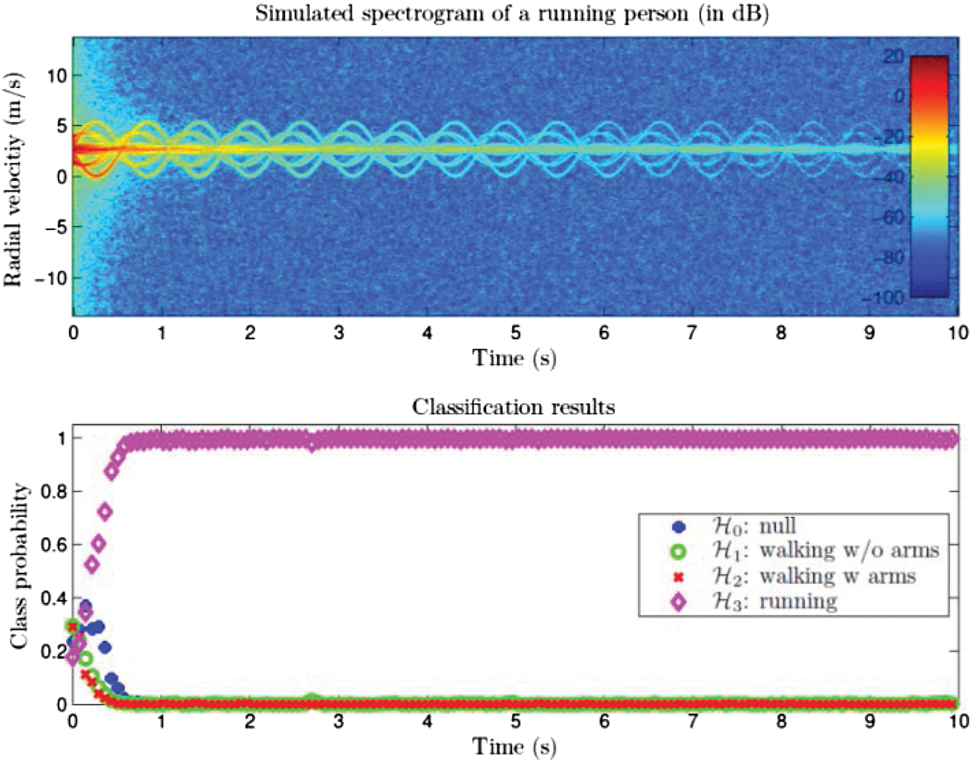
Fig. 5. Simulated spectrogram for a running human and its classification results.

B) Measured data

Measurements of humans (walking and running) and animals were performed in order to test the correct working of the algorithm on measured data. A schematic overview of the used measurement setup is depicted in Fig. 6. From this figure one can be note that the radar was positioned 0.5 m above the ground. Also, the target moves in a radial position away from the radar, starting from a known position. The radar used for the measurements is a continuous wave (CW)-radar which transmits a signal with a frequency of 24 GHz. The effective isotropic power of the transmit antenna was −10 dBW. The radar video signal is sampled with a sample frequency of 8820 Hz. After some post-processing (e.g. correcting the I-Q balance) the STFT is performed on the radar video signal in order to obtain the spectrogram. In the STFT a sliding window of 512 samples is used.

Fig. 6. Schematic overview of the measurement setup.

In the top part of Fig. 7, the measured spectrogram of a walking person is given. The walking person has a length of 1.85 m. Looking at the velocity of the torso, the average walking velocity can be extracted from the spectrogram and is assumed to be constant at 1.55 m/s. The bottom part of Fig. 7 shows the classification result. From this figure one can see that the part of the spectrogram, which contains the motion of the walking human (up to about 5.5 s), is classified correctly as human walking. When the person stops moving, the algorithm classifies this part also correctly as the null-hypothesis. The estimation results of the motion parameters at t = 5.18 s are given in Fig. 8. The results of the estimation of the motion parameters are indicated in Table 2.

Fig. 7. Measured spectrogram for a walking human and its classification results.

Fig. 8. Parameter estimation for measurement with a walking human.

Table 2. Parameter estimation results in a measurement performed for both a walking and a running person.

A similar test is performed with measurement of a running person. The spectrogram of this person is indicated in the top part of Fig. 9. In the first 0.5 s of the measurement, the person is accelerating toward running, and this part of the measurement is classified as the null-hypothesis. Between around 0.5 and 2.5 s, the motion of a running person can be visually noticed in the spectrogram. The algorithm classifies this part correctly, as is observed in the bottom part of Fig. 9. After 2.5 s the person is slowing down and no human motion is recognized by the algorithm. Estimated parameters at t = 2.21 are indicated in Table 2.

Fig. 9. Measured spectrogram for a running human and its classification results.

Last, to test whether the filter is classifying motion not originating from humans correctly, measurements on moving animals were performed. In Fig. 10, the spectrogram of a duck is depicted. Since a duck is bipedal like humans, a walking duck shows some similarities to human walking. Especially the peaks coming from the feet and the torso component are similar to human walking. On the other hand, a duck makes shorter and quicker steps, and therefore explains the more spike-like nature of the spectrogram.

Fig. 10. Measured spectrogram of a duck and its classification results.

After 4.5 s the duck stops moving and hence no motion occurs anymore. This allows the same spectrogram to be used for testing when no motion is classified correctly. In the bottom part of Fig. 10 the classification results are indicated. From this figure one can observe that both the movement of the duck and the part containing no motion are classified correctly.