2.1. Conventional federated filter architecture

A federated filter is a type of two level data fusion structure, which works in parallel in each sub-filter (Wang et al., Reference Wang, Liu, Xiong and Zhong2014; Hide and Hill, Reference Hide and Hill2007). As shown in Figure 1, it is a scheme comprising of a reset federated filter with a fault isolation module.

Figure 1. Scheme of reset federated filter with fault isolation module.

In the federated filter algorithm, each sub-system works independently to complete the Kalman filter calculation. The local estimation $\hat{\bi X}_{i}$ and the corresponding covariance matrix P_i are obtained. The global optimal estimation $\hat{\bi X}_{g}$ and the corresponding covariance matrix P_g are obtained by means of information fusion in the global filter. The calculation methods are shown as Equation (1). This process is called information fusion. At the same time, the values of $\hat{\bi X}_{g}$ and P_g are required to be fed back to each subsystem according to Equation (2). This process is called information sharing.

The fault detection modules monitor the fault state of the subsystem in real time to ensure that the fault information can be isolated when it occurs, in case of contamination of other normal subsystems through the process of information sharing.

The information fusion:

(1)$$\eqalign{ {\bi P}_g &= \left( {\sum\limits_{i = 1}^N {{\bi P}_i^{ - 1} } } \right)^{ - 1} \cr \hat{{\bi X}}_g &= {\bi P}_g\left( {\sum\limits_{i = 1}^N {{\bi P}_i^{ - 1} } {\hat{{\bi X}}}_i} \right)}$$

The information sharing:

(2)$$\eqalign{{\bi P}_i &= \beta _i^{ - 1} {\bi P}_g \cr \hat{{\bi X}}_i{\rm } &= \hat{{\bi X}}_g}$$

where $\sum\limits_{i=1}^{N} \beta_{i}=1$ (Qin, Reference Qin2012).

In the conventional reset federated filter, the sensor should be isolated immediately when the fault is detected, and the filter should be reconstructed by the fault free subsystems. However, some sensor faults cannot always be detected immediately, such as slowly-varying faults, which will cause a lasting impact on the stability and accuracy of the system.

2.2. Adaptive federated filter scheme

In order to overcome the shortcomings in the conventional reset federated filter algorithm, this paper proposes a dynamic vector-formed information sharing algorithm based on two-state chi square detection. The scheme is shown in Figure 2.

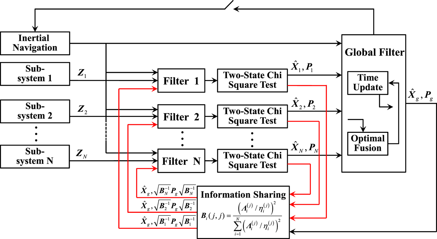
Figure 2. Scheme of vector-formed information sharing algorithm based on two-state chi square detection.

The Kalman filter is established based on the state equation and measurement equation of the navigation system. A two-state chi square detection function is designed to obtain the fault detection value of each state. Then the vector-formed information sharing coefficients of the federated filter (B_i) are calculated based on the fault detection value and the fault detection threshold. After that, the local estimation $\hat{\bi X}_{i}$ and corresponding covariance matrix P_i of each sub-filter are calculated according to the global optimal estimation $\hat{\bi X}_{g}$, covariance matrix P_g and the vector-formed information sharing coefficients B_i. In addition, as the vector-formed information sharing coefficients are obtained from the fault detection values, the adaptive adjustment of measurement noise can be achieved by using the relationship between the state and measurement information. Then the information distribution process is completed.

The method proposed in the paper removes the fault isolation module in the conventional reset federated filter, reduces the influence of fault information on the global estimation and improves the adaptability of the federated filter in the case of subsystem failure.

3.1. Model of a federated filter

3.1.1. State equation of the system

In the scheme designed in Figure 2, east-north-up coordinates are selected as the navigation coordinates and the system state is selected as follows.

$${\bi X} = [\varphi _E,\varphi _N,\varphi _U,\delta v_E,\delta v_N,\delta v_U,\delta L,\delta \lambda ,\delta h,\varepsilon _{bx},\varepsilon _{by},\varepsilon _{bz},\varepsilon _{rx},\varepsilon _{ry},\varepsilon _{rz},\nabla _x,\nabla _y,\nabla _z]^T$$

where φ_E, φ_N, φ_U are platform misalignment angles; δv _E, δv _N, δv _U are the velocity errors; δL, δλ, δh are the latitude, longitude and height errors; ε_bx, ε_by, ε_bz and ε_rx, ε_ry, ε_rz are the constant drift errors and the first order Markov drift errors of gyroscopes and $\nabla_{x}\comma \; \nabla _{y}\comma \; \nabla_{z}$ are the first order Markov drift errors of accelerometers. By the analysis of the strap-down inertial navigation system error source, the state equation is obtained as:

(3)$${\bi X}_k = {\bi \Phi }_{k \vert k - 1}{\bi X}_{k - 1} + {\bi G}_{k - 1}{\bi W}_{k - 1}$$

where Φ_k|k−1, G_k−1 and W_k−1 are the system matrix, white noise error matrix and white noise error vector of error equation of the inertial navigation system, respectively.

3.1.2. Measurement equation of the system

According to the output characteristics of each sensor subsystem, the linear measurement equation is established.

3.1.2.1. Measurement Equation of SINS/GPS (Li et al., Reference Li, Wang and Gao2016)

In SINS/GPS integrated navigation, GPS provides velocity and position information. The measurement equation is as follows:

(4)$$\eqalign{ {\bi Z}_{GPS,k} &= {\bi H}_{GPS,k}{\bi X}_k + {\bi V}_{GPS,k} \cr & = \left[ {\matrix{ {(L_I - L_G)R_M} \cr {(\lambda_I - \lambda_G)R_N\cos L} \cr {h_I - h_G} \cr {\upsilon_{IE} - \upsilon_{GE}} \cr {\upsilon_{IN} - \upsilon_{GN}} \cr {\upsilon_{IU} - \upsilon_{GU}} \cr } } \right] = \left[ {\matrix{ {R_M\delta L} \cr {R_N\cos L\delta \lambda } \cr {\delta h} \cr {\delta \upsilon_E} \cr {\delta \upsilon_N} \cr {\delta \upsilon_U} \cr } } \right] + \left[ {\matrix{ {w_{G1}} \cr {w_{G2}} \cr {w_{G3}} \cr {w_{G4}} \cr {w_{G5}} \cr {w_{G6}} \cr } } \right] \cr & = \left[ {\matrix{ {0_{3 \times 3}} & {0_{3 \times 3}} & {diag[\matrix{ {R_M} & {R_N\cos L} & 1 \cr } ]} & {0_{3 \times 9}} \cr {0_{3 \times 3}} & {diag[\matrix{ 1 & 1 & 1 \cr } ]} & {0_{3 \times 3}} & {0_{3 \times 9}} \cr } } \right]{\bi X}_k + \left[ {\matrix{ {w_{G1}} \cr {w_{G2}} \cr {w_{G3}} \cr {w_{G4}} \cr {w_{G5}} \cr {w_{G6}} \cr } } \right]}$$

where Z_GPS,k is the measurement information of the difference between SINS and GPS of the position and velocity at k time, H_GPS,k is the measurement coefficient matrix and V_GPS,k is the measurement noise of independent zero-mean Gaussian white-noise processes.

3.1.2.2. Measurement Equation of SINS/CNS (Wang et al., Reference Wang, Cui, Li and Ye2017)

In SINS/CNS integrated navigation, the CNS provides attitude information. The measurement equation is as follows:

(5)$$\eqalign{ {\bi Z}_{CNS,k} &= {\bi H}_{CNS,k}{\bi X}_k + {\bi V}_{CNS,k} \cr & = \left[ {\matrix{ {\gamma_I - \gamma_C} \cr {\theta_I - \theta_C} \cr {\psi_I - \psi_C} \cr } } \right] = \left[ {\matrix{ {{\bi A}_{3 \times 3}} & {0_{3 \times 15}} \cr } } \right]{\bi X}_k + \left[ {\matrix{ {w_{\gamma C}} \cr {w_{\theta C}} \cr {w_{\psi C}} \cr } } \right]}$$

where A_3×3 is the transformation matrix from INS platform error angle to attitude error angle, and:

$${\bi A}_{3 \times 3} = \displaystyle{{ - 1} \over {\cos \theta }}\left[ {\matrix{ {\sin \psi } & {\cos \psi } & 0 \cr {\cos \psi \cos \theta } & { - \sin \psi \cos \theta } & 0 \cr {\sin \psi \sin \theta } & {\cos \psi \sin \theta } & { - \cos \theta } \cr } } \right]$$

where θ and ψ are the value of the pitch and heading angle, respectively.

Z_CNS,k is the measurement information of the difference between SINS and CNS of the roll, pitch and heading angle at k time, H_CNS,k is the measurement coefficient matrix and V_CNS,k is the measurement noise of independent zero-mean Gaussian white-noise processes.

3.1.2.3. Measurement equation of SINS/SAR (Yang et al., Reference Yang, Peng, Zhang and Shan2010)

In SINS/SAR integrated navigation, SAR provides horizontal position information. The measurement equation is as follows:

(6)$$\eqalign{ {\bi Z}_{SAR,k} &= {\bi H}_{SAR,k}{\bi X}_k + {\bi V}_{SAR,k} \cr & = \left[ {\matrix{ {(L_I - L_S)R_M} \cr {(\lambda_I - \lambda_S)R_N\cos L} \cr } } \right] = \left[ {\matrix{ {0_{1 \times 6}} & {R_M} & 0 & {0_{1 \times 10}} \cr {0_{1 \times 6}} & 0 & {R_N\cos L} & {0_{1 \times 10}} \cr } } \right]{\bi X}_k + \left[ {\matrix{ {w_{1S}} \cr {w_{2S}} \cr } } \right]}$$

where Z_SAR,k is the measurement information of the difference between SINS and SAR of the latitude and longitude at k time, H_SAR,k is the measurement coefficient matrix and V_SAR,k is the measurement noise of independent zero-mean Gaussian white-noise processes.

In this paper, the three subsystems are used as examples to verify the correctness of the algorithm. For other sensors, the algorithm can also be applied.

3.1.3. Kalman filter of the sub-system

According to the system state equation and measurement equation established in Equations (3)–(6), the closed loop Kalman filter of sub-systems are designed as shown in Equation (7) (Zhong et al., Reference Zhong, Liu, Li and Wang2017):

(7)$$\eqalign{\hat{{\bi X}}_{i,k \vert k - 1} &= {\bi \Phi }_{k \vert k - 1}\hat{{\bi X}}_{i,k - 1 \vert k - 1} \cr {\bi P}_{i,k \vert k - 1} &= {\bi \Phi }_{k \vert k - 1}{\bi P}_{i,k - 1 \vert k - 1}{\bi \Phi }_{k \vert k - 1}^T + {\bi G}_{k - 1}{\bi Q}_{k - 1}{\bi G}_{k - 1}^T \cr {\bi P}_{i,k \vert k} &= ({\bi I} - {\bi K}_{i,k}{\bi H}_{i,k}){\bi P}_{i,k \vert k - 1}({\bi I} - {\bi K}_{i,k}{\bi H}_{i,k})^T + {\bi K}_{i,k}{\bi R}_{i,k}{\bi K}_{i,k}^T \cr {\bi K}_{i,k} &= {\bi P}_{i,k \vert k - 1}{\bi H}_{i,k}^T ({\bi H}_{i,k}{\bi P}_{i,k \vert k - 1}{\bi H}_{i,k}^T + {\bi R}_{i,k})^{ - 1} \cr \hat{{\bi X}}_{i,k \vert k} &= \hat{{\bi X}}_{i,k \vert k - 1} + {\bi K}_{i,k}\lpar {{\bi Z}_{i,k} - {\bi H}_{i,k}{\hat{{\bi X}}}_{i,k \vert k - 1}} \rpar }$$

After each sub-filter is finished to obtain the corrections, the information fusion is carried out according to Equation (1) to obtain the optimal estimate $\hat{\bi X}_{g}$.

3.2. Two-state chi square detection algorithm

In each Kalman filter sub-system, a two-state chi square detection function is designed to evaluate the quality of each state information. We define the state variable $\hat{\bi X}_{i\comma k\vert k}^{S}$ and the covariance matrix of state estimation ${\bi P}_{i\comma k\vert k}^S $:

(8)$$\eqalign{\hat{{\bi X}}_{i,k \vert k}^S &= {\bi \Phi }_{k \vert k - 1}\hat{{\bi X}}_{i,k - 1 \vert k - 1}^S \cr {\bi P}_{i,k \vert k}^S &= {\bi \Phi }_{k \vert k - 1}{\bi P}_{i,k - 1 \vert k - 1}^S {\bi \Phi }_{k \vert k - 1}^T + {\bi G}_{k - 1}{\bi Q}_{k - 1}{\bi G}_{k - 1}^T }$$

Define the state estimation errors $\tilde{\bi X}_{i\comma k}$ and $\tilde{\bi X}_{i\comma k}^{S}$:

(9)$$\eqalign{& \tilde{{\bi X}}_{i,k} = {\bi X}_k - \hat{{\bi X}}_{i,k \vert k} \cr & \tilde{{\bi X}}_{i,k}^S = {\bi X}_k - \hat{{\bi X}}_{i,k \vert k}^S }$$

Then the state difference δ e_i,k can be expressed as:

(10)$$\delta {\bi e}_{i,k} = \tilde{{\bi X}}_{i,k} - \tilde{{\bi X}}_{i,k}^S = \hat{{\bi X}}_{i,k \vert k}^S - \hat{{\bi X}}_{i,k \vert k}$$

$\hat{\bi X}_{i\comma k\vert k}^{S}$ is the state variable of the state propagator. $\hat{\bi X}_{i\comma k\vert k}$ is the state of the Kalman filter and it is assigned through the global state. So, we obtain the covariance matrix of state difference:

(11)$$\eqalign{{\bi T}_{i,k} &= E\{ \delta {\bi e}_{i,k}\delta {\bi e}_{i,k}^T \} \cr & = E\{ \tilde{{\bi X}}_{i,k}(\tilde{{\bi X}}_{i,k})^T + \tilde{{\bi X}}_{i,k}^S (\tilde{{\bi X}}_{i,k}^S )^T - \tilde{{\bi X}}_{i,k}(\tilde{{\bi X}}_{i,k}^S )^T - \tilde{{\bi X}}_{i,k}^S (\tilde{{\bi X}}_{i,k})^T\} \cr & = {\bi P}_{i,k \vert k} + {\bi P}_{i,k \vert k}^S - {\bi P}_{i,k \vert k}^{KS} - ({\bi P}_{i,k \vert k}^{KS} )^T}$$

If we let ${\bi P}_{i\comma 0\vert 0} ={\bi P}_{i\comma 0\vert 0}^{KS} $, we can obtain ${\bi P}_{i\comma k\vert k} ={\bi P}_{i\comma k\vert k}^{KS}$ (Qin, Reference Qin2012), then:

(12)$${\bi T}_{i,k} = {\bi P}_{i,k \vert k}^S - {\bi P}_{i,k \vert k}$$

Thus, we can get the fault detection function corresponding to each component in the state X_k:

(13)$$\eta _{i,k}^{(j)} = \displaystyle{{{(\delta {\bi e}_{i,k}^{(j)} )}^2} \over {{\bi T}_{i,k}(j, j)}},j = 1,2, \cdots ,18$$

where $\eta_{i\comma k}^{\lpar j\rpar }$ obeys χ²(1) chi square distribution (Da, Reference Da1994).

In the recursive process of Equation (8), ${\bi P}_{i\comma k\vert k}^S$ will deviate more and more greatly from the real value because of the influence of system noise and modelling error (Yang et al., Reference Yang, Zhang and Guo2016; Zhu et al., Reference Zhu, Cheng and Wang2016). Therefore, we design a two-state chi square detection method, whose structure is shown in Figure 3. The two states of the recursion work alternately, and they are periodically reset with P_i,k|k. We divide the whole time into t ₁ ∈ [2nT, (2n + 1) T), $t_{2} \in \lsqb \lpar 2n+1\rpar T\comma \; \ \lpar 2n+2\rpar T\rpar $ and t ₃ ∈ {nT}, where n ∈ {0, 1, 2, …} and T is the reset cycle for state recursion. The state recursions are set the same initial values. When t ∈ t ₁, state recursions A and B are recursive by their own processes, and the state chi square detection function is calculated by ${\bi P}_{i\comma k\vert k}^{SA}$. When t ∈ t ₂, state recursions A and B are recursive by their own processes respectively, and the state chi square detection function is calculated by ${\bi P}_{i\comma k\vert k}^{SB}$. When t ∈ t ₃ and n is an odd number, the state recursion A is reset, that is ${\bi P}_{i\comma k\vert k}^{SA} ={\bi P}_{i\comma k\vert k}$. When t ∈ t ₃ and n is an even number, the state recursion B is reset, that is ${\bi P}_{i\comma k\vert k}^{SB} ={\bi P}_{i\comma k\vert k}$. By resetting the state recursion, the divergence of ${\bi P}_{i\comma k\vert k}^{S}$ caused by the system error and modelling error can be avoided, as can an abnormal value of the fault detection function, so as to improve the accuracy of fault detection.

Figure 3. Scheme of two-state chi square detection.

3.3. Design of vector-formed information sharing coefficients

In Section 3.2, the fault detection value of each state ($\eta_{i\comma k}^{\lpar j\rpar }$) is calculated by using the two-state chi square detection algorithm. This reflects the quality of different states in each sub-system. According to the fault detection value of each subsystem states calculated in Equation (13), the vector-formed information sharing coefficients of each subsystem are designed as in Equation (14):

(14)$${\bi B}_{i,k}(j, j) = \displaystyle{{{({\bi \Lambda }_i^{(j)} /\eta _{i,k}^{(j)} )}^2} \over {\sum\nolimits_{i = 1}^N {{({\bi \Lambda }_i^{(j)} /\eta _{i,k}^{(j)} )}^2} }}$$

where ${\bi {\Lambda}}_{i}^{\lpar j\rpar }$ is the fault detection threshold chosen from the table of chi square distribution.

When the subsystem is working properly, then ${{\bi \Lambda}}_{i}^{\lpar j\rpar }/\eta_{i\comma k}^{\lpar j\rpar } >1$. If the subsystem fails, $\eta_{i\comma k}^{\lpar j\rpar }$ increases and exceeds the threshold, then $0< {\bi \Lambda}_{i}^{\lpar j\rpar } /\eta_{i\comma k}^{\lpar j\rpar } <1$. $\eta_{i\comma k}^{\lpar j\rpar }$ is the fault detecting value of the state. So, if the corresponding state fails more seriously, $\eta_{i\comma k}^{\lpar j\rpar }$ becomes larger, and then the ${\bi \Lambda}_{i}^{\lpar j\rpar } /\eta_{i\comma k}^{\lpar j\rpar }$ becomes smaller.

In Equation (14), the bigger $\eta_{i\comma k}^{\lpar j\rpar }$ is, the smaller the corresponding B_i,k(j, j). That is, the smaller the information value that is shared. Through this distribution method, this paper realises the adaptive adjustment for fault information and improves the robustness of the system. In addition, Equation (14) satisfies $\sum_{i=1}^{N} {\bi B}_{i\comma k}={\bi I}$, in line with the law of conservation of information in a federated filter.

The expressions of the federated filter vector-formed information sharing are shown as follows:

(15)$$\eqalign{{\bi P}_{i,k \vert k}^{ - 1} &= {\bi B}_{i,k}^{1/2} {\bi P}_g^{ - 1} {\bi B}_{i,k}^{1/2} \cr {\bi Q}_i^{ - 1} &= {\bi B}_{i,Q}^{1/2} {\bi Q}_g^{ - 1} {\bi B}_{i,Q}^{1/2} \cr \hat{{\bi X}}_{i,k \vert k} &= \hat{{\bi X}}_g}$$

where B_iQ is a diagonal matrix composed of the nine diagonal elements of B_i,k(10, 10) ~ B_i,k(18, 18), which corresponds to the system noise.

3.4. Adaptive adjustment of measurement noise

This section mainly describes the adaptive method of calculation of R_i,k in the Kalman filter equation. In the information sharing vector, the component does not correspond to the measurement information, so it needs to be converted. The following is a description of the conversion method, which is used to calculate the adaptive adjustment parameters.

3.4.1. Attitude measurement information conversion

The parameters used in the system state are the platform error angles $[\matrix{ {\varphi _E} & {\varphi _N} & {\varphi _U} \cr } {\rm ]}^T$, and the attitude error angles $[\matrix{ {\delta \gamma } & {\delta \theta } & {\delta \psi } \cr }]^T$ are used in the measurement information (δγ, δθ, and δ ψ represent the error of roll, pitch and heading, respectively). The conversion relation is shown as follows:

(16)$$\left[ {\matrix{ {\delta \gamma } \cr {\delta \theta } \cr {\delta \psi } \cr } } \right] = {\bi H}_\varphi \left[ {\matrix{ {\varphi_E} \cr {\varphi_N} \cr {\varphi_U} \cr } } \right]$$

where

$${\bi H}_\varphi = - \displaystyle{1 \over {\cos \theta }}\left[ {\matrix{ {\sin \psi } & {\cos \psi } & 0 \cr {\cos \psi \cos \theta } & { - \sin \psi \cos \theta } & 0 \cr {\sin \psi \sin \theta } & {\cos \psi \sin \theta } & { - \cos \theta } \cr } } \right]$$

Then the adjustment coefficients of attitude measurement noises are:

(17)$$\left[ {\matrix{ {b_{i,k}^1 } \cr {b_{i,k}^2 } \cr {b_{i,k}^3 } \cr } } \right] = {\bi H}_\varphi \left[ {\matrix{ {{\bi B}_{i,k}(1,1)} \cr {{\bi B}_{i,k}(2,2)} \cr {{\bi B}_{i,k}(3,3)} \cr } } \right]$$

After normalisation, we get:

(18)$${\bi B}_{i,k}^\varphi (j,j) = \displaystyle{{b_{i,k}^j } \over {\sum\limits_{i = 1}^N {b_{i,k}^j } }},\;j = 1,2,3$$

${\bi B}_{i\comma k}^{\varphi}$ is the adaptive parameter for the attitude measurement noise. The modified attitude measurement noise covariance matrix is:

(19)$${\bi R}_{i,k}^\varphi = \lpar {{\bi B}_{i,k}^\varphi } \rpar ^{ - 1}R_{i,0}^\varphi$$

where ${\bi R}_{i\comma 0}^{\varphi}$ is the initial attitude measurement noise covariance matrix.

3.4.2. Velocity measurement information conversion

In the velocity measurement information, the transformation matrix is:

$${\bi H}_v = \left[ {\matrix{ 1 & 0 & 0 \cr 0 & 1 & 0 \cr 0 & 0 & 1 \cr } } \right]$$

The states of the system correspond to the measurement information. So, we can obtain:

$${\bi B}_{i,k}^v = \left[ {\matrix{ {{\bi B}_{i,k}(4,4)} & 0 & 0 \cr 0 & {{\bi B}_{i,k}(5,5)} & 0 \cr 0 & 0 & {{\bi B}_{i,k}(6,6)} \cr } } \right]$$

${\bi B}_{i\comma k}^{v}$ is the adaptive parameter for the velocity measurement noise. The modified velocity measurement noise covariance matrix is:

(20)$${\bi R}_{i,k}^v = \lpar {{\bi B}_{i,k}^v } \rpar ^{ - 1}{\bi R}_{i,0}^v$$

where ${\bi R}_{i\comma 0}^{v}$ is the initial velocity measurement noise covariance matrix.

3.4.3. Position measurement information conversion

In the position measurement information, the transformation matrix is:

$${\bi H}_p = \left[ {\matrix{ {R_M} & 0 & 0 \cr 0 & {R_N\cos L} & 0 \cr 0 & 0 & 1 \cr } } \right]$$

where R _M and R _N are the radii of curvature of the principal vertical circle and prime vertical circle in the reference ellipsoid. L represents latitude.

The states of the system are corresponding to the measurement information. So, we can obtain:

$${\bi B}_{i,k}^p = \left[ {\matrix{ {{\bi B}_{i,k}(7,7)} & 0 & 0 \cr 0 & {{\bi B}_{i,k}(8,8)} & 0 \cr 0 & 0 & {{\bi B}_{i,k}(9,9)} \cr } } \right]$$

${\bi B}_{i\comma k}^{p}$ is the adaptive parameter for the position measurement noise. The modified position measurement noise covariance matrix is:

(21)$${\bi R}_{i,k}^p = \lpar {{\bi B}_{i,k}^p } \rpar ^{ - 1}{\bi R}_{i,0}^p$$

where ${\bi R}_{i\comma 0}^{p}$ is the initial position measurement noise covariance matrix.

4.1. Simulation description

The designed flight path is shown in Figure 4. The simulation time is 3,600 seconds and the initial position is 20° North latitude and 110° East longitude. The initial flight speed is zero and the heading is 090°.

Figure 4. The flight trajectory.

Suppose that the update frequency of the SINS is 50 Hz, the output frequency of aided navigation systems is 1 Hz, and the information fusion period is 1 second. The error parameters of the inertial navigation system are shown in Table 1 and the error parameters of the other navigation systems are shown in Table 2.

Table 1. Error parameters of the inertial navigation system.

Table 2. Error parameters of the other navigation systems.

In order to verify the fault tolerance performance of the algorithm, the faults of the step signal and ramp signal are added in the longitudinal direction of SAR respectively. Figures 5 and 6 are the error curves with hard and soft faults in the longitudinal direction. The hard fault starts at the 300th second, for a duration of 200 seconds. The magnitude of the step signal is 20 times the horizontal position error. The soft fault also occurs from the 300th second to the 500th second and the slope of the ramp signal is 0·2. From Figure 5 and Figure 6 the impact of fault information on the sensor error is obvious. By adding fault information to the sensor output, we can test whether the proposed method in this paper can eliminate the influence of faults and maintain navigation accuracy.

Figure 5. Longitude error with hard fault.

Figure 6. Longitude error with soft fault.

4.2. Simulation results and analysis

4.2.1. Simulation for the adaptive federated filter

According to the above simulation conditions, the fault isolation method of two-state chi square detection and the dynamic vector-formed information sharing algorithm are simulated. In the fault isolation method, the fault information is detected by the two-state chi square in real time. When the fault occurs, the corresponding sensor is isolated, and the federated filter architecture is reconstructed. The information sharing coefficients of sub-filters are evenly distributed and known as β = 1/N; N is the number of health sensors.

First, the validity of the proposed algorithm is tested under normal conditions. Figure 7 gives the position error contrast curve without fault and Figure 8 is the velocity error contrast curve without fault. We can see that the algorithm proposed in this paper can realise the data fusion of multi-sensor information and obtain stable navigation results.

Figure 7. Position error contrast curve without fault.

Figure 8. Velocity error contrast curve without fault.

Figure 9 shows the values of information sharing coefficients for the position component. Line 1, Line 2 and Line 3 denote the coefficients of CNS, GPS and SAR respectively in the vector-formed information sharing algorithm. The sharing coefficients for each state of the three sensors change over time, and their sum is 1. Line 4 denotes the information sharing coefficient of the fault isolation method, which always equals 1/3 in the absence of a fault.

Figure 9. Information sharing coefficients of position. This figure shows the comparison of the vector-formed information sharing coefficients and the fixed distribution coefficients. Line 1, Line 2 and Line 3 are calculated according to Equation (14). As the fault detection values of each state ($\eta_{i\comma k}^{\lpar j\rpar }$) are different, the coefficients change over time. Line 4 represents the fixed distribution coefficient of the conventional method. It is only related to the number of sensors and equals to 1/3 during the whole process.

According to the simulation conditions set in Section 4.1, this paper analyses these two methods under the conditions of hard and soft faults, respectively. The curves of the position error are contrasted in Figures 10 and 12 and the contrast curves of the velocity error are shown in Figures 11 and 13. From the figures, we can see that the two-state chi square detection algorithm can detect the sensor anomaly very well after adding the hard fault in longitude, so as to isolate the fault and ensure navigation precision. However, in the case of a soft fault, it is unable to detect the abnormity in time due to the slow change of the fault, which leads to the sub-filter using the error information. When the period of the failure is over, the impact will last for some time. On the other hand, the proposed dynamic vector-formed information sharing algorithm based on two-state chi square detection has good performance in both hard and soft faults. By adjusting the vector-formed information sharing coefficients and the measurement noises, the system maintains high navigation accuracy and improves the robustness.

Figure 10. Position error curves with hard fault.

Figure 11. Velocity error curves with hard fault.

Figure 12. Position error curves with soft fault.

Figure 13. Velocity error curves with soft fault.

The contrasts of the two methods in different situations are shown in Tables 3 and 4. From the statistical results shown in the tables, we can see that there is no obvious difference in the position error and velocity error between the two methods when adding a hard fault in longitude. However, in the case of a soft fault, the longitude error of the conventional fault isolation method is increased by an order of magnitude. The error of the east velocity is also larger than that of the method proposed in this paper.

Table 3. Comparison of position error.

Table 4. Comparison of velocity error.

In order to test the applicability of the algorithm proposed in this paper, the algorithm is simulated and verified under different flight trajectories and different sensor frequencies.

4.2.2. Different flight trajectories

The flight trajectory is shown in Figure 14. The simulation time is 3,600 seconds and the initial position is 20° north latitude and 110° east longitude.

Figure 14. The flight trajectory.

The faults of a step signal and a ramp signal are added in the latitudinal direction of GPS. The hard fault starts at the 1,400th second, with a duration of 300 seconds. The magnitude of the step signal is 20 times the horizontal position error. The soft fault occurs from the 1,400th second to the 1,700th second and the slope of the ramp signal is 0·2. The other conditions are the same as those in Section 4.1. Figures 15–20 are the simulation curves.

Figure 15. Position error contrast curve without fault.

Figure 16. Velocity error contrast curve without fault.

Figure 17. Position error curves with hard fault.

Figure 18. Velocity error curves with hard fault.

Figure 19. Position error curves with soft fault.

Figure 20. Velocity error curves with soft fault.

4.2.3. Different frequencies

In this section, we mainly test the applicability of the algorithm under different sensor output frequencies. Suppose that the update frequency of the SINS is 100 Hz, the output frequency of aided navigation systems is 2 Hz, and the information fusion period is 0.5 second. We use the flight path shown in Figure 4 and the other conditions are the same as those in Section 4.1. Figures 21–26 are the corresponding simulation curves.

Figure 21. Position error contrast curve without fault.

Figure 22. Velocity error contrast curve without fault.

Figure 23. Position error curves with hard fault.

Figure 24. Velocity error curves with hard fault.

Figure 25. Position error curves with soft fault.

Figure 26. Velocity error curves with soft fault.

From Figures 15–26, we can see that the algorithms proposed in this paper can be applied to different flight trajectories and sensor output frequencies. It can eliminate the influence of a sensor failure on the navigation system, ensure the positioning accuracy and improve the robustness of the system.