


1. Introduction
Modern advanced open rotor engines produce thrust using two contra-rotating, coaxial propellers and will have significantly better fuel efficiency than current generation turbofan engines (Parker & Lathoud Reference Parker and Lathoud2010). However, the propellers must be carefully designed to ensure that the noise levels are acceptable, particularly at take-off, where aircraft must comply with strict community noise regulations. The noise spectrum produced by an isolated modern open rotor at a condition representative of take-off consists of a broadband level, in addition to numerous tones (Kingan et al. Reference Kingan, Blandeau, Tester, Joseph and Parry2011). These tones include ‘rotor-alone’ tones which occur at integer multiples of the blade passing frequency of each propeller as well as ‘interaction’ tones produced by the interaction of the blades with the unsteady flow field from the adjacent propeller. The dominant source of the interaction tones on isolated modern ‘cropped’ contra-rotating open rotors is believed to be the periodic unsteady loading on the downstream propeller blades caused by their interaction with the viscous wakes from the upstream propeller (see Kingan et al. Reference Kingan, Ekoule, Parry and Britchford2014).
In order to design an open rotor which produces an acceptable level of noise, suitable methods for noise prediction are required. There are a number of such methods available and although computational fluid mechanics (CFD)/computational aeroacoustics (CAA) and hybrid CFD/analytical methods are now commonly used for open rotor noise predictions, analytical models are still well suited for preliminary design studies that investigate the effect of different parameters on rotor noise. This is because of the relatively short computational time required and the large range of calculations that are needed at the early design stage in addition to the absence of sufficient geometric or aerodynamic details for a higher fidelity calculation. Here, our goal is to use an analytic model to investigate the viscous wake interaction tone noise generation mechanism. The general approach is to first model the convection of the viscous wakes behind the upstream propeller. A variety of different models are available for this purpose; a number of examples are described in Parry (Reference Parry1988, Reference Parry1997) but those are, clearly, not exclusive. The velocity field at the downstream propeller location is then decomposed into a Fourier series and the response of (unsteady loading on) the downstream propeller blades is calculated using a standard blade response function such as those described by Quaglia et al. (Reference Quaglia, Léonard, Moreau and Roger2017), Adamczyk (Reference Adamczyk1974a,Reference Adamczykb) and Roger & Carazo (Reference Roger and Carazo2010). The acoustic radiation is then calculated, using, for example, Hanson's (Reference Hanson1985) frequency-domain formulae or, as in this paper, using a time-domain formula such as that presented by Najafi-Yazdi, Brés & Mongeau (Reference Najafi-Yazdi, Brés and Mongeau2011).
Recently, the authors have presented an asymptotic analysis of a frequency-domain analytical model for these viscous wake interaction tones (Kingan & Parry Reference Kingan and Parry2019a) which was an extension of similar methods applied to rotor-alone tones (Parry Reference Parry1995). It was shown that the analytic model could be expressed in terms of a surface integral over a propeller source annulus and that, for a ‘many-bladed contra-rotating propeller’ (with a large number of blades on both propellers) this surface integral could be accurately evaluated using asymptotic methods in which the principle contributions to the integral come from small regions of the surface around certain ‘critical points’. These critical points can be divided into two general types: interior stationary points or boundary critical points. A critical design was also considered for which a line of interior stationary points occurred on the source annulus. The asymptotic formulae suggest that tones for which the leading-order contribution is produced by a line of critical points will radiate more efficiently than tones where the leading-order contribution comes from an isolated interior stationary point which, in turn, will radiate more efficiently than tones where the leading-order contribution comes from boundary critical points. (Indeed, for acoustic tones with zero azimuthal mode order, the asymptotic approach showed that there could exist continuum rings and disks of interior critical points, with the latter radiating even more efficiently than a critical design.) The asymptotic analysis yielded simple algebraic formulae for the acoustic pressure for each tone which, nonetheless, predict accurately the dependence of these tones on the propeller geometry and operating condition as well as the observer location. These formulae are of practical use as they show clearly the effect of blade geometry and operating condition on the radiated noise field. An important parameter which defines the blade geometry and has a significant influence on the radiated noise is blade sweep which we define as the distance that a propeller blade mid-chord is swept backwards from the pitch-change axis in a helical direction parallel to the local flow direction (see figure 2 in § 2).
The authors published a subsequent paper (Kingan & Parry Reference Kingan and Parry2019b) in which the asymptotic formulae were used to investigate the effect of downstream propeller blade sweep on viscous wake interaction tones. In particular, the asymptotic formulae were exploited to design a swept downstream propeller blade which produces viscous wake interaction tones with low amplitudes. The formulae also demonstrated the clear link between the radiation efficiency of the tones and the trace velocity of the upstream propeller wakes along the leading edge of the downstream propeller blades. It was shown that if the trace velocity of the upstream propeller wakes along the leading edge of the downstream propeller blades are subsonic across the entire span of the blade, then tones have low radiated amplitudes and that further increases in sweep generally lead to significant further decreases in noise levels.
In addition, the authors (Parry & Kingan Reference Parry and Kingan2019) introduced the phrase ‘event line’ to represent the points on the surface that represented the locations of the interactions between the front wakes and the rear blade leading edges at a fixed point in time. The event line rotates at the same speed as the interaction tone of interest and its shape is curved to represent the azimuthal locations of the blade–wake interactions, although at a fixed point in time. In the general case, the interaction times actually vary along the radius, so the spatial locations are adjusted, using the rotation speed of the interaction, to produce an effective fixed-time locus of the interactions – which represents the event line. The ‘event line’ is an extension of Tyler & Sofrin's (Reference Tyler and Sofrin1962) concept of an ‘event’ – representing the interaction between a wake centreline and a blade leading edge at a fixed radius – to one of a continuous radially distributed event. (It is of particular importance here to note that the ‘event line’ is not, in general, straight.) All of the interior critical points – that dominated the far-field sound radiation – also lay on the ‘event line’ and satisfied two particular physical criteria. Firstly, the speed of the ‘event line’ – at a particular radial and azimuthal location – must be precisely sonic when resolved in the direction of the observer. Secondly, the ‘event line’ must be normal to a line drawn from it to the observer. (To be precise here, as the ‘event line’ can be both curved and twisted in general, we must use the tangent to the ‘event line’ as defined by the well-known Serret–Frenet formulae.) These two criteria had originally been derived, for the thickness noise radiated from a supersonic single-rotating propeller, in the time domain by Amiet (Reference Amiet1988) where there was no need for a formal ‘event line’ as the sources are automatically locked to the blades themselves.
The purpose of this paper is to further explore wake interaction noise, using an analytic time-domain approach, to achieve an alternative (and, perhaps, more natural) understanding of the underlying physical processes that both supports and extends that obtained in the frequency domain. In particular, we use the method to show the physical mechanisms by which downstream propeller sweep can be used to reduce radiated noise levels. We believe that such an approach is novel. Many methods for predicting contra-rotating propeller interaction tone noise have used frequency-domain sound radiation formulae. Examples of such analytic or hybrid analytic–numerical noise prediction methods are described in Hanson (Reference Hanson1985), Parry (Reference Parry1988), Whitfield, Mani & Gliebe (Reference Whitfield, Mani and Gliebe1990a,Reference Whitfield, Mani and Gliebeb), Carazo, Roger & Omais (Reference Carazo, Roger and Omais2011), Kingan et al. (Reference Kingan, Ekoule, Parry and Britchford2014), Zachariadis, Hall & Parry (Reference Zachariadis, Hall and Parry2011), Kingan & Sureshkumar (Reference Kingan and Sureshkumar2014), Grasso et al. (Reference Grasso, Christophe, Schram and Verstraete2014), Ekoule et al. (Reference Ekoule, McAlpine, Kingan, Sohoni and Parry2015, Reference Ekoule, McAlpine, Parry, Kingan and Sohoni2017), Quaglia et al. (Reference Quaglia, Moreau, Roger and Fernando2016, Reference Quaglia, Léonard, Moreau and Roger2017), Moreau & Roger (Reference Moreau and Roger2018) and Kingan & Parry (Reference Kingan and Parry2019a,Reference Kingan and Parryb). In addition to these, primarily numerical approaches which utilise a frequency-domain sound radiation formulation include the methods described by Peters & Spakovszky (Reference Peters and Spakovszky2010), Sharma & Chen (Reference Sharma and Chen2013) and Envia (Reference Envia2015). Studies that have used time-domain methods to predict the noise radiated from contra-rotating propellers have, to our knowledge, used exclusively numerical approaches to predict the flow field and blade response e.g. Stürmer & Yin (Reference Stürmer and Yin2009), Colin et al. (Reference Colin, Blanc, Caruelle, Barrois and Djordjevic2012a,Reference Colin, Caruelle, Node-Langlois, Omais and Parryb), Colin, Caruelle & Parry (Reference Colin, Caruelle and Parry2012), Soulat et al. (Reference Soulat, Kernemp, Sanjose, Moreau and Fernando2013, Reference Soulat, Kernemp, Sanjose, Moreau and Fernando2016) (who used both time-domain and frequency-domain methods to predict the radiated noise) and Falissard & Delattre (Reference Falissard and Delattre2014). For single-rotating propellers there has been some work in the time domain that has been purely analytical, including that of Hanson (Reference Hanson1976), Amiet (Reference Amiet1988), Chapman (Reference Chapman1988a,Reference Chapmanb) and Prentice (Reference Prentice1994).
This paper uses a ‘retarded time’ formulation due to Najafi-Yazdi et al. (Reference Najafi-Yazdi, Brés and Mongeau2011) which is an extension of Farassat's formulation 1 to include the effect of a uniform axial flow. This formulation contains an integral which becomes singular when the blade moves towards the observer at sonic speed and is thus a good choice for the subsonic propellers considered here. An alternative is the ‘collapsing sphere formulation’ (see Farassat & Brown Reference Farassat and Brown1977). The collapsing-sphere formulation recasts the radiation integral in terms of a double integral – the outer integral summing contributions over all possible source times and the inner integral summing contributions from each point on the propeller surface which contribute at each source time. The location of these points is calculated using the concept of a collapsing sphere: the collapsing sphere is centred on the observer and has a radius which decreases at the speed of sound. All acoustic signals emitted from the spatial and (source) temporal points at which the sphere intersects the propeller blades will arrive at the observer at the same (reception) time. Brentner & Farassat (Reference Brentner and Farassat2003) noted that the integrand in the collapsing sphere formulation becomes singular when the surface normal vector is parallel to the radiation vector pointing from the source location to the observer. The singularities which occur in both the retarded time and collapsing sphere formulations thus correspond to the criteria of Amiet (Reference Amiet1988) for significant acoustic radiation from a supersonic single-rotating propeller.
These descriptions show a connection between the sharp peaks discovered, in the time domain, by Amiet (Reference Amiet1988), the collapsing sphere approach of Farassat & Brown (Reference Farassat and Brown1977) and our work here – as will become clear in § 4 where we explore conditions under which the peaks in the waveform can become enhanced. There is also some connection to the event line description of Parry & Kingan (Reference Parry and Kingan2019), although that work was based on a frequency-domain approach. However, we point out that the present authors’ analyses are: firstly, related primarily to the determination, in advance, of the noise source space/times that dominate to the radiated sound field; and, secondly, derived for contra-rotating architectures for which one of the main issues is the determination a priori of the source locations (particularly in the frequency domain), which is straightforward for single-rotating propellers on which the sources are continuously ‘locked’ to the blades.
It is worth discussing briefly the way the paper is set out. We start with the models for the blade wakes, blade response and acoustic radiation that will form the complete basis of the analysis. The wakes are assumed to be two-dimensional and a suitable wake model is given in § 2.1. It is important that the blade response model is quasi three-dimensional in order to account for the effects of sweep on the rear blade; a suitable model, and the method of its implementation in the time domain, are discussed in § 2.2; the acoustic radiation is calculated using a time-domain formulation which is described in § 2.3.
For the detailed analysis, we begin in § 3 with a straight-blade configuration. In this case the wake interactions occur simultaneously (in terms of source time) along the blade span and the blade response for this particular case is discussed in § 3.1. In § 3.2 we study the acoustic pressure radiated from a single blade radius which is observed to contain a series of impulses related to each blade-wake interaction. We discuss the considerable differences in the pressure time history at the observer location – both in impulse amplitude and periodicity – dependent on whether the corresponding blade is moving towards or away from the observer (as the blade rotates). These differences are shown to be caused by the source directivity and a Doppler effect. In radar these differences in the Doppler effect around the source region are referred to as micro Doppler effects (see, for example, Van Bladel Reference Van Bladel1976; Chen et al. Reference Chen, Li, Ho and Wechsler2006; Chen Reference Chen2019) and can occur either in a source region with both an advancing and a receding side, or in a source with non-uniform vibrational characteristics. However, there is little in the literature on the subject as it relates to turbofan or propeller noise. There is some evidence of these micro Doppler effects in the paper on pylon–propeller interaction by Ricouard et al. (Reference Ricouard, Julliard, Omais, Regnier, Parry and Baralon2010) in which the radiated noise was observed to be dependent on whether the propeller was travelling towards or away from the observer as it passed the pylon. In § 3.2 we also discuss the formulation of the acoustic pressure from each radius which, we show, is a product of a source strength-type term (which, in the time domain, is a source time derivative of the local unsteady loading) and a radiation efficiency-type term with all the micro Doppler effects being included solely in the latter. The radiated sound is discussed in terms of the contributions from each chord-wise location and the domination of the acoustic sources close to the leading edge. In § 3.3 we consider the sound from the complete blade span making use of the results from §§ 3.1 and 3.2. It is shown that although the blade-wake interactions occur simultaneously (in source time), because of the different propagation path lengths from sources at different radii, pressure impulses emitted from different radii can interfere constructively, in certain situations, such that the entire spanwise sound fields coalesce and produce particularly high-amplitude impulses or, alternatively, the spanwise sound fields can interfere (partially) destructively producing significant reductions in the radiated noise. Examples of these interference effects are shown and discussed in detail.
In § 4 we consider the more general case of a rear blade with a swept leading edge. We discuss how sweep can be used to ‘de-phase’ wake–blade interactions and how these can also be used to ‘de-phase’ the associated wake–blade interaction noise at an observer location. In addition we discuss the role of the trace Mach number, of the wake interaction along the downstream blade leading edge, in determining the magnitude of the radiated noise. Results are shown and discussed in detail.
The objective of this paper is to understand the effects of sweep on the sound radiated from the downstream propeller in the time domain. This physical understanding of the source generation and propagation processes can be obtained primarily from the analysis of the sound radiated from a single blade on the downstream propeller. The extension to calculate and analyse the total radiated sound field from all blades on the downstream propeller is straightforward, but is quite laborious and is well beyond the scope of the current paper, as it is then necessary to include the rather complicated interference effects that occur between the individual sound fields that are radiated from each of the downstream propeller blades and that interference warrants its own detailed investigation as it is of interest in its own right. Such analysis and discussion will thus be given elsewhere.
2. Formulation
In this section an analytical model, based on that described in Kingan & Parry (Reference Kingan and Parry2019a,Reference Kingan and Parryb) is presented for calculating the noise produced by the unsteady loading on the downstream blades due to their interaction with the mean velocity deficit caused by the viscous wakes of the upstream propeller. The situation is shown in figure 1. The propellers are immersed in a uniform airflow with Mach number  $M_x$ in the negative x-direction relative to the engine and the air has ambient density
  $\rho _0$ and speed of sound
  $c_0$. The upstream and downstream propellers rotate in the negative and positive
  $\phi $-directions at rotational speeds
  $\varOmega _1$ and
  $\varOmega _2$, respectively. The pitch-change axis of the reference blades on the front and rear propellers are located at
  $\phi = 0$ at time
  $\tau = 0$ and are separated by a distance g in the axial direction. Also note that the convention adopted in this paper will be that the subscripts 1 and 2 respectively denote parameters associated with the upstream and downstream propellers. The blades of both rotors have chord
  $c(r)$, mid-chord sweep
  $s(r)$ and sectional drag coefficient
  $C_D(r)$ and both rotors have B blades and the downstream rotor has diameter D, tip radius
  $R_t = D/2$ and hub radius
  $R_h$.

Figure 1. Advanced open rotor blades and coordinates.
2.1. Wake modelling
The unsteady loading on the downstream propeller blades at radius, r, is calculated using an equivalent two-dimensional problem in which the wakes from an upstream cascade of blades interact with the blades of a downstream cascade. This situation is illustrated in figure 2. The upstream and downstream blades translate vertically downwards and upwards at Mach numbers  $\varOmega _1r/c_0$ and
  $\varOmega _2r/c_0$, respectively. At time
  $\tau = 0$ the pitch-change axis of the front rotor reference blade is aligned with the pitch-change axis of the rear rotor reference blade at
  $y = 0$ and the vertical spacing between the mid-chord positions of the blades on each cascade is equal to
  $2{\rm \pi} r/B$. The blades are modelled as infinitely thin flat plates which are aligned with the local flow direction but otherwise have identical characteristics (chord length, sweep, lean and drag coefficient) to the actual rotor blade at that particular radius. Also, the effect of the flow induced by the rotors is neglected such that the stagger angle,
  $\alpha $, of each blade is defined by
  $\tan \alpha = zM_T/M_x$, where
  $z = 2r/D$ and
  $M_T = \varOmega D/2c_0$. The Mach number of the blades relative to the air flow is
  $M_r = \sqrt {M_x^2 + z^2M_T^2 } $ with corresponding relative velocity
  $U_r = M_rc_0$.

Figure 2. Schematic of the equivalent two-dimensional cascade problem (a). Sweep definition and velocity triangle (b).
The reference blade of the upstream cascade produces a wake with mean deficit velocity  ${\bar{u}}^{\prime}$ aligned with the negative
  $X_1$-direction (the chordwise direction – see figure 2) which will be modelled using the two-dimensional Gaussian model defined in Parry (Reference Parry1988, Reference Parry1997):
 \begin{equation}{\bar{u}}^{\prime}(r,Y_1) = 2U_{r_1}\sqrt {\displaystyle{{\ln 2} \over {\rm \pi}}} \sqrt {\displaystyle{{c_1C_{D_1}} \over {L_1}}} \; \exp \left\{ {-\displaystyle{{\ln 2} \over {b_{1/2}^2 }}Y_1^2 } \right\},\end{equation}
where  $Y_1$ is the chord-normal coordinate of the upstream rotor blade,
  $L_1 = [gM_{r_1}/M_x-s_1 + s_LM_{r_1}/M_{r_2}]$ is the length (or convection distance) of the wake which is defined as the distance along the helical path which the upstream blades trace through the air measured from the mid-chord of the upstream reference blade to the axial location of the leading edge of the downstream propeller blades,
  $s_L = s_2-c_2/2$ is the leading-edge sweep of the downstream propeller blade (see figure 2) and
  $b_{1/2}$ is the wake half-width which is defined as
  $b_{1/2} = {\textstyle{1 \over 4}}\sqrt {C_{D_1}c_1L_1} $.
Because the upstream blades are identical and evenly spaced, the periodic velocity deficit of the upstream cascade of blades in the unwrapped cascade representation is given by
 \begin{equation}{\bar{v}}^{\prime} = \mathop \sum \limits_{n = {-}\infty }^\infty {\bar{u}}^{\prime}\left( {r,Y_1 + \displaystyle{{2{\rm \pi} r\cos \alpha_1} \over {B_1}}} \right).\end{equation}
Because  ${\bar{v}}^{\prime}$ is periodic in
  $Y_1$, Poisson's summation formula can be used to convert this expression to a sum of convected harmonic gusts:
 \begin{equation}{\bar{v}}^{\prime} = \displaystyle{{B_1U_{r_1}C_{D_1}c_1G_{n_1}} \over {4{\rm \pi} r\cos \alpha _1}}\mathop \sum \limits_{n = {-}\infty }^\infty \exp \left\{ {{\rm i}\displaystyle{{nB_1} \over {r\cos \alpha_1}}Y_1} \right\},\end{equation}
where
 \begin{equation}G_{n_1} = \exp \left\{ {-{\left[ {\displaystyle{{n_1B_1b_{1/2}M_{r_1}} \over {zDM_x\sqrt {\ln 2} }}} \right]}^2} \right\}.\end{equation}
In order to calculate the unsteady loading on the downstream blade row, the velocity deficit incident on the chord line of the reference blade on the downstream cascade should be expressed in terms of the chordwise coordinate of that blade  $X_2$ (shown in figure 2). The
  $X_2$ coordinate is related to the
  $Y_1$ coordinate by the following expression:
 \begin{equation}Y_1 = (\varOmega _1 + \varOmega _2)r\tau \cos \alpha _1-g\sin \alpha _1-(X_2 + s_L)\sin (\alpha _1 + \alpha _2).\end{equation}
The upstream rotor wake deficit velocity is aligned with the  ${-}X_1$ coordinate and therefore the mean upwash velocity (which is the component of velocity in the
  $Y_2$ direction) onto the downstream reference blade is given by
  $w = {-}\sin (\alpha _1 + \alpha _2){\bar{v}}^{\prime}$. Substituting (2.5) into (2.4) yields
 \begin{equation}w = \mathop \sum \limits_{n_1 = {-}\infty }^\infty w_{n_1}\exp \{ {\rm i}k_X(U_{r_2}\tau -X_2)\} ,\end{equation}
where
 \begin{equation}w_{n_1} = {-}\; \displaystyle{{B_1C_{D_1}c_1U_{r_1}(M_{T_1} + M_{T_2})G_{n_1}} \over {2{\rm \pi} DM_{r_2}}}\exp \left\{ {-{\rm i}k_Xs_L-{\rm i}n_1B_1\displaystyle{{2g} \over D}\displaystyle{{M_{T_1}} \over {M_x}}} \right\},\end{equation}
and
 \begin{equation}k_X = \displaystyle{{2n_1B_1} \over {DM_{r_2}}}(M_{T_1} + M_{T_2}).\end{equation}
As mentioned above, the approach adopted here assumes that the convection of the wakes from the upstream propeller is not affected by the swirl and induced axial and radial velocity between the propellers. Clearly, the wakes produced by a practical propeller will in fact deform due to the induced velocities. It is, however, not our intention to address these additional wake deformation effects in this paper. Rather, the purpose of this paper is to present a framework for analysing the noise generated by blade-wake interactions and to show how the geometry of the downstream blades can be used to alter the timing of the blade-wake interactions at different radii and thus the level of noise which is produced. It is also important to note that, from an aerodynamic point of view, our approach follows the helicoidal surface theory of Hanson (Reference Hanson1980, Reference Hanson1983, Reference Hanson1985) in which the effects of induced flow – both axial and circumferential – are neglected. That approach has been shown to produce good agreement with measured data (see, for example, Parry & Crighton Reference Parry and Crighton1989; Parry Reference Parry1997). The effects of induced velocity are straightforward to include and methods similar to the one presented here, but which include these effects, have been validated against experimental and numerical data in Kingan et al. (Reference Kingan, Ekoule, Parry and Britchford2014) and Ekoule et al. (Reference Ekoule, McAlpine, Parry, Kingan and Sohoni2017).
2.2. Unsteady loading
The total unsteady lift force per unit area acting on the chord line of the reference blade can be expressed as the sum of the unsteady ‘responses’ of the blade to each upwash harmonic, i.e.
 \begin{equation}\Delta p = \mathop \sum \limits_{n_1 = 1}^\infty 2\; \Re \{ \Delta p_{n_1}\} ,\end{equation}
where  ${{\rm \Delta} }p_{n_1}$ is the response of the reference blade to a harmonic gust of the form
  $w_{n_1}\exp \{ {\rm i}k_X(U_{r_2}\tau -X_2)\} $ which is given by
 \begin{equation}\Delta p_{n_1} = 2{\rm \pi} \rho _0U_{r_2}w_{n_1}{\mathbb S}(\sigma _2,M_{r_2},\bar{X}_2,\varLambda )\exp \left\{ {{\rm i}2{\rm \pi} n_1\displaystyle{\tau \over T}} \right\},\; \end{equation}
where  $T = 2{\rm \pi} /[B_1(\varOmega _1 + \varOmega _2)]$ is the period of the loading,
  $\bar{X}_2 = 2X_2/c_2$ is a dimensionless chordwise coordinate,
  $\sigma _2 = k_Xc_2/2$ is the reduced frequency and
  ${\mathbb S}$ is a non-dimensional response function. In this paper we follow the approach used in Kingan & Parry (Reference Kingan and Parry2019a) and use the high-frequency response function of Adamcyzk (Reference Adamczyk1974a,Reference Adamczykb). In this approach it is assumed that the response of the reference blade to a gust of the form
  $w_{n_1}\exp \{ {\rm i}k_X(U_{r_2}\tau -X_2)\} $ is equal to that of a two-dimensional, semi-infinite flat plate immersed in a flow of velocity
  $U_{r_2}$ with a leading-edge sweep angle set such that the spanwise trace velocity of each gust along the leading edge is equal to the spanwise trace velocity of the wake centreline along the leading edge of the reference blade of the rotor. The equivalent problem is shown in figure 3. Because the gust convects with the flow, the spanwise (
 $Z_2$) component of the trace Mach number of the gust along the leading edge is given by
  $M_{r_2}\cot \varLambda $.

Figure 3. Swept flat-plate coordinate definitions.
At radius r, the time  $\tau = \tau _0(r) \gt 0$ at which the wake centreline from the reference blade on the upstream cascade, defined by
  $Y_1 = 0$, first impinges on the leading edge of the downstream reference blade, located at
  $X_2 = 0$, can be determined by setting
  $X_2 = Y_1 = 0$ in (2.5) and rearranging to yield
 \begin{equation}\tau _0(r) = \displaystyle{1 \over {c_0}}\left[ {\displaystyle{{gM_{T_1}} \over {M_x(M_{T_1} + M_{T_2})}} + S_L(r)} \right]\; ,\end{equation}
where, for convenience, we have introduced  $S_L(r) = s_L/M_{r_2}$. The spanwise trace Mach number of this impingement point can be evaluated by taking the derivative of
  $\tau _0(r)$ with respect to r, rearranging and making use of the inverse function theorem to yield
 \begin{equation}M_t = \displaystyle{1 \over {c_0}}\displaystyle{{{\rm d}r} \over {{\rm d}\tau _0}} = \displaystyle{1 \over {S^{\prime}_L}}.\end{equation}
The blade leading-edge sweep angle in the equivalent flat-plate response problem,  $\varLambda $, is set such that
  $M_t = M_{r_2}\cot \varLambda $ and thus
 \begin{equation}\tan \varLambda = M_{r_2}{S}^{\prime}_L.\end{equation}
Kingan & Parry (Reference Kingan and Parry2019a) express Adamczyk's high-frequency, isolated aerofoil response function in the following forms:
 \begin{equation}{\mathbb S}(\sigma _2,M_{r_2},\bar{X}_2,\varLambda ) = \displaystyle{{\exp \left\{ {-{\rm i}{\rm \pi} /4 + {\rm i}\sigma_2\displaystyle{{\left[ {(M_{r_2}^2 -{\tan }^2\varLambda )-\sqrt {M_{r_2}^2 -{\tan }^2\varLambda } } \right]} \over {[1-(M_{r_2}^2 -{\tan }^2\varLambda )]}}{\bar{X}}_2} \right\}} \over {{\rm \pi} \sqrt {{\rm \pi} \sigma _2{\bar{X}}_2} \sqrt {1 + \sqrt {M_{r_2}^2 -{\tan }^2\varLambda } } }}\; ,\; \end{equation}
for  $M_t \gt 1\; $ (so-called super-critical gusts), and
 \begin{align} {\mathbb S}(\sigma
_2,M_{r_2},{\bar{X}}_2,\varLambda )& = \exp \left\{ {-{\rm
i}\displaystyle{{\rm \pi} \over 4} + \displaystyle{{\rm i} \over
2}{\tan }^{{-}1}\sqrt {{\tan }^2\varLambda -M_{r_2}^2 } }
\right\} \cr &\quad \times \displaystyle{{\exp \left\{
{\sigma_2\displaystyle{{\left[ {-{\rm i}({\tan
}^2\varLambda -M_{r_2}^2 )-\sqrt {{\tan }^2\varLambda
-M_{r_2}^2 } } \right]} \over {(1 + {\tan }^2\varLambda
-M_{r_2}^2 )}}{\bar{X}}_2} \right\}} \over {{\rm \pi} \sqrt {{\rm \pi}
\sigma _2{\bar{X}}_2} {[1 + ({\tan }^2\varLambda -M_{r_2}^2
)]}^{1/4}}}\; , \end{align}
\begin{align} {\mathbb S}(\sigma
_2,M_{r_2},{\bar{X}}_2,\varLambda )& = \exp \left\{ {-{\rm
i}\displaystyle{{\rm \pi} \over 4} + \displaystyle{{\rm i} \over
2}{\tan }^{{-}1}\sqrt {{\tan }^2\varLambda -M_{r_2}^2 } }
\right\} \cr &\quad \times \displaystyle{{\exp \left\{
{\sigma_2\displaystyle{{\left[ {-{\rm i}({\tan
}^2\varLambda -M_{r_2}^2 )-\sqrt {{\tan }^2\varLambda
-M_{r_2}^2 } } \right]} \over {(1 + {\tan }^2\varLambda
-M_{r_2}^2 )}}{\bar{X}}_2} \right\}} \over {{\rm \pi} \sqrt {{\rm \pi}
\sigma _2{\bar{X}}_2} {[1 + ({\tan }^2\varLambda -M_{r_2}^2
)]}^{1/4}}}\; , \end{align}
for  $M_t \lt 1$ (so-called sub-critical gusts).
The accuracy of this response function in relation to the problem considered here is discussed in detail in appendix A of Kingan & Parry (Reference Kingan and Parry2019b). That paper considered a set of almost identical contra-rotating propellers to those considered here (the only significant difference being the blade numbers and a slight change in the tip Mach numbers). It was shown that the effect of including a correction to enforce the unsteady Kutta condition at the trailing edge had a negligible effect on the total unsteady loading on the propeller blade. Nevertheless, it is acknowledged that the response function used here is approximate and will not model the pressure jump on the blade surface close to the trailing edge accurately. This fact should be borne in mind when interpreting results presented later in the paper which depend on (2.15) for the chordwise distribution of loading (namely figures 6 and 8). Kingan & Parry (Reference Kingan and Parry2019b), following the analysis of Amiet (Reference Amiet1976), also showed that the high-frequency response function was expected to produce inaccurate results when the dimensionless parameter  $|\kappa |\lt {\rm \pi}/4$, where
 \begin{equation}\kappa \equiv \displaystyle{{\sigma _2\cos \varLambda \sqrt {M_{r_2}^2 {\cos }^2\varLambda -{\sin }^2\varLambda } } \over {(1-M_{r_2}^2 {\cos }^2\varLambda )}}.\end{equation}
This criterion is only satisfied in the examples presented in this paper for the case presented in figure 15, for which the gust trace velocity is sonic across the blade leading edge.
The effect of the spanwise trace Mach number on the sound field radiated from the leading edge of an aerofoil due to its interaction with a convected harmonic gust is well known. This phenomenon has been studied extensively in the context of sound radiated from the leading edge of an aerofoil immersed in a turbulent flow. For example, Amiet (Reference Amiet1975) presented formulae for calculating the sound radiated from a flat-plate aerofoil with infinite span. In this case, the radiated sound field only depends on gusts with supersonic wavenumbers. However, Amiet noted that the surface pressure spectrum on the aerofoil is dependent on both the sub- and supercritical gusts. Later studies, for example by Roger & Serafini (Reference Roger and Serafini2005) and Roger & Moreau (Reference Roger and Moreau2010), have extended Amiet's work to include the effect of finite span and the contribution of the subcritical gusts. Note, however, that all of these papers addressed interactions on non-rotating aerofoils.
2.3. Acoustic radiation
The far-field acoustic pressure at location  $\boldsymbol{x}$ and time t produced by a thin rotating blade immersed in a flow can be calculated using a slightly modified form of (3.19) in Najafi-Yazdi et al. (Reference Najafi-Yazdi, Brés and Mongeau2011):
 \begin{equation}p(\boldsymbol{x},t)\cong \displaystyle{1 \over {4{\rm \pi} c_0}}\displaystyle{\partial \over {\partial t}}\int_{R_h}^{R_t} {\int_0^{c_2} {\left[ {\displaystyle{{{{\rm \Delta} }p(X_2,r,\tau )\tilde{\boldsymbol{R}}\boldsymbol{\cdot }\boldsymbol{n}} \over {R^\ast (1-\boldsymbol{M}\boldsymbol{\cdot }\tilde{\boldsymbol{R}})}}} \right]} } _{\tau = t-R/c_0}{\rm d}X_2{\rm d}r.\end{equation}
This model assumes that the observer and rotating blade are immersed in a flow of Mach number  $M_x$ in the negative
  $x_1$ direction where
  $R = [R^\ast{ + } M_x(x_1-y_1)]/\; (1-M_x^2 )$ is described by Najafi-Yazdi et al. as the acoustic distance between the source and receiver positions,
  $R^\ast{ = } \sqrt {{(x_1-y_1)}^2 + (1-M_x^2 )[{(x_2-y_2)}^2 + {(x_3-y_3)}^2]} $ and the radiation vector
  $\tilde{\boldsymbol{R}} = \tilde{R}_1\boldsymbol{e}_1 + \tilde{R}_2\boldsymbol{e}_2 + \tilde{R}_3\boldsymbol{e}_3$, where
 \begin{equation}\tilde{R}_1 = \displaystyle{{(x_1-y_1) + M_xR^\ast } \over {R^\ast (1-M_x^2 )}},\quad \tilde{R}_2 = \displaystyle{{(x_2-y_2)} \over {R^\ast }},\quad \tilde{R}_3 = \displaystyle{{(x_3-y_3)} \over {R^\ast }},\end{equation}
and  $\boldsymbol{e}_1$,
  $\boldsymbol{e}_2$ and
  $\boldsymbol{e}_3$ represent unit vectors in the
  $x_1$,
  $x_2$ and
  $x_3$ directions, respectively. The source position is defined in Cartesian coordinates as
 \begin{equation}y_1 = {-}\displaystyle{{M_x} \over {M_{r_2}}}(s_L + X_2),\quad y_2 = r\cos \varPhi ,\quad y_3 = r\sin \varPhi ,\end{equation}
where  $\varPhi = \varOmega \tau -(2M_{T_2}/DM_{r_2})(s_L + X_2)$.
The receiver positions are defined in Cartesian coordinates as  $x_1 = R_r\cos \theta _r$,
  $x_2 = R_r\sin \theta _r\cos \phi $, and
  $x_3 = R_r\sin \theta _r\sin \phi $, where
  $R_r$ is the reception distance,
  $\theta _r$ is the reception polar angle and
  $\phi $ is the azimuthal angle of the observer.
The unit vector aligned with the local force exerted by the blade on the fluid is defined as
 \begin{equation}\boldsymbol{n} = {-}\displaystyle{{zM_{T_2}} \over {M_{r_2}}}\boldsymbol{e}_1-\displaystyle{{M_x} \over {M_{r_2}}}\sin \varPhi \boldsymbol{e}_2 + \displaystyle{{M_x} \over {M_{r_2}}}\cos {\Phi }\boldsymbol{e}_3,\end{equation}
and the Mach number of the source is defined as
 \begin{equation}\boldsymbol{M} = {-}\boldsymbol{e}_2zM_{T_2}\sin \varPhi + \boldsymbol{e}_3zM_{T_2}\cos \varPhi .\end{equation}
Each of the terms in the square brackets within the integrand in (2.17) is evaluated at the source (or retarded) time  $\tau = t-R/c_0$.
In this paper, we will also make use of ‘emission coordinates’ to define the position of the observer. These emission coordinates, defined by the radiation distance  $R_e$ and polar angle
  $\theta _e$, are related to the ‘reception coordinates’ via
  $R_r\cos \theta _r = R_e(\cos \theta _e-M_x)$ and
  $R_r\sin \theta _r = R_e\sin \theta _e$. In particular, the ‘emission radius’,
  $R_e$, is equal to the ‘radiation distance’, R, for a source located at the origin of the coordinate system at the ‘emission time’ (the time at which sound is emitted). The ‘emission polar angle’,
  $\theta _e$, is equal to the angle between the radiation vector,
  $\tilde{\boldsymbol{R}}$, and the
  $x$-axis and corresponds to the polar angle at which a ‘ray’, emitted from the origin and travelling at sonic velocity relative to the fluid, will reach the observer position.
3. Sound radiation from a straight blade
The propeller designs considered in this paper are representative of a modern advanced open rotor and are similar to those considered in Whitfield et al. (Reference Whitfield, Mani and Gliebe1990a,Reference Whitfield, Mani and Gliebeb) and have the following parameters:  $B_1 = 10$,
  $M_x = 0.1998$,
  $M_{T_1} = 0.70$,
  $M_{T_2} = 0.70$,
  $D = 0.6096\;{\rm m}$;
  $R_h = 0.2D$,
  $g = 0.2394D$,
  $C_{D_1} = 0.02$,
  $c_1 = c_2 = 0.1D$,
  $s_1 = 0$. The ambient speed of sound and density are
  $c_0 = 344.4\;{\rm m}\,{\rm s}^{{-}1}$ and
  $\rho _0 = 1.1192\;{\rm kg}\,{\rm m}^{{-}3}$. Here, as we argued in § 1, we will only consider the acoustic signature produced by one downstream blade. The method can be extended to study the acoustic interference effects that occur in radiation from multiple blades, but such analysis is rather complicated and beyond the scope of this paper. The upstream rotor blades have arbitrary sweep and no lean, whilst the downstream blade has arbitrary leading-edge sweep and no lean. Without any loss of generality, the observer is located in the acoustic far field at
  $R_e = 1000\;{\rm m}$,
  $\theta _e = {\rm \pi}/2$ radians and
  $\phi = \varOmega _2\tau _0(R_h)-{\rm \pi} /2$ radians. This ensures that the observer is located at an azimuthal angle
  $-{\rm \pi} /2$ radians from the azimuthal angle at which the centreline of the wake from the reference blade impinges on the leading edge of the downstream blade at the hub. At this time the blade is moving away from the observer location because, in our coordinate system, the blade rotates in the positive azimuthal (
 $\phi $) direction. Figure 4 shows a blade with zero leading-edge sweep (
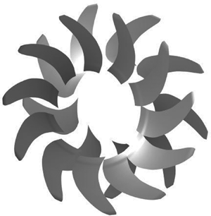
 $s_L = 0$ along the blade span) and the location of the wake centrelines (the blue radial lines) at the axial position of the blade leading edge at the instant the reference blade wake centreline impinges on the blade leading edge at the hub. In the figure, the view is along the propeller axis of rotation from an upstream location and the figure is rotated such that the observer (located in the acoustic far field) lies in the horizontal plane which contains the propeller axis.

Figure 4. Schematic showing a blade with zero leading-edge sweep, the location of the wake centrelines at the axial position of the blade leading edge and the observer position at source time  $\tau = \tau _0$.
It is important to check the validity of the numerical implementation of the time-domain method, even though the radiation formula of Najafi-Yazdi et al. (Reference Najafi-Yazdi, Brés and Mongeau2011) – on which our analysis is based – is well known. For this validation process we have compared the pressure time histories in the far field using both the method described in § 2.3 above and the frequency-domain method described by Hanson (Reference Hanson1985) and Parry (Reference Parry1988) and utilised by Kingan & Parry (Reference Kingan and Parry2019a) in their high blade number asymptotic approach. The frequency-domain method has been not only well documented but also well validated and well used in comparisons against model and even full-scale flight data (see Bradley Reference Bradley1986; Parry Reference Parry1988, Reference Parry1997; Parry & Crighton Reference Parry and Crighton1989; Hoff Reference Hoff1990; Kingan et al. Reference Kingan, Ekoule, Parry and Britchford2014; Ekoule et al. Reference Ekoule, McAlpine, Parry, Kingan and Sohoni2017). Of course, the time-domain approach automatically includes all of the multiple combination frequencies generated by the interactions between the two rows of blades whereas the frequency-domain approach was designed to predict each selected tone individually. Thus, in order to undertake the comparisons, and ensure sufficient accuracy, we have included the first one hundred Fourier harmonics of the front propeller wakes and the first one hundred and fifty Fourier harmonics of the unsteady response of the rear blade to produce the pressure time history from the frequency-domain solution. We have also undertaken three sets of comparisons to ensure that the new time-domain calculations are accurate consistently. The first is the radiation from a single radius of a straight-bladed propeller which is discussed in § 3.2 with the waveforms shown in figure 5; the second is the total radiation from a straight-blade propeller which is discussed in § 3.3 with the waveforms shown in figure 9; and the third is the total radiation from a swept propeller which is discussed in § 4 with the waveform shown in figure 14. For all these cases, the two sets of resultant time histories not only agree well but, indeed, agree so closely that the results overlay identically for the complete waveform. It is worth adding here that the requirement for so many Fourier harmonics, in the frequency-domain calculations, demonstrates the power of the time-domain approach.

Figure 5. Plot of  $P(r;\boldsymbol{x},t)$ radiated from
  $r = 0.7R_t$ for the straight propeller blade described in § 3. Red dots indicate
  $t_n$ (a). Schematic showing blade locations at
  $t_n$ for
  $n = 0,\;5,\;10$ and
  $15$ (b). Note that panel (a) showing P versus time was also reproduced using the frequency-domain method described in Kingan & Parry (Reference Kingan and Parry2019a).
3.1. Wake interaction and blade response
For a blade with zero leading-edge sweep ( $s_L = 0$,
  $\varLambda = 0$ along the blade span), the trace Mach number of the gust across the leading edge is infinite (
 $M_t\to \infty $) as the wake centreline impinges on the leading edge at the same instant at all points across the blade span. For such a case, the aerofoil response is identical to Landahl's (Reference Landahl1961) two-dimensional, high-frequency, isolated aerofoil response function which can be expressed as
 \begin{equation}{\rm \Delta} p_{n_1} = \displaystyle{{\rho _0c_0^2 B_1C_{D_1}c_1M_{r_1}(M_{T_1} + M_{T_2})G_{n_1}} \over {{\rm \pi} D{[{\rm \pi} k_X^{(n_1)} (1 + M_{r_2})X_2]}^{0.5}}}\exp \left\{ {{\rm i}k_X^{(n_1)} U_{r_2}(\tau -\tau^\ast )-{\rm i}\displaystyle{{\rm \pi} \over 4}} \right\},\end{equation}
where  $\tau ^\ast (X_2) = \tau _0 + X_2/(c_0 + U_{r_2})$, which can be interpreted as follows: after the upstream rotor reference blade wake centreline impinges on the leading edge of the downstream blade at time
  $\tau _0$, consistent with the two-dimensional response assumption, a pressure pulse is generated which moves downstream along the surface of the blade at speed
  $c_0 + U_{r_2}$. Thus
  $\tau ^\ast (X_2)$ represents the time at which this pulse reaches the chordwise position
  $X_2$.
3.2. Acoustic pressure radiated from a single radius
In order to interpret physically the pressure field radiated from the rotor blade, (2.17) is rewritten as a radial integral of a pressure per unit span function  $P(r;\boldsymbol{x},t)$, i.e.
 \begin{equation}p(\boldsymbol{x},t)\cong \int_{R_h}^{R_t} {P(r;\boldsymbol{x},t)\,{\rm d}r} ,\end{equation}
where
 \begin{equation}P(r;\boldsymbol{x},t) = \displaystyle{1 \over {4{\rm \pi} c_0}}\displaystyle{\partial \over {\partial t}}\int_0^{c_2} {{\left[ {\displaystyle{{{{\rm \Delta} }p(X_2,r,\tau )\tilde{\boldsymbol{R}}\boldsymbol{\cdot }\boldsymbol{n}} \over {R^\ast (1-\boldsymbol{M}\boldsymbol{\cdot }\tilde{\boldsymbol{R}})}}} \right]}_{\tau = t-R/c_0}} \,{\rm d}X_2.\end{equation}
Figure 5(a) plots  $P(r;\boldsymbol{x},t)$, radiated from radius
  $r = 0.7R_t$ against time for this case (zero leading-edge sweep). The figure also indicates the pressure at the observer times
 \begin{equation}t_n(r) = \tau _n + \displaystyle{{R_L(r,\tau _n)} \over {c_0}},\quad \tau _n = \tau _0 + nT,\quad n\in {\mathbb Z},\end{equation}
which are the times where the sound emitted from the leading edge of the blade, at the instant the centreline of the nth wake impinges on the leading edge at that radius, arrives at the observer location. In (3.4),  $R_L(r,\tau _n)$ is the radiation distance R (defined in § 2.3) from the leading edge (located at
  $X_2 = 0$) at radius r to the observer position at source time
  $\tau _n$. From figure 5 it is observed that the times
  $t_n$ correspond well with the peaks in the pressure time history. Figure 5(b) also plots the wake and blade locations at different values of
  $\tau _n$, where it should be noted that
  $\tau _n$ is constant along the blade span for a blade with no lean or leading-edge sweep. Several interesting features are evident in the pressure time history:
(i) The time spacing between peaks is strongly dependent on the location of the rotor blade relative to the observer when the noise is produced. When the blade is moving towards the observer, the peaks are more closely spaced together, whilst the peaks are more spread out when the blade is moving away.
(ii) The sign of the peak pressure is positive when the blade moves towards the observer (when the pressure surface faces the observer) and negative when it moves away (when the suction surface is facing the observer).
(iii) The amplitudes of the peaks are affected by convective amplification and are strongly dependent on the location of the rotor blade relative to the observer. When the blade is travelling towards the observer, the peaks are of significantly higher amplitude. Conversely, when the blade is moving away from the observer the peak amplitude is significantly lower.
All of these features represent differences in the acoustic field dependent on the direction of blade motion relative to the observer. For rectilinear motion they would be referred to simply as Doppler effects but, as they relate to variations in blade motion relative to the observer, we can use terminology common in the field of radar and describe them as micro Doppler effects which have been discussed by, for example, Van Bladel (Reference Van Bladel1976), Chen et al. (Reference Chen, Li, Ho and Wechsler2006) and Chen (Reference Chen2019). However, to the authors’ knowledge, there is little in the literature on these effects as they relate to turbomachinery or propeller noise.
The integrand in (3.3), which defines  $P(r;\boldsymbol{x},t)$, contains the product of
  ${{\rm \Delta} }p(X_2,r,\tau )$, which varies impulsively with time due to the interaction of the rear blade with each of the narrow wakes from the front propeller (with this interaction taking place over a very short timescale), and the remaining terms which vary relatively slowly (with a period of one revolution of the blade). Thus we can reasonably approximate this expression by moving the partial derivative with respect to t inside the integral (see Farassat & Succi Reference Farassat and Succi1983) and applying it only to
  ${{\rm \Delta} }p$ yields
 \begin{equation}P(r;\boldsymbol{x},t)\approx \displaystyle{1 \over {4{\rm \pi} c_0}}\int_0^{c_2} {{[G(X_2,r,\tau;\boldsymbol{x}){{\rm \Delta} }\dot{p}({X_2,r,\tau } )]}_{\tau = t-R/c_0}} \,{\rm d}X_2,\end{equation}
where  ${{\rm \Delta} }\dot{p}$ is the partial derivative with respect to
  $\tau $ of
  ${{\rm \Delta} }p$ and
 \begin{equation}G(X_2,r,\tau;\boldsymbol{x}) = \displaystyle{{\tilde{\boldsymbol{R}}\boldsymbol{\cdot }\boldsymbol{n}} \over {R^\ast {(1-\boldsymbol{M}\boldsymbol{\cdot }\tilde{\boldsymbol{R}})}^2}}\; .\end{equation}
Figure 6 plots contours of constant  ${{\rm \Delta} }\dot{p}(X_2,r,\tau )$ versus
  $2X_2/c_2$ (vertical axis) and
  $(\tau -\tau _n)/T$ (horizontal axis) at
  $r = 0.7R_t$. Close to the leading edge (
 $X_2\to 0^ + $)
  ${{\rm \Delta} }\dot{p}$ has impulsive peaks at times
  $\tau _n = \tau _0 + nT$ (where
  $n\in {\mathbb Z}$) which is the time at which a wake centreline crosses the leading edge. Downstream of the leading edge (
 $X_2 \gt 0$)
  ${{\rm \Delta} }\dot{p}$ has a peak value close to
  $\tau _n^\ast{ = } \tau _n + X_2/(c_0 + U_{r_2})$ which represents the time at which the pulse generated at the leading edge at time
  $\tau _n$ reaches the chordwise position
  $X_2$ and which is shown by the red line superimposed on the plot.

Figure 6. Contours of constant  ${{\rm \Delta} }\dot{p}(X_2,r,\tau )$ plotted against
  $\bar{X}_2$ (vertical axis) and
  $(\tau -\tau _n)/T$ (horizontal axis) at
  $r = 0.7R_t$. Note that
  ${{\rm \Delta} }\dot{p}(X_2,r,\tau )$ is singular at
  $X_2 = 0$ and the function is only plotted for
  $2X_2/c_2 \ge 0.01$. The red dashed line denotes
  $\tau _n^\ast $.
Figure 7 plots  $G(X_2,r,\tau;\boldsymbol{x})$ versus normalised chordwise distance
  $2X_2/c_2$ (vertical axis) and normalised source time
  $(\tau -\tau _0)/T$ (horizontal axis) at
  $r = 0.7R_t$. As expected, the function G varies slowly over one blade revolution and has maximum magnitude when the blade is moving towards the observer (
 $(t-t_0)/T\approx 10$) due in part to the micro Doppler amplification term
  $(1-\boldsymbol{M}\boldsymbol{\cdot }\tilde{\boldsymbol{R}})^{{-}2}$ and also to the directivity term
  $\tilde{\boldsymbol{R}}\boldsymbol{\cdot }\boldsymbol{n}$ which is positive when the net loading exerted by the blade on the air points towards the observer, is negative when it points away and is zero when they are orthogonal. Clearly, the variation in magnitude of the micro Doppler amplification term over a blade revolution will increase as the propeller tip Mach number increases. For propellers with high subsonic tip Mach numbers, the micro Doppler amplification will significantly increase the magnitude of impulses emitted when the blade moves towards the observer and significantly reduce the magnitude of the impulses when the blade moves away from the observer. In the far field, the term
  $R^\ast{\sim} R_e(1-M_x\cos \theta _e)$ which remains constant.

Figure 7. Contours of constant  $G(X_2,r,\tau;\boldsymbol{x})$ plotted against
  $2X_2/c_2$ (vertical axis) and
  $(\tau -\tau _0)/T$ (horizontal axis) at
  $r = 0.7R_t$.
Figure 8(a) plots the integrand in (3.5),  $[G(X_2,r,\tau;\boldsymbol{x}){{\rm \Delta} }\dot{p}(X_2,r,\tau )]_{\tau = t-R/c_0}$, versus
  $2X_2/c_2$ (vertical axis) and normalised observer time
  $(t-t_0)/T$ (horizontal axis) at
  $r = 0.7R_t$ for one blade revolution. Figure 8(b) is a replica of figure 8(a) but with red curves indicating
  $t_n^\ast = \tau _n^\ast{ + } R/c_0$ superimposed. It can be seen that these curves match closely the locations of the local peak values of the integrand. The function G modulates the impulsive
  ${{\rm \Delta} }\dot{p}$ function so that the peak magnitude of the integrand is large and positive as the rear blade moves toward the observer (
 $(t-t_0)/T = 10$) and is relatively smaller and negative as the rear blade moves away from the observer (
 $(t-t_0)/T = 0$ or
  $20$). Unlike figures 6 and 7, the horizontal axis in figure 8 is the normalised time at the observer position. Due to the micro Doppler effect, the pulses are spaced more closely together in time as the blade moves towards the observer and are more spread out as the blade moves away. Here, an infinitesimally small period of time at the observer position,
  $\delta t$, is related to an infinitesimally small period of time at the source position,
  $\delta \tau $, by the expression
  $\delta t = (1-\boldsymbol{M}\boldsymbol{\cdot }\tilde{\boldsymbol{R}})\delta \tau $. Clearly, the significance of this effect is enhanced as the propeller tip Mach number increases. The impulsive nature of
  ${{\rm \Delta} }\dot{p}$ at the leading edge means that there is a singularity in
  ${{\rm \Delta} }\dot{p}$ as
  $X_2\to 0^ + $ and we thus expect that sound generated in that vicinity will dominate. Nonetheless, contributions from the entire blade chord remain important. In particular, when any of the observer time (
 $t_n^\ast $) curves in figure 8(b) are vertical, the peak sound generated at each chordwise position arrives at the observer position at the same (observer) time leading to high peak noise levels there, due to constructive interference. For observer time (
 $t_n^\ast $) curves that are not vertical, the peak sound pressures from different chordwise positions arrive at the observer position at different times; the smaller the gradient the larger the interval over which the arrival times are spread. The result is less constructive interference and lower peak noise levels radiated from a given radius. For the particular case considered here, the observer time (
 $t_n^\ast $) curve has a smaller slope for sound emitted when the blade is moving towards the observer, compared to that for the sound emitted when the blade is moving away from the observer.

Figure 8. Plot of contours of constant  $[G(X_2,r,\tau;\boldsymbol{x}){{\rm \Delta} }\dot{p}(X_2,r,\tau )]_{\tau = t-R/c_0}$ plotted against
  $2X_2/c_2$ (vertical axis) and
  $(t-t_0)/T$ (horizontal axis) at
  $r = 0.7R_t$ for one blade revolution. Panel (b) is a replica of (a) with red dashed lines indicating
  $t_n^{\ast} = \tau _n^{\ast} + R/c_0$. Note that
  ${{\rm \Delta} }\dot{p}(X_2,r,\tau )$ is singular at
  $X_2 = 0$ and thus only
  $2X_2/c_2 \ge 0.01$ are plotted.
3.3. Acoustic pressure radiated from the entire blade span
Thus far it has been shown that the sound pressure per unit span produced at a particular radius consists of a series of impulsive sounds and that the peak of these sounds corresponds closely with the times  $t_n(r)$. We hypothesise that if the function
  $t_n(r)$ is stationary at a particular radius, then sounds emitted close to that radius will also interfere constructively to produce a net impulse of higher amplitude. Moreover, if the observer time function
  $t_n(r) = \tau _n + R_L(r,\tau _n)/c_0$ is constant across the blade span, then the ‘impulses’ from all radii will coalesce at the observer location producing an even higher amplitude impulse in the pressure time history produced by the entire blade. Conversely, it is hypothesised that all the high-amplitude, and sharp, impulses would be replaced by lower amplitude, and smooth, impulses if the observer time function
  $t_n(r)$ contained no stationary points over the blade span. Further, it is hypothesised that the peak levels of the resultant smooth impulses would continue to fall as the variation in the observer time function
  $t_n(r)$ increased over the blade span (i.e. the peak noise levels would be minimised if the average gradient of observer time, over the blade span, were maximised). The fall in peak amplitudes is due to the increased variation in reception times from the various spanwise contributions that, in turn, minimises the amount of constructive interference of the impulses across the span.
For the case where the observer is located in the far-field ( $R_r\to \infty $) it is straightforward to show that the gradient of
  $t_n(r)$ is given by
 \begin{equation}{t}^{\prime}_n(r)\cong{-}\displaystyle{{\sin \theta _r} \over {c_0\sqrt {1-M_x^2 {\sin }^2\theta _r} }}\cos (\phi _n-\phi ) = {-}\displaystyle{{\sin \theta _e} \over {c_0(1-M_x\cos \theta _e)}}\cos (\phi _n-\phi ),\; \end{equation}
where
 \begin{equation}\phi _n = \varOmega _2(\tau _0 + nT),\quad \; \phi _n\;{\rm modulo}\;2{\rm \pi} ,\end{equation}
is the azimuthal angle at which the centreline of the nth wake impinges on the leading edge of the downstream blade. (All azimuthal angles are defined as having values between 0 and  $2{\rm \pi} $ radians. Formulae which allow azimuthal angles with values outside this range, such as (3.8), should be interpreted as modulo
  $2{\rm \pi} $.)
Thus,  $t_n(r)$ is stationary when the observer is located on-axis (
 $\theta _e = 0$ or
  ${\rm \pi} $) or when the observer is located at the azimuthal angle
 \begin{equation}\phi = \phi _n \pm \displaystyle{{\rm \pi} \over 2}.\end{equation}
When (3.9) is satisfied, the sound pressure emitted from the leading edge at all radial locations at source time  $\tau _n(r)$ will arrive at the observer at the same time. This situation occurs when the observer is located at an azimuthal angle such that a line from source to the observer is perpendicular to the blade leading edge (at angles
  ${\pm} {\rm \pi}/2$ radians from the impingement angle) as, in the acoustic far-field, the sound travels the same acoustic distance from any radius. Conversely, the radial gradient of
  ${t}^{\prime}_n(r)$ in (3.7) is maximised at azimuthal angles corresponding to the impingement angle (
 $\phi = \phi _n$), or its direct opposite (
 $\phi = \phi _n + {\rm \pi}$ radians) because the acoustic distance the sound travels varies most rapidly with radius at these locations. This rapid variation in propagation distance will result in less constructive interference between the sound emitted from different radii and a lower impulsive peak in the sound at the observer location.
For the case considered here, the upstream propeller has 10 blades ( $B_1 = 10$), the propellers rotate at the same speed (
 $\varOmega _1 = \varOmega _2$) and the observer is located at azimuthal angle
  $\phi = \varOmega _2\tau _0(R_h)-{\rm \pi} /2$. Then (3.9) is satisfied for
  $n = 0$, 10 and 20 (
 $0 \le n \le 20$). Thus, we expect maximum constructive interference when the sound, from the rear blade's interaction with the 0th, 10th and 20th wakes, arrives at the observer location. The gradient of the observer time function
  ${t}^{\prime}_n(r)$, defined by (3.7), is maximised for
  $n = 5$ and 15 and thus we expect a minimum of constructive interference to occur when the sound, from the rear blade's interaction with the fifth and 15th wakes, arrives at the observer location.
Figure 9(a) plots the pressure time history at the observer location and contains an impulsive peak close to non-dimensional observer time  $(t-t_0(R_h))/T = 10$. There are also significant pressure impulses with peaks close to non-dimensional times of 0 and 20 with the pressure being relatively constant for non-dimensional times from 4 to 8 and from 12 to 16. In order to aid interpretation of these results, contours of the integrand of (3.2),
  $P(r;\boldsymbol{x},t)$, are also plotted in figure 9(b,c) against non-dimensional radius
  $2r/D$ (vertical axis) and non-dimensional observer time (horizontal axis). Figure 9(c) is a replica of the figure 9(b) but with red curves superimposed to indicate
  $t_n(r) = \tau _n + R_L(r,\tau _n)/c_0$. These curves closely match the location of the peak values of the integrand. It can be seen that
  ${t}^{\prime}_n(r) = 0$ (and the red curves are vertical) at non-dimensional times of 0, 10 and 20 when the high-amplitude impulsive sounds occur and which correspond to the source times at which the centrelines of the
  $n = 0,\;10$ and 20 wakes impinge on the rear blade leading edge. We also see that, away from these peaks, the sound pressure is relatively constant at the intermediate times where the red curves are shallowest, corresponding to the points at which
  ${t}^{\prime}_n(r)$ is maximum. These maxima occur at the source times at which the centreline of the
  $n = 5$ and 15 wakes impinge on the edge such that the sound arrives at the observer location at non-dimensional times satisfying, approximately,
  $5.9 \le (t-t_0)/T \le 7.2$ and
  $12.8 \le (t-t_0)/T \le 14.1$, respectively. The impulsive sound is thus strongly dependent on the amount of constructive interference of the signals emitted from different radii. However, other effects are also important, as observed by the differences between the impulses at non-dimensional times of 0 (when the blade is moving away from the observer) and 10 (when the blade is moving towards the observer). These differences are due to micro Doppler and source directivity effects as discussed in § 3.2.

Figure 9. Plot of pressure versus non-dimensional time (a). Plot of contours of constant  $P(r;\boldsymbol{x},t)$ plotted against non-dimensional radius (vertical axis) and non-dimensional time (horizontal axis) (b,c). Panel (c) shows superimposed red dashed curves of
  $t_n(r) = \tau _n + R_L(r,\tau _n)/c_0$. Note that panel (a) showing pressure versus time was also reproduced using the frequency-domain method described in Kingan & Parry (Reference Kingan and Parry2019a).
Having considered the observed acoustic pressure over a complete rotation period, it is important to consider the effects local to the impulsive peaks. Thus, in order to obtain a better understanding of the underlying physics at, and near to, the impulsive pressure that is produced at the observer time  $(t-t_0)/T = 10$, we will zoom in to Figure 9 there. Figure 10 thus represents a magnified version of figure 9 that shows just the non-dimensional time period
  $9.5 \le (t-t_0)/T \le 10.2$. Figure 10(a) plots the far-field acoustic pressure against non-dimensional observer time and figure 10(b) plots contours of constant
  $P(r;\boldsymbol{x},t)$ against non-dimensional observer time and non-dimensional radius, where
  $P(r;\boldsymbol{x},t)$ is defined by (3.3). In order to aid our interpretation of the observed acoustic pressure,
  $P(r;\boldsymbol{x},t)$ is also plotted against non-dimensional radius
  $2r/D$ at fixed non-dimensional observer times 9.6, 9.65, 9.7 and 9.75 in figure 11 and 9.95 and 10 in figure 12. The former group represents times when the observer receives the sound generated by the 9th (
 $n = 9$) wake interaction (for which
  ${t}^{\prime}_n(r)\ne 0$), and the latter group represents times at which the observer receives the sound from the 10th (
 $n = 10$) wake interaction (for which
  ${t}^{\prime}_n(r) = 0$). These times are also indicated by red circles in figure 10(a) and by the red lines in figure 10(b).

Figure 10. Plot of acoustic pressure against non-dimensional time (a). Contours of constant  $P(r;\boldsymbol{x},t)$ plotted against non-dimensional radius (vertical axis) and non-dimensional time (horizontal axis) (b).

Figure 11. Plot of  $P(r;\boldsymbol{x},t)$ against non-dimensional radius at four different observer times, corresponding to the interaction of the
  $n = 9$ wake with the rear propeller blade. (a)
  $(t - t_0)/T = 9.6$; (b)
  $(t - t_0)/T = 9.65$; (c)
  $(t - t_0)/T = 9.7$; (d)
  $(t - t_0) /T = 9.75$.

Figure 12. Plot of  $P(r;\boldsymbol{x},t)$ against non-dimensional radius at two different observer times, corresponding to the interaction of the
  $n = 10$ wake with the rear propeller blade. (a)
  $(t - t_0)/T = 9.95$; (b)
  $(t - t_0)/T = 10$.
At a non-dimensional time of  $(t-t_0)/T = 9.6$ most of the sound is generated from the narrow range of non-dimensional radii centred on
  $2r/D = 0.88$, where the
  $n = 9$ wake impinges on the propeller blade. This narrow band of radii is observed as the ‘hump’ in panel (a) of P (the acoustic pressure per unit span) in figure 11. Prior to the times shown in figure 11, the band is located further inboard and moves outboard as time increases. The shape of the hump changes slowly with radius, due to spanwise differences in wake shape, relative air velocity, blade angle, etc. so the integral of P (and thus the radiated pressure) along the blade radius also changes slowly whilst the hump is contained entirely on the blade span. As the wake interaction moves over the blade tip, and the hump moves off the blade tip, the value of the integral changes more rapidly producing a mildly impulsive sound close to
  $(t-t_0)/T = 9.7$, as can be seen in figure 10. Although the results are not shown here we add, for completeness, that similar behaviour occurs at the blade hub close to times
  $(t-t_0)/T = 9.3$, where this
  $n = 9$ wake first impinges on the downstream blade at the hub, before moving outboard. Such mildly impulsive behaviour is typical of interactions in which
  ${t}^{\prime}_n(r)$ is large, with the result that the acoustic pressure remains relatively constant whilst the wake interaction occurs over the entire span of the downstream propeller blade but fluctuates more rapidly as the wake passes over the hub or tip regions of the downstream blade. Figure 11(a–d) shows the change in the radiated pressure per unit span, P, as the interaction of the
  $n = 9$ wake with the downstream blade moves outboard to the tip.
At the second group of non-dimensional times,  $(t-t_0)/T = 9.95$ and
  $10.0$, the sound at the observer location corresponds to that generated by the
  $n = 10$ wake interacting with the downstream propeller blade. Here the observer time function
  ${t}^{\prime}_n(r)$ is close to or equal to zero, which means that sound generated at all radii arrives at the observer location at (almost) the same reception time. The pressure per unit span, P, varies with radius, but remains positive along the blade span with the result that the radial integral of P is large (see figure 12a,b). The acoustic pressure peaks as the observer receives the noise generated when the wake centreline impinges on the rear propeller leading edge. The sound associated with this interaction is highly impulsive because the noise from wake interactions over a range of radii arrives at the observer location over a very narrow time period. This impulsive behaviour is typical of interactions in which
  ${t}^{\prime}_n(r)$ is small, such that there is constructive interference between the impulses emitted from each radii producing a strong net pressure impulse that has a high peak value and which occurs over a relatively short time.
It is also interesting to consider the case of an observer located on the propeller axis at  $\theta _e = 0{\rm ^\circ }$ (with all other variables held constant). Figure 13(a) plots the pressure time history there and it is observed to be highly impulsive and, due to the rotational symmetry of the problem, perfectly periodic. In order to aid interpretation of these results, contours of pressure per unit span
  $P(r;\boldsymbol{x},t)$ are plotted in figure 13(b) against non-dimensional radius (vertical axis) and non-dimensional observer time (horizontal axis). Red lines indicating
  $t_n(r) = \tau _n + R_L(r,\tau _n)/c_0$ are superimposed on the lower plot and it can be seen that
  ${t}^{\prime}_n(r) = 0$ for all wake interactions. This result means that, for all radii, the observer receives, simultaneously, the sound from the interactions of the wake centrelines with the leading edge of the downstream propeller blade. The net sound field at the observer location, on the axis, is thus impulsive and of high amplitude.

Figure 13. Plot of acoustic pressure against non-dimensional time on the propeller axis  $(\theta _e = 0^\circ )$ (a). Contours of constant
  $P(r;\boldsymbol{x},t)$ for this case plotted against non-dimensional radius (vertical axis) and non-dimensional time (horizontal axis) with red dashed lines indicating
  $t_n(r) = \tau _n + R_L(r,\tau _n)/c_0$ superimposed (b).
The results obtained here for  $\theta _e = 0^\circ $, in the time domain, echo the high blade number asymptotic solutions for contra-rotating propellers of Kingan & Parry (Reference Kingan and Parry2019a) and Parry & Kingan (Reference Parry and Kingan2019), which were derived in the frequency domain. They showed that solutions of different asymptotic orders were possible, dependent on the blade sweep and the observer location; indeed, noise could be increased for a swept propeller, relative to a straight-bladed propeller, if the leading-edge sweep was ‘critical’. However, the noisiest possible solution occurred when the blades were straight and the observer was positioned on the engine axis.
In this paper, we are only interested in the sound radiated from a single downstream propeller blade. However, the sound field on axis due to radiation from multiple downstream propeller blades is a relatively simple case to consider. This is because the impulse produced by each blade-wake interaction is identical, regardless of the location of that interaction. For a downstream propeller with a blade count equal to an integer factor or multiple of the blade count of the upstream propeller, interactions will occur simultaneously. This will result in constructive addition of the pressure signals from each interaction at the observer location and very high levels of impulsive noise. Alternative blade count combinations, which produce non-simultaneous interactions, will produce a total pressure signal which consists of a series of impulses with lower amplitudes spaced at time intervals corresponding to the time-interval between subsequent interactions (which could be a relatively small period of time).
4. Sound radiation from a swept blade
For the blade with the straight leading edge considered in § 3, it was observed that the sound pressure per unit span, produced by the viscous wake interaction at a particular radius, consists of a series of impulsive sounds. These peaks correspond closely with the reception times  $t_n$ – the times at which the observer receives the sound generated when the wake centreline impinges on the downstream propeller blade leading edge. If the function
  $t_n(r)$ is constant across the blade span then the ‘impulses’ in the sound pressure per unit span time history from each radius coalesce at the observer location producing a high-amplitude impulse in the pressure time history produced by the entire blade. Similarly, if
  $t_n(r)$ is stationary at any point on the span, then noise emitted from the vicinity of that particular radius will dominate. Conversely, the sharp impulsive peaks are replaced by smooth humps if
  $t_n(r)$ contains no stationary points and, indeed, the amplitude will continue to fall as the variation in
  $t_n(r)$ continues to increase over the blade span (i.e. when
  $|{t}^{\prime}_n(r)|$ is large along the entire blade span) because a large variation in
  $t_n(r)$ ensures that there can only be small constructive interference of the impulses, generated at each radius.
In this section, we will show how changes to blade sweep can be used to ensure  $|{t}^{\prime}_n(r)|$ is large along the entire blade span in order to reduce significantly the magnitude of the impulsive sound generated by the viscous wake interactions.
For a swept propeller blade, the centreline of the nth wake impinges on the leading edge of the downstream propeller at source time  $\tau _n = \tau _0 + nT$ where
  $\tau _0$ is defined by (2.11). The Cartesian coordinates of the impingement location can be calculated by setting
  $\tau $ equal to
  $\tau _n$ in (2.19a–c) yielding
 \begin{equation}y_1 = {-}M_x\displaystyle{{s_L} \over {M_{r_2}}},\quad y_2 = r\cos (\phi _n),\quad y_3 = r\sin (\phi _n),\end{equation}
where
 \begin{equation}\phi _n = \displaystyle{{2gM_{T_1}M_{T_2}} \over {M_xD(M_{T_1} + M_{T_2})}} + n\varOmega _2T,\end{equation}
is the azimuthal angle of the impingement point – which is independent of radius. Therefore, the impingement point only moves in the axial ( $y_1$) and radial (
 $r$) directions. We already have an expression, (2.12), for the radial component of the trace Mach number of the impingement point. In order to determine the axial component of the trace Mach number of the impingement point we put
  $r = r(\tau )$ in (4.1a), take the derivative with respect to
  $\tau $ and divide by
  $c_0$ to yield
 \begin{equation}\displaystyle{1 \over {c_0}}\displaystyle{{{\rm d}y_1} \over {{\rm d}\tau }} = \displaystyle{1 \over {c_0}}\displaystyle{{{\rm d}r} \over {{\rm d}\tau }}\displaystyle{{{\rm d}y_1} \over {{\rm d}r}} = {-}M_x.\end{equation}
We see that the impingement point convects with the flow in the negative axial direction and thus the velocity of the impingement point, relative to the fluid, is purely radial for the case where the upstream and downstream blades have sweep but no lean.
For the case where the downstream blade has arbitrary leading-edge sweep and the observer is located in the far field ( $R_r\to \infty $) we have
 \begin{equation}c_0{t}^{\prime}_n(r)\sim \displaystyle{1 \over {(1-M_x^2 )}}\left( {\displaystyle{{M_x\cos \theta_r} \over {\sqrt {1-M_x^2 {\sin }^2\theta_r} }} + 1} \right){S}^{\prime}_L(r)-\displaystyle{{\sin \theta _r} \over {\sqrt {1-M_x^2 {\sin }^2\theta _r} }}\cos (\phi _n-\phi ),\end{equation}
which can be rewritten in emission coordinates as
 \begin{equation}c_0{t}^{\prime}_n(r)\sim \displaystyle{1 \over {(1-M_x\cos \theta _e)}}[{S}^{\prime}_L(r)-\sin \theta _e\cos (\phi _n-\phi )],\end{equation}
where we have made use of  $R_e(1-M_x\cos \theta _e) = R_r\sqrt {1-M_x^2 {\sin }^2\theta _r} $.
Thus the function  $t_n(r)$ is stationary when (4.5) is equal to zero which occurs when
 \begin{equation}1 = [{S}^{\prime}_L(r)]^{{-}1}\sin \theta _e\cos (\phi _n-\phi ).\end{equation}
When (4.6) is satisfied at all radii between the hub and the tip, the sound pressure emitted from the leading edge at all radial locations at source time  $\tau _n(r)$ (the time at which the centreline of the nth wake impinges on the leading edge of the downstream propeller blade) will arrive at the observer at the same time. The term
  $[{S}^{\prime}_L(r)]^{{-}1}$ on the right-hand side of (4.6) was shown to be equal to the spanwise (radial) Mach number of the wake centreline along the leading edge of the downstream propeller blade and also corresponds to the Mach number of the impingement point relative to the fluid. Clearly, the term
 \begin{equation}\sin \theta _e\cos (\phi _n-\phi ),\end{equation}
which appears on the right-hand side of (2.9) has a maximum value of  $1$ which occurs when the observer is located at polar emission angle
  $\theta _e = {\rm \pi}/2\; $rad and at azimuthal angle
  $\phi = \phi _n$ which is the azimuthal angle at which the centreline of the nth front rotor wake impinges on the leading edge of the downstream propeller blade.
The physical meaning of the quantity defined by the right-hand side of (4.6) is now obvious: it represents the component of the Mach number of the impingement location relative to the fluid and in the ‘acoustic emission direction’ towards the observer. When this Mach number component is equal to unity, the sound emitted from the leading edge of the rotor blade at all radii at source times  $\tau _n$ (where
  $\tau _n = \tau _n(r)$) will arrive at the observer at the same observer time
  $t_n$. This requirement is similar to the sonic condition, described by Parry & Kingan (Reference Parry and Kingan2019), who showed that interaction tones have high radiation efficiency at points on the event line which have sonic velocity towards the observer.
Thus, if we can design a blade for which
 \begin{equation}{S}^{\prime}_L(r{\rm )\; } \gt 1\end{equation}
at all radii, then (4.6) can never be satisfied and thus  ${t}^{\prime}_n(r)$ can never be stationary. For increases in this quantity above one we expect further decreases in the noise as the magnitude of
  ${t}^{\prime}_n(r)$ would be increased. Kingan & Parry (Reference Kingan and Parry2019a) proposed a swept-blade profile, defined by
  $s_L = \lambda M_{r_2}(r-R_h)$, for which
 \begin{equation}{S}^{\prime}_L(r{\rm )\; } = \lambda .\end{equation}
 This blade profile was derived by inspection of the leading-order terms in a high blade number asymptotic expansion of a frequency-domain formulation for the viscous wake interaction tones produced by an advanced open rotor. It was shown that, for  $\lambda \gt 1$, such a design will produce tones for which the main contribution only comes from boundary critical points, which are of lower order in the asymptotic expansion, and thus generally lower magnitude, than the interior stationary points. Such designs are referred to as universally subcritical. For
  $\lambda \le 1$ tones could be produced for which the main contributions come from interior critical points. Here we see that a universally subcritical design (Kingan & Parry Reference Kingan and Parry2019a) always produces an impingement point which moves subsonically relative to the fluid and, thus, sound emitted from the leading edge at a particular radius can never arrive at the observer position at the same time as sound emitted from the leading edge at another radius. Kingan & Parry (Reference Kingan and Parry2019a,Reference Kingan and Parryb) also observed that, for linear sweep designs, increasing the coefficient
  $\lambda $ above unity generally resulted in a reduction in tone levels. Their observations are consistent with the hypothesis presented here where it is proposed to maximise
  $|{t}^{\prime}_n(r)|$ across the blade span, in order to ‘de-phase’ pulses emitted from different radii. It is an effective method for reducing the overall noise produced by viscous wake interactions.
Figures 14(a)–16(a) plot the acoustic pressure against non-dimensional time for a swept blade with  $\lambda = 0.5,\,1$ and
  $2$, respectively. Contours of constant
  $P(r;\boldsymbol{x},t)$ for each of these cases are also plotted against non-dimensional radius (vertical axis) and non-dimensional time (horizontal axis) beneath each plot and red curves indicating
  $t_n(r) = \tau _n + R_L(r,\tau _n)/c_0$ are superimposed on these. These plots should be compared with figure 9, which is the equivalent plot for the blade with a straight leading edge (
 $\lambda = 0$). For each case, impulses associated with small values of
  ${t}^{\prime}_n(r)$ (close to vertical red curves of
  $t_n(r)$), correspond with relatively large pressure impulses. For the highly swept blade with
  $\lambda = 2$,
  ${t}^{\prime}_n(r)$ is never close to zero at any time or radius. Note that for
  $\lambda = 0$,
  $0 \lt |c_0{t}^{\prime}_n(r)|\lt 1.25$, whereas for
  $\lambda = 1$,
  $0 \lt |c_0{t}^{\prime}_n(r)|\lt 2.5$ and
  $\lambda = 2$,
  $1.25 \lt |c_0{t}^{\prime}_n(r)|\lt 3.75$. Thus, large in this context corresponds to
  $|c_0{t}^{\prime}_n(r)|\gt 1.25$. Inspection of figures 14–16 shows that impulses associated with values of
  $|c_0{t}^{\prime}_n(r)|\gt 1.25$ are insignificant. The amplitude of the resulting sound pressure fluctuations for this case are drastically smaller than for the cases with less sweep and no significant impulsive sounds are observed. Clearly, the radial dephasing effect, produced by the sweep on the downstream propeller blade, drastically reduces the impulsive sound pressure produced by that blade.

Figure 14. Plot of acoustic pressure against non-dimensional time for a swept blade with  $\lambda = 0.5$ (a). The pressure calculated using a two-dimensional response function is indiscernible from that calculated using the swept-blade response function. Contours of constant
  $P(r;\boldsymbol{x},t)$ for this case plotted against non-dimensional radius (vertical axis) and non-dimensional time (horizontal axis) with red curves indicating
  $t_n(r) = \tau _n + R_{L,\tau _n}/c_0$ superimposed (b). Note that panel (a) showing pressure versus time was also reproduced using the frequency-domain method described in Kingan & Parry (Reference Kingan and Parry2019a).

Figure 15. Plot of acoustic pressure (solid black curve) against non-dimensional time for a swept blade with  $\lambda = 1$ (a). The dashed curve indicates the result obtained using a two-dimensional response function. Contours of constant
  $P(r;\boldsymbol{x},t)$ for this case plotted against non-dimensional radius (vertical axis) and non-dimensional time (horizontal axis) with red curves indicating
  $t_n(r) = \tau _n + R_{L,\tau _n}/c_0$ superimposed (b).

Figure 16. Plot of acoustic pressure (solid black curve) against non-dimensional time for a swept blade with  $\lambda = 2$ (a). The dashed curve indicates the result obtained using a two-dimensional response function. Contours of constant
  $P(r;\boldsymbol{x},t)$ for this case plotted against non-dimensional radius (vertical axis) and non-dimensional time (horizontal axis) with red curves indicating
  $t_n(r) = \tau _n + R_{L,\tau _n}/c_0$ superimposed (b).
In addition to the effects of radial de-phasing, the results are also modified by the unsteady response of the downstream blade which is locally three-dimensional. The model used in our approach incorporates a swept-blade response function which accounts for the effect of leading-edge sweep on the local blade loading (as described in § 2.2) and, thus, also on the magnitude of sound which is produced. In order to demonstrate the effect of the swept response function on the predicted far-field sound pressure, predictions are made using both the full swept-blade response function (shown by the solid black curve in figures 14–16) and a two-dimensional response function (shown by the dashed black curve in figures 14–16). Note that the two-dimensional response function is identical to the swept response function defined in ((2.10), (2.14), (2.15)) except that the sweep angle  $\varLambda $ is set equal to zero. An additional comparison is also shown in figure 17 where we plot
  $P(r;\boldsymbol{x},t)$ at
  $2r/D = 0.7$ against non-dimensional time for a highly swept blade with
  $\lambda = 2$, with the results being obtained using both the full swept-blade response function (shown by the solid black curve) and a purely two-dimensional response function (shown by the dashed black curve). The plot shows the effect of the swept-blade response function on the sound radiated from a single radius. The peak level of some of the impulses are only altered very slightly and the peak times are virtually unaffected. Thus the swept-blade response function makes little difference to the radiated noise levels.

Figure 17. Plot of  $P(r;\boldsymbol{x},t)$ at
  $2r/D = 0.7$ for a swept blade with
  $\lambda = 2$ plotted against non-dimensional time. Calculation using swept response function (black solid), two-dimensional response function (red dashed).
It is worth noting here that there is also a minor role played by wake diffusion (the widening of the wake and reduction in the centreline deficit velocity magnitude) as the increase in downstream blade sweep also increases the wake propagation distance. The effect can be shown via a simple calculation, using straight and swept-blade propagation distances, but it is very small and we will not discuss it further. We emphasise that the predominant effect governing the total noise level is the constructive interference effect described in this paper.
5. Conclusions
This paper has presented an analytic model for the prediction of the far-field sound pressure produced by the interaction between the viscous wakes of an upstream propeller and a downstream counter-rotating propeller blade. The velocity deficit from each upstream propeller blade is represented by a Gaussian wake model and the unsteady loading on the downstream propeller blade is calculated using a swept-blade response function. A time-domain formula is then used to predict the radiated sound pressure. Whilst the framework for the model is broadly similar to the approaches presented in Kingan & Parry (Reference Kingan and Parry2019a,Reference Kingan and Parryb), here we use a time-domain method to predict the complete pressure waveform radiated by blade-wake interactions, rather than a frequency-domain approach to directly predict specific interaction tones. We believe that the use of an analytic approach in the time-domain to model contra-rotating propeller noise is novel. Moreover, the arguments of Amiet (Reference Amiet1988) – who used an analytic approach to model thickness noise of a supersonic single-rotating propeller – remain valid, viz. that the sharp peaks in the radiated waveform indicate that very many frequency terms will be required, in a frequency-domain approach, to obtain sufficient resolution of the sound field and that, in any case, a time-domain analysis gives a more physical understanding of the sharp peaks and their point of origin on the blade. Indeed, for contra-rotating propellers the interactions generate a double Fourier series in the frequency domain that produces many hundreds of significant tones in the audible frequency range, each of which would need to be computed individually, thus indicating that a time-domain approach is a more natural and straightforward route to determining the complete radiated waveform.
In order to motivate the full problem, the first consideration was the sound radiated from a single blade with a straight leading edge. It was shown that the sound radiated from a single radius consisted of a series of impulsive sounds and that the peak impulsive sound occurs close to the time at which sound, generated when the wake centreline impinges on the leading edge of the downstream propeller blade, reaches the observer location. The sound level produced at a single radius is dependent on the magnitude of the unsteady loading, various micro Doppler effects and the source directivity. The micro Doppler effects govern differences that occur when the blade moves towards the observer as opposed to the blade moving away from the observer. These effects influence the period between impulsive sounds at the observer location and the amplitude of the impulse. The significance of these effects is dependent on the tip Mach number of the propeller blade (which is assumed to be subsonic). We showed that constructive interference of these impulsive sounds from different radii can produce net acoustic impulses of high amplitude, particularly when a local or full-span continuum of radii are involved. The effect was shown to be even more exaggerated when the observer was positioned on the propeller axis as for each wake interaction, the sound emitted from all radii interfere constructively at the observer location. Conversely, de-phasing of the impulses from different radii can reduce the impulsive nature of the sound significantly at the observer location.
The same approach was then used to analyse the sound produced by a swept downstream propeller blade and it was shown that the interactions (or impingement points) at all radii occur at a constant azimuthal angle – irrespective of the amount of blade sweep – although the interaction times vary with radius (in the swept-blade case). It was also shown how blade sweep could be used to de-phase the impulsive sound pressure emitted from different radii resulting in drastically lower sound levels at particular observer locations. In order to de-phase the sound emitted from different radii along the blade span, at all possible observer locations, it was shown that the blade leading-edge sweep should be large enough such that the trace velocity of the wake centreline across the leading edge of the downstream propeller blade should be subsonic across the entire span of the blade. The swept-blade response was shown to have a negligible effect so that the noise reduction is completely dominated by radial de-phasing.
This study has analysed the interaction noise as predicted using an analytical model which ignores the effects of swirl and induced axial and radial flow by the propeller. Nevertheless, the physical mechanisms governing the noise generation process described here will still occur on a practical contra-rotating propeller. In particular, the distortion of the upstream propeller wakes by these effects will alter the time, location and trace velocity of the wake centrelines across the leading edge of the downstream propeller blades. The authors have argued that such effect are small but future work, repeating the analysis presented here but calculated using high-fidelity CFD, could be undertaken to determine to what extent these effects do, indeed, influence both the generated noise levels and the amount of blade sweep required to provide significant noise reductions.
Declaration of interests
The authors report no conflict of interest.


