


1 Introduction
The velocity gradient tensor (VGT) provides a rich characterization of small-scale turbulence, such as the dissipation of turbulent kinetic energy (Jimenez et al. Reference Jimenez, Wray, Saffman and Rogallo1993), vortex stretching (Buxton & Ganapathisubramani Reference Buxton and Ganapathisubramani2010) and the intermittency of turbulence (Li & Meneveau Reference Li and Meneveau2006). The invariants of the VGT, which are independent of the orientation of the coordinate system, have proved to be a useful tool to analyse turbulent characteristics (Chong, Perry & Cantwell Reference Chong, Perry and Cantwell1990; Chertkov, Pumir & Shraiman Reference Chertkov, Pumir and Shraiman1999; Meneveau Reference Meneveau2011; Atkinson et al. Reference Atkinson, Chumakov, Bermejo-Moreno and Soria2012; Chu & Lu Reference Chu and Lu2013; Lawson & Dawson Reference Lawson and Dawson2015; Bechlars & Sandberg Reference Bechlars and Sandberg2017a). Chong et al. (Reference Chong, Perry and Cantwell1990) proposed a general method for characterizing flow topology in a three-dimensional flow field based on the critical point theory and indicated that the local topology can be classified by the invariants of the VGT. For incompressible flows, since the first invariant ( $P$) vanishes, the local topology can be described in the plane of the second (
 $Q$) and third (
 $R$) invariants, i.e. the
  $Q$–
$Q$– $R$ plane. It is shown that the joint probability density function (j.p.d.f.) of
  $Q$ and
  $R$ has a particular skewed teardrop shape. The teardrop shape turns out to be a universal feature and has been observed in numerical simulations (Perry & Chong Reference Perry and Chong1994; Soria et al. Reference Soria, Sondergaard, Cantwell, Chong and Perry1994; Blackburn, Mansour & Cantwell Reference Blackburn, Mansour and Cantwell1996; Chong et al. Reference Chong, Soria, Perry, Chacin, Cantwell and Na1998; Ooi et al. Reference Ooi, Martin, Soria and Chong1999; Suman & Girimaji Reference Suman and Girimaji2010; Danish & Meneveau Reference Danish and Meneveau2018) and experimental studies (Andreopoulos & Honkan Reference Andreopoulos and Honkan2001; Elsinga & Marusic Reference Elsinga and Marusic2010; Gomes-Fernandes, Ganapathisubramani & Vassilicos Reference Gomes-Fernandes, Ganapathisubramani and Vassilicos2014).
Recently, some studies about the VGT have been performed for compressible flows. Pirozzoli & Grasso (Reference Pirozzoli and Grasso2004) conducted a numerical simulation of decaying compressible isotropic turbulence to study the effects of the initial compressibility on the flow topology and found that the j.p.d.f. of  $Q$ and
  $R$ of the anisotropic part of the VGT demonstrates a universal teardrop shape as in incompressible turbulence. Lee, Girimaji & Kerimo (Reference Lee, Girimaji and Kerimo2009) found that the strain-rate statistics is highly dependent on the dilatation in compressible turbulence. Suman & Girimaji (Reference Suman and Girimaji2010) demonstrated that, in compressible turbulence, the results are similar to incompressible turbulence when the local topology statistics are conditioned on zero dilatation. Wang & Lu (Reference Wang and Lu2012) studied the flow topology of a compressible boundary layer and found that the locally compressed regions are more stable and the locally expanded regions are more dissipative. Vaghefi & Madnia (Reference Vaghefi and Madnia2015) investigated the local flow topology in proximity of the turbulent/non-turbulent interface and found that the non-focal topologies are dominant in these regions.
A better insight into the flow topology is gained by decomposing the VGT into its symmetric part and its skew-symmetric part, which represent the strain-rate tensor and the rotation-rate tensor, respectively. The strain-rate tensor governs the dissipation of kinetic energy, while the coupling of the strain-rate tensor and the rotation-rate tensor dominates the process of vortex stretching (Hamlington, Schumacher & Dahm Reference Hamlington, Schumacher and Dahm2008; Lüthi, Holzner & Tsinober Reference Lüthi, Holzner and Tsinober2009; Bechlars & Sandberg Reference Bechlars and Sandberg2017b). Recently, a Schur decomposition has been introduced to supplement the decomposition of the VGT (Keylock Reference Keylock2018). The VGT is decomposed into its normal part and non-normal part by Schur decomposition. The normal part acts locally and is associated with the eigenvalues of the VGT, while the non-normal part is associated with the non-local effect of fluid dynamics, including the viscosity, the deviatoric part of the pressure Hessian and the baroclinic effects. Keylock (Reference Keylock2018) pointed out that the enstrophy arises from the non-local term only when the eigenvalues of the VGT are real.
The dynamical evolution of the VGT in turbulent flows is crucial to understand the kinematics and dynamics of turbulent motions (Martin et al. Reference Martin, Ooi, Chong and Soria1998; Meneveau Reference Meneveau2011; Chu & Lu Reference Chu and Lu2013) and model the subgrid-scale (SGS) stress tensor (Cantwell Reference Cantwell1992; Chertkov et al. Reference Chertkov, Pumir and Shraiman1999; van der Bos et al. Reference van der Bos, Tao, Meneveau and Katz2002; Li et al. Reference Li, Chevillard, Eyink and Meneveau2009; Verstappen Reference Verstappen2011). Martin et al. (Reference Martin, Ooi, Chong and Soria1998) investigated the evolution of the invariants of the VGT for homogeneous isotropic turbulence via their mean trajectories in the  $Q$–
$Q$– $R$ plane, in which the fluid particles are observed to exhibit a clockwise spiral with a stable focus at the origin, which was also confirmed for boundary flows (Elsinga & Marusic Reference Elsinga and Marusic2010; Lawson & Dawson Reference Lawson and Dawson2015). Lozano-Durán, Holzner & Jiménez (Reference Lozano-Durán, Holzner and Jiménez2015) showed that the trajectories in the
  $Q$–
$Q$– $R$ plane must be closed for incompressible statistically stationary turbulence which is spatially homogeneous or integrated over a periodic domain. Further, Chu & Lu (Reference Chu and Lu2013) derived the evolution equations of the invariants of the VGT for compressible turbulent flows and investigated the conditional mean trajectories. Bechlars & Sandberg (Reference Bechlars and Sandberg2017a) investigated the evolution of the invariants in a compressible turbulent boundary layer and studied the coupling effects of the VGT and the pressure Hessian tensors.
Since the invariants are the gradients of the velocities, the local fluid topologies are dominated by the effects of the small scales. Therefore, most of the previous works on the VGT deal with the smallest scale of turbulence. Analogous analysis of the local flow topology can also be applied in the inertial range of turbulence. In order to study the turbulence structures in the inertial range, one can consider the properties of a coarse-grained VGT by filtering the velocity field (van der Bos et al. Reference van der Bos, Tao, Meneveau and Katz2002; Lozano-Durán, Holzner & Jiménez Reference Lozano-Durán, Holzner and Jiménez2016). The existence of a teardrop-shaped j.p.d.f. of the population of particles in the  $P$–
$P$– $Q$–
$Q$– $R$ space is also found in the inertial range (Borue & Orszag Reference Borue and Orszag1998; Lozano-Durán et al. Reference Lozano-Durán, Holzner and Jiménez2016). Van der Bos et al. (Reference van der Bos, Tao, Meneveau and Katz2002) investigated the small-scale effects on the inertial range structure by considering the dynamics of the filtered VGT and found that the SGS stresses have significant effects on the evolution of the filtered velocity gradients. Lüthi et al. (Reference Lüthi, Ott, Berg and Mann2007) found that the teardrop shape persisted even for filter widths larger than the integral scales by experimental particle tracking. Recently, Danish & Meneveau (Reference Danish and Meneveau2018) investigated the scale dependence of flow topology and the geometrical alignment of vorticity with strain-rate eigenvectors in detail. To the best of our knowledge, however, the relevant study of the behaviour of the filtered VGT in compressible flows has never been performed.
In this paper, the local fluid topology and the dynamics of the filtered VGT in compressible flows are investigated by means of statistical analysis of the filtered VGT based on direct numerical simulation (DNS) data. The main purpose of this study is to achieve an improved understanding of the subgrid effects on the filtered VGT in compressible flows. The filtered VGT is decomposed into its normal part and non-normal part by Schur decomposition to investigate the local effect and the non-local effect of the flow dynamics, respectively. Further, an SGS model with the non-local effect based on Schur decomposition is proposed in the present paper.
The paper is organized as follows. The present DNS strategy is briefly described in § 2. The local topology and the Lagrangian evolution equations for the invariants of the filtered VGT are derived in § 3. The Schur decomposition is introduced in § 4. Detailed results are discussed in § 5 and the concluding remarks are addressed in § 6.
2 Direct numerical simulation of compressible mixing layer
DNS of a temporally evolving compressible turbulent mixing layer is performed by solving the three-dimensional compressible Navier–Stokes equations, which are non-dimensionalized by the free-stream variables, including the density  $\unicode[STIX]{x1D70C}_{\infty }$, the streamwise velocity
  $u_{\infty }$, the temperature
  $T_{\infty }$, the viscosity
  $\unicode[STIX]{x1D707}_{\infty }$ and the initial momentum thickness
  $\unicode[STIX]{x1D6FF}_{\unicode[STIX]{x1D703}}(0)$. The convective Mach number, defined as
  $M_{c}=\unicode[STIX]{x0394}U/(c_{1}+c_{2})$, is 1.6, where
  $\unicode[STIX]{x0394}U=U_{upper}-U_{lower}$ is the velocity difference between the upper and lower streams, and
  $c_{1}$ and
  $c_{2}$ are the speed of sound in the upper and lower streams, respectively.
The equations are numerically approximated by a seventh-order weighted essentially non-oscillatory scheme for the convection terms (Jiang & Shu Reference Jiang and Shu1996), an eighth-order central difference scheme for the viscous terms and a three-step Runge–Kutta method for time discretization. The relevant numerical strategy has been verified to be reliable in our DNS of compressible turbulent boundary layers (Wang & Lu Reference Wang and Lu2012; Chu & Lu Reference Chu and Lu2013) and mixing layers (Yu & Lu Reference Yu and Lu2019). Computational domain lengths in the streamwise  $(x)$, transverse
  $(y)$ and spanwise
  $(z)$ directions are 345
 $\unicode[STIX]{x1D6FF}_{\unicode[STIX]{x1D703}}(0)$, 172
 $\unicode[STIX]{x1D6FF}_{\unicode[STIX]{x1D703}}(0)$ and 172
 $\unicode[STIX]{x1D6FF}_{\unicode[STIX]{x1D703}}(0)$, respectively. The domain is discretized with a grid size of
  $768\times 720\times 384$. The mesh is uniformly distributed in the streamwise and spanwise directions, and is stretched by a hyperbolic tangent mapping function with a symmetry of
  $y=0$ in the transverse direction.
The velocity components in the  $x$,
$x$,  $y$ and
  $z$ directions are denoted by
  $u_{x}$,
  $u_{y}$ and
  $u_{z}$, respectively. The mean streamwise velocity is initialized by a hyperbolic tangent profile, and the other mean velocity components are set as zero (Pantano & Sarkar Reference Pantano and Sarkar2002). Thus, the initial mean streamwise velocity is described as
 $$\begin{eqnarray}u_{x}(y)=\frac{1}{2}\left[(U_{upper}+U_{lower})-\unicode[STIX]{x0394}U\tanh \left(\frac{y}{2\unicode[STIX]{x1D6FF}_{\unicode[STIX]{x1D703}}(0)}\right)\right].\end{eqnarray}$$
Furthermore, the fluctuations are superimposed on the mean velocity field to accelerate the transition to turbulence. The initial fluctuations are generated using a three-dimensional digital filter technique (Klein, Sadiki & Janicka Reference Klein, Sadiki and Janicka2003), which has been widely used in incompressible flows (Taveira & da Silva Reference Taveira and da Silva2013; Taguelmimt, Danaila & Hadjadj Reference Taguelmimt, Danaila and Hadjadj2016) and compressible flows (Dhamankar, Blaisdell & Lyrintzis Reference Dhamankar, Blaisdell and Lyrintzis2017). The pressure and density fluctuations are initially set to zero. Periodic boundary conditions are used in the streamwise and spanwise directions, and non-reflective boundary conditions (Thompson Reference Thompson1987) are imposed in the transverse direction.
Table 1 provides the flow parameters of the DNS case corresponding to the self-similar stage at the centreline. The turbulent Mach number  $M_{t}$, the Reynolds number based on the vorticity thickness
  $Re_{\unicode[STIX]{x1D714}}$, the Reynolds number based on the Taylor length scale
  $Re_{\unicode[STIX]{x1D706}}$ and the Kolmogorov length scale
  $\unicode[STIX]{x1D702}$ are defined as
 $$\begin{eqnarray}M_{t}=\frac{2\sqrt{2k_{t}}}{c_{1}+c_{2}},\quad Re_{\unicode[STIX]{x1D714}}=\frac{\unicode[STIX]{x1D70C}_{\infty }\unicode[STIX]{x0394}U\unicode[STIX]{x1D6FF}_{\unicode[STIX]{x1D714}}}{\unicode[STIX]{x1D707}_{\infty }},\quad Re_{\unicode[STIX]{x1D706}}=2k_{t}\sqrt{\frac{5\unicode[STIX]{x1D70C}}{3\unicode[STIX]{x1D707}\unicode[STIX]{x1D700}}},\quad \unicode[STIX]{x1D702}=\left(\frac{\unicode[STIX]{x1D707}^{3}}{\unicode[STIX]{x1D70C}^{3}\unicode[STIX]{x1D700}}\right)^{1/4},\end{eqnarray}$$
 respectively, where  $k_{t}$ is the turbulent kinetic energy and
  $\unicode[STIX]{x1D700}$ is the turbulent dissipation rate. The grid resolutions in the three directions are provided, and it is found that the spatial resolutions are able to capture the smallest scales of the flow. The integral length scales in the streamwise direction (
 $l_{x}$) and spanwise direction (
 $l_{z}$) are also calculated to ensure that the computational domains in the homogeneous directions are large enough.

Figure 1. Self-similar state of the mixing layer. (a) Evolution of momentum thickness. The dashed line represents a linear growth in the self-similar stage. (b) The mean streamwise velocity and (c) the streamwise turbulent stress at several times in the self-similar stage.

Figure 2. Isosurfaces of  $Q=0.09$ and shocklets visualized by numerical schlieren contours in the
  $x$–
$x$– $y$ mid-plane at
  $t=1200$.
Table 1. The flow parameters of the DNS case at the centreline at  $t=1200$.

Moreover, figure 1(a) shows the evolution of the momentum thickness, which is defined as
 $$\begin{eqnarray}\unicode[STIX]{x1D6FF}_{\unicode[STIX]{x1D703}}(t)=\frac{1}{\unicode[STIX]{x1D70C}_{\infty }^{2}\unicode[STIX]{x0394}U^{2}}\int _{-\infty }^{\infty }(\langle \unicode[STIX]{x1D70C}u_{x}\rangle -\langle \unicode[STIX]{x1D70C}U_{lower}\rangle )(\langle \unicode[STIX]{x1D70C}U_{upper}\rangle -\langle \unicode[STIX]{x1D70C}u_{x}\rangle )\,\text{d}y,\end{eqnarray}$$
 where  $\langle \cdot \rangle$ represents the spatial average along the streamwise and spanwise directions. It is seen that the momentum thickness increases linearly after an initial transient, and the turbulent mixing layer reaches a self-similar state. The mean streamwise velocity and the streamwise turbulent stress in the self-similar stage are also shown in figures 1(b) and 1(c), respectively. Here, the transverse position is normalized by vorticity thickness, which is defined as
  $\unicode[STIX]{x1D6FF}_{\unicode[STIX]{x1D714}}=\unicode[STIX]{x0394}U/(\unicode[STIX]{x2202}u_{x}/\unicode[STIX]{x2202}y)_{max}$. The streamwise turbulent stress is defined as
  $T_{xx}=\langle \unicode[STIX]{x1D70C}u_{x}^{\prime }u_{x}^{\prime }\rangle /\langle \unicode[STIX]{x1D70C}\rangle$, where
  $u_{x}^{\prime }$ is the streamwise velocity fluctuation. It is identified that the profiles of the mean streamwise velocity and the streamwise turbulent stress in the self-similar stage collapse together for several instants.
Our statistics starts at  $t=1002$ when the self-similar stage has already been reached. All of our analyses are performed by 100 instantaneous flow fields from
  $t=1002$ to
  $1200$ with an increment of
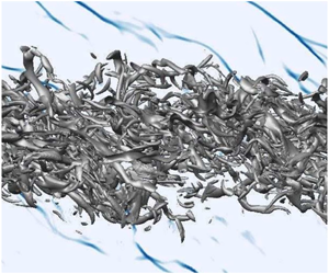
  $\unicode[STIX]{x0394}t=2$. The time duration is enough to cover the integral time scale in the self-similar stage. The statistics points for each instantaneous flow field are sampled from the region where the turbulence is fully developed (Yu & Lu Reference Yu and Lu2019). We have examined that increasing the data samples does not change the statistical results. Moreover, figure 2 shows the coherent structures obtained by isosurfaces of the second invariant of the VGT. The presence of shocklets is also shown in figure 2 based on the velocity dilatation (Hadjadj & Kudryavtsev Reference Hadjadj and Kudryavtsev2005). It is found that the shocklets exist outside the mixing layer, which is consistent with previous observation (Vaghefi et al. Reference Vaghefi, Nik, Pisciuneri and Madnia2013).
3 Lagrangian equations of the filtered velocity gradient tensor invariants
3.1 Invariants and local flow topologies
The eigenvalues  $\unicode[STIX]{x1D6EC}_{i}$ of the VGT
  $\unicode[STIX]{x1D63C}$ with components
  $\unicode[STIX]{x1D608}_{ij}=\unicode[STIX]{x2202}u_{i}/\unicode[STIX]{x2202}x_{j}$ are obtained as solutions of the characteristic equation
 $$\begin{eqnarray}\unicode[STIX]{x1D6EC}_{i}^{3}+P\unicode[STIX]{x1D6EC}_{i}^{2}+Q\unicode[STIX]{x1D6EC}_{i}+R=0,\end{eqnarray}$$
 where  $P$,
$P$,  $Q$ and
  $R$ are the first, second and third invariants of
  $\unicode[STIX]{x1D63C}$, described as
 $$\begin{eqnarray}\displaystyle & \displaystyle P=-\unicode[STIX]{x1D61A}_{ii}=-\unicode[STIX]{x1D703}, & \displaystyle\end{eqnarray}$$
 $$\begin{eqnarray}\displaystyle & \displaystyle Q={\textstyle \frac{1}{2}}(P^{2}-\unicode[STIX]{x1D61A}_{ij}\unicode[STIX]{x1D61A}_{ji}-\unicode[STIX]{x1D61E}_{ij}\unicode[STIX]{x1D61E}_{ji}), & \displaystyle\end{eqnarray}$$
 $$\begin{eqnarray}\displaystyle & \displaystyle R={\textstyle \frac{1}{3}}(-P^{3}+3PQ-\unicode[STIX]{x1D61A}_{ij}\unicode[STIX]{x1D61A}_{jk}\unicode[STIX]{x1D61A}_{ki}-3\unicode[STIX]{x1D61E}_{ij}\unicode[STIX]{x1D61E}_{jk}\unicode[STIX]{x1D61A}_{ki}), & \displaystyle\end{eqnarray}$$
 where  $\unicode[STIX]{x1D703}$ is the dilatation,
  $\unicode[STIX]{x1D61A}_{ij}=(\unicode[STIX]{x1D608}_{ij}+\unicode[STIX]{x1D608}_{ji})/2$ is the symmetric strain-rate tensor
  $\unicode[STIX]{x1D64E}$ and
  $\unicode[STIX]{x1D61E}_{ij}=(\unicode[STIX]{x1D608}_{ij}-\unicode[STIX]{x1D608}_{ji})/2$ is the skew-symmetric rotation-rate tensor
  $\unicode[STIX]{x1D652}$. The invariants of
  $\unicode[STIX]{x1D64E}$ are given by
 $$\begin{eqnarray}P_{S}=P=-\unicode[STIX]{x1D61A}_{ii},\quad Q_{S}={\textstyle \frac{1}{2}}(P_{S}^{2}-\unicode[STIX]{x1D61A}_{ij}\unicode[STIX]{x1D61A}_{ji}),\quad R_{S}={\textstyle \frac{1}{3}}(-P_{S}^{3}+3P_{S}Q_{S}-\unicode[STIX]{x1D61A}_{ij}\unicode[STIX]{x1D61A}_{jk}\unicode[STIX]{x1D61A}_{ki}).\end{eqnarray}$$
 The first and third invariants of  $\unicode[STIX]{x1D652}$ are zero and its second invariant is
 $$\begin{eqnarray}Q_{W}=-{\textstyle \frac{1}{2}}\unicode[STIX]{x1D61E}_{ij}\unicode[STIX]{x1D61E}_{ji}={\textstyle \frac{1}{4}}\unicode[STIX]{x1D714}_{i}\unicode[STIX]{x1D714}_{i},\end{eqnarray}$$
 where  $\unicode[STIX]{x1D714}_{i}$ is the vorticity and
  $Q_{W}$ is positive definite. Thus, we can obtain
 $$\begin{eqnarray}Q=Q_{S}+Q_{W},\quad R=R_{S}-E_{P},\end{eqnarray}$$
 where  $E_{P}=\frac{1}{4}\unicode[STIX]{x1D714}_{i}\unicode[STIX]{x1D61A}_{ij}\unicode[STIX]{x1D714}_{j}$ is enstrophy production rate. Therefore,
  $Q$ represents the competition between dissipation and enstrophy. The fluid particles locate in the enstrophy-dominant regions when
  $Q>0$ and in the dissipation-dominant regions when
  $Q<0$. And
  $R$ represents the competition between dissipation production and enstrophy production. The fluid particles locate in the dissipation-production-dominant regions when
  $R>0$ and in the enstrophy-production-dominant regions when
  $R<0$. The invariants
  $Q$ and
  $R$ describe the characteristics of dissipation and enstrophy of the local fluid.
The flow topology of turbulent flow can be investigated in the  $P$–
$P$– $Q$–
$Q$– $R$ space using critical point theory (Chong et al. Reference Chong, Perry and Cantwell1990). The discriminant of (3.1) is given by
 $$\begin{eqnarray}\unicode[STIX]{x1D6E5}=27R^{2}+(4P^{3}-18PQ)R+(4Q^{3}-P^{2}Q^{2}).\end{eqnarray}$$
 The surface  $\unicode[STIX]{x1D6E5}=0$ divides the
  $P$–
$P$– $Q$–
$Q$– $R$ space into two regions. In the focal region (
 $\unicode[STIX]{x1D6E5}>0$),
  $\unicode[STIX]{x1D608}_{ij}$ has one real and two complex-conjugate eigenvalues and the fluid particle sits on a part of structure that has a rotational character. In the non-focal region (
 $\unicode[STIX]{x1D6E5}\leqslant 0$),
  $\unicode[STIX]{x1D608}_{ij}$ has three real eigenvalues and the supporting structure is purely straining. Further, in the region with
  $\unicode[STIX]{x1D6E5}>0$,
  $\unicode[STIX]{x1D608}_{ij}$ has purely imaginary eigenvalues on the surface
  $PQ-R=0$ and the flow pattern is two-dimensional on the surface
  $R=0$ (Chong et al. Reference Chong, Perry and Cantwell1990). Thus, the surfaces
  $\unicode[STIX]{x1D6E5}=0$,
  $PQ-R=0$ and
  $R=0$ divide the
  $P$–
$P$– $Q$–
$Q$– $R$ space into different regions, and each of these regions corresponds to a topology.
Owing to the spatial complexity of different topologies in the  $P$–
$P$– $Q$–
$Q$– $R$ space, it is convenient to analyse the flow topology in the
  $Q$–
$Q$– $R$ plane for a specific value of
  $P$ (Suman & Girimaji Reference Suman and Girimaji2010; Wang & Lu Reference Wang and Lu2012; Vaghefi & Madnia Reference Vaghefi and Madnia2015). For
  $P=0$, the curves divide the
  $Q$–
$Q$– $R$ plane into four regions corresponding to two focal (UFC and SFS) and two non-focal (UN/S/S and SN/S/S) topologies. For
  $P>0$, three focal topologies (UFC, SFS and SFC) and three non-focal topologies (UN/S/S, SN/S/S and SN/SN/SN) are identified. And for
  $P<0$, six possible topologies are distinguished, three of them being focal (UFC, SFS and UFS) and three of them non-focal (UN/S/S, SN/S/S and UN/UN/UN). The descriptions of the topologies are shown in figure 3 and the corresponding acronyms are given in table 2.

Figure 3. Topological classification in the  $Q$–
$Q$– $R$ plane for: (a)
  $P=0$, incompressible region; (b)
  $P>0$, compressed region; and (c)
  $P<0$, expanded region. The acronyms are described in table 2.
Table 2. Description of acronyms of various local topologies in the  $P$–
$P$– $Q$–
$Q$– $R$ space.

3.2 Evolution equations of the invariants of the filtered velocity gradient
The time evolution of the filtered velocity gradient  $\widetilde{\unicode[STIX]{x1D608}}_{ij}=\unicode[STIX]{x2202}\widetilde{u}_{i}/\unicode[STIX]{x2202}x_{j}$, where
  $\widetilde{u}_{i}$ is the Favre filtered velocity defined as
  $\widetilde{u}_{i}=\overline{\unicode[STIX]{x1D70C}u_{i}}/\overline{\unicode[STIX]{x1D70C}}$ with the overbar representing the filtered quantity, can be obtained by taking the gradient of the Favre filtered Navier–Stokes equations, which are commonly used in large-eddy simulation. The resulting equation reads
 $$\begin{eqnarray}\frac{\text{D}\unicode[STIX]{x1D608}_{ij}}{\text{D}t}+\unicode[STIX]{x1D608}_{ik}\unicode[STIX]{x1D608}_{kj}=-\unicode[STIX]{x1D60F}_{ij}+\unicode[STIX]{x1D61D}_{ij}+\unicode[STIX]{x1D60E}_{ij},\end{eqnarray}$$
 where  $\text{D}/\text{D}t$ denotes the material derivative. The tilde on the gradient is ignored for convenience, but it is understood that it can be either unfiltered or filtered depending on the context. Here
  $\unicode[STIX]{x1D60F}_{ij}$,
  $\unicode[STIX]{x1D61D}_{ij}$ and
  $\unicode[STIX]{x1D60E}_{ij}$ in (3.9) stand for the components of the pressure effect term
  $\unicode[STIX]{x1D643}$, the viscous term
  $\unicode[STIX]{x1D651}$ and the subgrid effect term
  $\unicode[STIX]{x1D642}$, respectively, and are defined by
 $$\begin{eqnarray}\unicode[STIX]{x1D60F}_{ij}=\frac{\unicode[STIX]{x2202}}{\unicode[STIX]{x2202}x_{j}}\left(\frac{1}{\unicode[STIX]{x1D70C}}\frac{\unicode[STIX]{x2202}p}{\unicode[STIX]{x2202}x_{i}}\right),\quad \unicode[STIX]{x1D61D}_{ij}=\frac{\unicode[STIX]{x2202}}{\unicode[STIX]{x2202}x_{j}}\left(\frac{1}{\unicode[STIX]{x1D70C}}\frac{\unicode[STIX]{x2202}\unicode[STIX]{x1D70E}_{ik}}{\unicode[STIX]{x2202}x_{k}}\right),\quad \unicode[STIX]{x1D60E}_{ij}=\frac{\unicode[STIX]{x2202}}{\unicode[STIX]{x2202}x_{j}}\left(\frac{1}{\unicode[STIX]{x1D70C}}\frac{\unicode[STIX]{x2202}\unicode[STIX]{x1D70F}_{ik}}{\unicode[STIX]{x2202}x_{k}}\right),\end{eqnarray}$$
 where  $\unicode[STIX]{x1D70E}_{ij}$ is the viscous stress tensor and
  $\unicode[STIX]{x1D70F}_{ij}$ is the SGS stress tensor defined as
 $$\begin{eqnarray}\unicode[STIX]{x1D70F}_{ij}=\overline{\unicode[STIX]{x1D70C}}(\widetilde{u_{i}u_{j}}-\widetilde{u}_{i}\widetilde{u}_{j}).\end{eqnarray}$$
 Based on the definitions of  $P$,
$P$,  $Q$ and
  $R$, the evolution equations for
  $P$,
$P$,  $Q$ and
  $R$ are derived as
 $$\begin{eqnarray}\frac{\text{D}P}{\text{D}t}=(P^{2}-2Q)+\text{tr}(\unicode[STIX]{x1D643})-\text{tr}(\unicode[STIX]{x1D651})-\text{tr}(\unicode[STIX]{x1D642})=PS+PH+PV+PG,\end{eqnarray}$$
 $$\begin{eqnarray}\displaystyle \frac{\text{D}Q}{\text{D}t} & = & \displaystyle (PQ-3R)+(P\,\text{tr}(\unicode[STIX]{x1D643})+\text{tr}(\unicode[STIX]{x1D63C}\unicode[STIX]{x1D643}))-(P\,\text{tr}(\unicode[STIX]{x1D651})+\text{tr}(\unicode[STIX]{x1D63C}\unicode[STIX]{x1D651}))\nonumber\\ \displaystyle & & \displaystyle -\,(P\,\text{tr}(\unicode[STIX]{x1D642})+\text{tr}(\unicode[STIX]{x1D63C}\unicode[STIX]{x1D642}))\nonumber\\ \displaystyle & = & \displaystyle QS+QH+QV+QG\end{eqnarray}$$
and
 $$\begin{eqnarray}\displaystyle \frac{\text{D}R}{\text{D}t} & = & \displaystyle PR+(Q\,\text{tr}(\unicode[STIX]{x1D643})+P\,\text{tr}(\unicode[STIX]{x1D63C}\unicode[STIX]{x1D643})+\text{tr}(\unicode[STIX]{x1D63C}^{2}\unicode[STIX]{x1D643}))-(Q\,\text{tr}(\unicode[STIX]{x1D651})+P\,\text{tr}(\unicode[STIX]{x1D63C}\unicode[STIX]{x1D651})+\text{tr}(\unicode[STIX]{x1D63C}^{2}\unicode[STIX]{x1D651}))\nonumber\\ \displaystyle & & \displaystyle -\,(Q\,\text{tr}(\unicode[STIX]{x1D642})+P\,\text{tr}(\unicode[STIX]{x1D63C}\unicode[STIX]{x1D642})+\text{tr}(\unicode[STIX]{x1D63C}^{2}\unicode[STIX]{x1D642}))\nonumber\\ \displaystyle & = & \displaystyle RS+RH+RV+RG.\end{eqnarray}$$
 The meanings of the source terms in (3.12)–(3.14) are described as follows:  $PS$,
$PS$,  $QS$ and
  $RS$ are the interaction terms among the invariants;
  $PH$,
$PH$,  $QH$ and
  $RH$ are the contributions due to the pressure effects;
  $PV$,
$PV$,  $QV$ and
  $RV$ are the viscous effect terms; and
  $PG$,
$PG$,  $QG$ and
  $RG$ are the subgrid effect terms. Thus, the evolution of the filtered VGT of a fluid element is dictated by the combination of four effects. The subgrid effect terms are expected to be significantly smaller than the other terms when the filter scale is comparable to the viscous scale, and the viscous effects are expected to be quite small when the scale belongs to the inertial scale.
4 The Schur decomposition of the velocity gradient tensor
The evolutions of the invariants are unclosed due to the viscous effects and the highly non-local pressure field. To investigate the local and the non-local effects, respectively, an additive decomposition of the VGT is employed to get better insights into turbulence processes (Keylock Reference Keylock2018). The VGT is decomposed into its normal part  $\unicode[STIX]{x1D63D}$ (characterized by the eigenvalues) and non-normal part
  $\unicode[STIX]{x1D63E}$ (characterizing the tensor asymmetries) as
 $$\begin{eqnarray}\unicode[STIX]{x1D63C}=\unicode[STIX]{x1D63D}+\unicode[STIX]{x1D63E}.\end{eqnarray}$$
To obtain the decomposition, the complex Schur transform of the VGT is introduced,
 $$\begin{eqnarray}\unicode[STIX]{x1D63C}=\unicode[STIX]{x1D650}\unicode[STIX]{x1D64F}\unicode[STIX]{x1D650}^{\ast },\end{eqnarray}$$
 where the superscript  $^{\ast }$ is the conjugate transpose. The tensor
  $\unicode[STIX]{x1D650}$ is unitary, with
  $\unicode[STIX]{x1D650}\unicode[STIX]{x1D650}^{\ast }=\unicode[STIX]{x1D644}$, where
  $\unicode[STIX]{x1D644}$ is the identity matrix. The tensor
  $\unicode[STIX]{x1D64F}$ is an upper triangular tensor with
  $\unicode[STIX]{x1D64F}=\unicode[STIX]{x1D71E}+\unicode[STIX]{x1D649}$, where
  $\unicode[STIX]{x1D649}$ is a strictly upper triangular tensor and
  $\unicode[STIX]{x1D71E}$ is a diagonal matrix and the diagonal elements of
  $\unicode[STIX]{x1D71E}$ are the eigenvalues of
  $\unicode[STIX]{x1D63C}$. The normal and non-normal tensors can be written as
 $$\begin{eqnarray}\unicode[STIX]{x1D63D}=\unicode[STIX]{x1D650}\unicode[STIX]{x1D71E}\unicode[STIX]{x1D650}^{\ast },\quad \unicode[STIX]{x1D63E}=\unicode[STIX]{x1D650}\unicode[STIX]{x1D649}\unicode[STIX]{x1D650}^{\ast }.\end{eqnarray}$$
 The normal part  $\unicode[STIX]{x1D63D}$ is related to the dynamics driven by the eigenvalues of the VGT and acts locally, and the non-normal part
  $\unicode[STIX]{x1D63E}$ is related to the vortical structures and the non-local effects of fluid dynamics. In reality, the advantage of the Schur decomposition is that it contains the information of the eigenvalues of the VGT, while the conventional decomposition of the VGT into its symmetric and skew-symmetric parts does not include any information about the invariants of the VGT. The relevant information is helpful in the construction of reliable SGS models (Chacin & Cantwell Reference Chacin and Cantwell2000; Meneveau Reference Meneveau2011).
The strain-rate tensor and the rotation-rate tensor of  $\unicode[STIX]{x1D63D}$ and
  $\unicode[STIX]{x1D63E}$ can be given as
 $$\begin{eqnarray}\unicode[STIX]{x1D63D}=\unicode[STIX]{x1D64E}^{B}+\unicode[STIX]{x1D652}^{B}\quad \text{and}\quad \unicode[STIX]{x1D63E}=\unicode[STIX]{x1D64E}^{C}+\unicode[STIX]{x1D652}^{C},\end{eqnarray}$$
and in this case we have
 $$\begin{eqnarray}\Vert \unicode[STIX]{x1D64E}\Vert ^{2}=\Vert \unicode[STIX]{x1D64E}^{B}\Vert ^{2}+\Vert \unicode[STIX]{x1D64E}^{C}\Vert ^{2},\quad \Vert \unicode[STIX]{x1D652}\Vert ^{2}=\Vert \unicode[STIX]{x1D652}^{B}\Vert ^{2}+\Vert \unicode[STIX]{x1D652}^{C}\Vert ^{2},\end{eqnarray}$$
 where  $\Vert \unicode[STIX]{x1D64E}\Vert =\sqrt{\text{tr}(\unicode[STIX]{x1D64E}\unicode[STIX]{x1D64E}^{\ast })}$ is the Frobenius norm. The invariants of
  $\unicode[STIX]{x1D63D}$ and
  $\unicode[STIX]{x1D63E}$, i.e.
  $P^{B}$,
  $Q^{B}$ and
  $R^{B}$, and
  $P^{C}$,
  $Q^{C}$ and
  $R^{C}$, respectively, are given by
 $$\begin{eqnarray}\left.\begin{array}{@{}c@{}}P^{B}=P_{S}^{B}=P,\quad P^{C}=P_{W}^{B}=P_{S}^{C}=P_{W}^{C}=0,\\[6.0pt] Q^{B}=Q_{S}^{B}+Q_{W}^{B}=Q_{S}+Q_{W}=Q,\quad Q^{C}=Q_{S}^{C}+Q_{W}^{C}=0,\\[6.0pt] R^{B}=R_{S}^{B}-E_{P}^{B}=R_{S}-E_{P}=R,\quad R^{C}=R_{S}^{C}-E_{P}^{C}=0,\end{array}\right\}\end{eqnarray}$$
 where  $P_{S}^{B}$ is the first invariant of
  $\unicode[STIX]{x1D64E}^{B}$ and the other invariants are defined similarly. It is noted that the invariants of tensors
  $\unicode[STIX]{x1D63C}$ and
  $\unicode[STIX]{x1D63D}$ are identical, whereas the invariants of tensors
  $\unicode[STIX]{x1D64E}^{A}$ and
  $\unicode[STIX]{x1D64E}^{B}$ are different except where the tensor
  $\unicode[STIX]{x1D63C}$ is normal and
  $\unicode[STIX]{x1D63C}=\unicode[STIX]{x1D63D}$.
From the above identities,  $Q^{B}=Q$ and
  $R^{B}=R$. The dynamics of the VGT invariants only describes the behaviour of the normal part of the VGT. The component terms of the second and third invariants when
  $\Vert \unicode[STIX]{x1D63E}\Vert \neq 0$ will introduce non-normal effects into consideration.
The Schur decomposition is related directly to the discriminant of the VGT. The discriminant defines a sharp threshold between real eigenvalue regions and those with a conjugate pair. There are no imaginary parts in  $\unicode[STIX]{x1D63D}$ when
  $\unicode[STIX]{x1D6E5}\leqslant 0$ and in this case we have
 $$\begin{eqnarray}R^{B}=R_{S}^{B}=R,\quad Q^{B}=Q_{S}^{B}=Q.\end{eqnarray}$$
 However,  $\unicode[STIX]{x1D608}_{ij}$ has one real and two complex-conjugate eigenvalues when
  $\unicode[STIX]{x1D6E5}>0$ and the normal part
  $\unicode[STIX]{x1D63D}$ and the non-normal part
  $\unicode[STIX]{x1D63E}$ are complex matrices. All enstrophy comes from the non-normal term when
  $\unicode[STIX]{x1D6E5}\leqslant 0$, while the enstrophy arises from both the normal and the non-normal terms when
  $\unicode[STIX]{x1D6E5}>0$.
5 Results and discussion
5.1 Local flow topology in the inertial range
The local flow topology of the filtered VGT in compressible turbulence is investigated first. The average energy spectrum in the streamwise direction at the centreline obtained from the DNS data is shown in figure 4. Here, the average energy spectrum at the centreline is defined as
 $$\begin{eqnarray}\hat{E}(k_{x})=\left[\frac{1}{L_{z}}\int _{0}^{L_{z}}\hat{E}(k_{x},z)\hat{E}^{\ast }(k_{x},z)\,\text{d}z\right]^{1/2},\end{eqnarray}$$
 where  $\hat{E}(k_{x},z)$ is the Fourier transform of the turbulent kinetic energy in the streamwise direction at the centreline,
  $k_{x}$ is the wavenumber in the streamwise direction,
  $\hat{E}^{\ast }$ is the conjugate transpose of
  $\hat{E}$ and
  $L_{z}$ is the computational domain length in the spanwise direction. Based on the spectrum, the cutoff wavenumbers of
  $0.07<k\unicode[STIX]{x1D702}<0.33$ are associated with inertial range behaviour and the corresponding filter widths are
  $19\unicode[STIX]{x1D702}<d<90\unicode[STIX]{x1D702}$. A three-dimensional, spatial low-pass box filter is employed to analyse the local flow topology of the filtered VGT. Moreover, a filter width of
  $30\unicode[STIX]{x1D702}$ is used in the following analysis to study the subgrid effects on the filtered VGT.

Figure 4. Average energy spectrum in the streamwise direction at the centreline at  $t=1200$. The dashed line indicates a
  $-5/3$ slope showing an inertial range.

Figure 5. The j.p.d.f.s of  $Q$ and
  $R$ for (a)
  $P=0$, (b)
  $P/Q_{0}^{1/2}=0.3$ and (c)
  $P/Q_{0}^{1/2}=-0.3$. The probability isocontours contains 90 % of the data. The black dashed lines are
  $\unicode[STIX]{x1D6E5}=0$; the solid lines represent the unfiltered velocity fields; and the dash-dotted lines represent the filtered velocity fields with a filter width of
  $30\unicode[STIX]{x1D702}$.
The local state of filtered turbulence in compressible flows can be characterized by the j.p.d.f.s of  $Q$ and
  $R$ for a selected
  $P$, i.e.
  ${\mathcal{P}}(R,Q)$. In the following analysis, the VGT invariants are normalized by the quantities related to
  $Q_{0}=\langle Q_{W0}\rangle$, where
  $Q_{W0}$ is the value of
  $Q_{W}$ obtained from unfiltered or filtered flow fields at the centreline. Hence, the invariants
  $P$,
$P$,  $Q$ and
  $R$ and the time
  $t$ are normalized by
  $Q_{0}^{1/2}$,
  $Q_{0}$,
  $Q_{0}^{3/2}$ and
  $Q_{0}^{-1/2}$, respectively. Three typical values of
  $P$, i.e.
  $P/Q_{0}^{1/2}=0$, 0.3 and
  $-0.3$, are chosen to compare the statistics in incompressible, compressed and expanded regions. Statistics are calculated for all the points with
  $P/Q_{0}^{1/2}\pm \unicode[STIX]{x1D716}$ around the above levels. The threshold of
  $\unicode[STIX]{x1D716}=0.01$ is chosen in our study, and it is examined that using smaller thresholds does not change the statistics of the flow.
The j.p.d.f.s of  $Q$ and
  $R$ computed from the unfiltered and filtered VGT with a filter width of
  $30\unicode[STIX]{x1D702}$ in the inertial range are shown in figure 5. For the unfiltered case, the iso-contour lines maintain a universal teardrop shape around the origin and focal structures (63.9 %) are more than non-focal structures (36.1 %), consistent with previous studies for different flow configurations (Soria et al. Reference Soria, Sondergaard, Cantwell, Chong and Perry1994; Blackburn et al. Reference Blackburn, Mansour and Cantwell1996; Chong et al. Reference Chong, Soria, Perry, Chacin, Cantwell and Na1998; Ooi et al. Reference Ooi, Martin, Soria and Chong1999; da Silva & Pereira Reference da Silva and Pereira2008; Suman & Girimaji Reference Suman and Girimaji2010; Wang & Lu Reference Wang and Lu2012; Lozano-Durán et al. Reference Lozano-Durán, Holzner and Jiménez2016). It is noted that extended tails, which are called Vieillefosse tails, appear along the curves
  $\unicode[STIX]{x1D6E5}=0$ in the fourth quadrant, reflecting a dominance of dissipation production over enstrophy production in the dissipation-dominated regions. The j.p.d.f.s are more symmetrical with respect to
  $R=0$ in the locally compressed regions and exhibit more skewed shapes with respect to those for
  $P=0$ in the locally expanded regions. Compared with the unfiltered velocity fields, the iso-contour lines tend to broaden slightly in the inertial range, which means that
  $R$ is stronger than the unfiltered case for a given
  $Q$. The results also indicate that the normalization with
  $Q_{0}$ is appropriate. Without the normalization, the values of the invariants for the filtered cases are strongly reduced by several orders of magnitude with respect to the unfiltered case, since the strong gradients and intermittent events are mostly caused by the small-scale structures of turbulence.
In order to quantify the statistical properties of the j.p.d.f.s as shown in figure 5, the probability of occurrence of different topologies in table 2 for different levels of  $P$ is examined. The occurrence of each topology is calculated by volume ratio, which is the percentage of volume of each topology in the total volume. For each level of
  $P_{0}$, all the points with
  $P=P_{0}\pm \unicode[STIX]{x1D716}$ are chosen as data samples. The variations of the volume ratios for four topologies at
  $P=0$ versus
  $\unicode[STIX]{x1D716}$ are shown in figure 6. The volume ratios for SFC, SN/SN/SN, UFS and UN/UN/UN topologies at
  $P=0$ are zero in theory, but obvious errors occur for SFC and UFS topologies when the threshold
  $\unicode[STIX]{x1D716}$ is large. Based on our careful tests, it is identified from figure 6 that the statistical errors are quite small (less than 0.1 %) for
  $\unicode[STIX]{x1D716}<0.02$. Therefore, a threshold of
  $\unicode[STIX]{x1D716}=0.01$ is used in the present study.

Figure 6. The variations of the volume ratios for SFC, SN/SN/SN, UFS and UN/UN/UN topologies at  $P=0$ versus threshold
  $\unicode[STIX]{x1D716}$ for (a) unfiltered case and (b) filtered case with a filter width of
  $30\unicode[STIX]{x1D702}$.
Figure 7 shows the volume ratio of each topology conditioned on the dilatation  $P$ for unfiltered and filtered cases with a threshold of
  $\unicode[STIX]{x1D716}=0.01$. It is seen from figure 7(a) and (b) that, in the incompressible regions with
  $P=0$, the most probable topology is SFS (37.6 %), after that UN/S/S and UFC (26.9 % and 26.6 %), and the least probable topology is SN/S/S (8.9 %), consistent with those reported by Suman & Girimaji (Reference Suman and Girimaji2010) and Vaghefi & Madnia (Reference Vaghefi and Madnia2015). Compared to the incompressible regions, more fluid particles tend to be located in stable topologies (SN/S/S, SFC and SN/SN/SN) and fewer fluid particles in unstable topologies (UN/S/S, UFS and UN/UN/UN), which means that the locally compressed region is favourable to stable topologies. On the contrary, the locally expanded region is favourable to unstable topologies. The volume ratios of UFC topology and UN/S/S topology conditioned on the dilatation in the inertial range are shown in figure 7(c). Compared with the unfiltered case, a decrease of UN/S/S topology and an increase of UFC topology are observed for the entire flow domain. The changes of the other topologies in the inertial range with the dilatation are similar to the unfiltered results, which are not shown here.

Figure 7. (a) The volume ratios occupied by UFC, UN/S/S, SN/S/S and SFS topologies conditioned on  $P$ for the unfiltered case. (b) The volume ratios occupied by SFC, SN/SN/SN, UFS and UN/UN/UN topologies conditioned on
  $P$ for the unfiltered case. (c) The volume ratios occupied by UFC and UN/S/S topologies for the unfiltered case and the filtered case with a filter width of
  $30\unicode[STIX]{x1D702}$.
5.2 The dynamics of the filtered velocity gradient tensor
The compressibility effect on the mean topological evolution in the inertial range is investigated. In order to quantify the effects of the pressure, the viscous, the subgrid and the interaction terms among the invariants on the evolution of the filtered velocity gradient invariants  $Q$ and
  $R$ for a selected
  $P$ in a statistically robust and meaningful way, a vector associated with the evolution of the filtered VGT in the
  $Q$–
$Q$– $R$ plane is introduced and defined as
 $$\begin{eqnarray}\boldsymbol{V}=\left\langle \frac{\text{D}R}{\text{D}t},\frac{\text{D}Q}{\text{D}t}\right\rangle _{R,Q}=\boldsymbol{V}_{S}+\boldsymbol{V}_{H}+\boldsymbol{V}_{V}+\boldsymbol{V}_{G},\end{eqnarray}$$
with
 $$\begin{eqnarray}\boldsymbol{V}_{S}=\langle RS,QS\rangle _{R,Q},\end{eqnarray}$$
 where  $\langle \cdot \rangle _{R,Q}$ denotes the conditional mean at point
  $(R,Q)$. Here
  $\boldsymbol{V}_{H}$,
  $\boldsymbol{V}_{V}$ and
  $\boldsymbol{V}_{G}$ are defined similarly. The dynamics of the filtered VGT are composed of four different subterms representing the pressure effect, the viscous effect, the subgrid effect and the interaction among the invariants, respectively. Such a decomposition can help us in pinpointing the role of each of these effects as a function of the dilatation.
5.2.1 The vector plots
The dynamics of the filtered VGT for a selected  $P$ can be visualized by plotting the fields of the vector
  $\boldsymbol{V}$ in the
  $Q$–
$Q$– $R$ plane and using the length of the vector to show the magnitude, which has been used in previous studies (van der Bos et al. Reference van der Bos, Tao, Meneveau and Katz2002; Chu & Lu Reference Chu and Lu2013). The conditional mean trajectories of the vector
  $\boldsymbol{V}$ are shown in figure 8 for different dilatations. The trajectories show significant deviations for different dilatations. The dynamics of the local flow topology in the incompressible regions describe clockwise cycles around the origin in almost closed trajectories, which is consistent with previous studies (Chong et al. Reference Chong, Soria, Perry, Chacin, Cantwell and Na1998; Martin et al. Reference Martin, Ooi, Chong and Soria1998; Lozano-Durán et al. Reference Lozano-Durán, Holzner and Jiménez2015, Reference Lozano-Durán, Holzner and Jiménez2016), while the conditional mean trajectories of
  $\boldsymbol{V}$ spiral outwards in the locally compressed regions and inwards in the locally expanded regions. As the level of compression is increased, the outward spiral of
  $\boldsymbol{V}$ becomes more obvious. By comparing figure 8(a) with figure 8(b), the results based on
  $P/Q_{0}^{1/2}=0.3$ and
  $P/Q_{0}^{1/2}=1.0$ are qualitatively consistent with each other, which indicates that the threshold value
  $P/Q_{0}^{1/2}=0.3$ is enough to reflect the characteristics of the dynamics of the filtered VGT in the locally compressed regions. The magnitudes of
  $\boldsymbol{V}$ increase with increasing distance from the origin. The directions of
  $\boldsymbol{V}$ along the Vieillefosse tails are strongly associated with the dilatations. The vectors
  $\boldsymbol{V}$ point towards the origin in the locally expanded regions and point away from the origin in the locally compressed regions along the Vieillefosse tail, while the vector magnitude remains relatively small along the Vieillefosse tail in the incompressible regions.

Figure 8. Conditional mean trajectories of  $\boldsymbol{V}$ by use of the vectors for demonstration for (a)
  $P=0$, (b)
  $P/Q_{0}^{1/2}=0.3$, (c)
  $P/Q_{0}^{1/2}=1.0$ and (d)
  $P/Q_{0}^{1/2}=-0.3$. The scales for the vector magnitude are indicated in the upper right corner in each panel. The red lines indicate the streamlines in the
  $Q$–
$Q$– $R$ plane. Only values where
  ${\mathcal{P}}(R,Q)>10^{-4}$ are plotted.

Figure 9. Conditional mean trajectories of the interaction term among the invariants  $\boldsymbol{V}_{S}$ by use of the vectors for demonstration for (a)
  $P=0$, (b)
  $P/Q_{0}^{1/2}=0.3$ and (c)
  $P/Q_{0}^{1/2}=-0.3$. The scales for the vector magnitude are indicated in the upper right corner in each panel. Only values where
  ${\mathcal{P}}(R,Q)>10^{-4}$ are plotted.
The components of the evolution of invariants are analysed to understand the results presented above. The conditional mean trajectories of the vector  $\boldsymbol{V}_{S}$ in the
  $Q$–
$Q$– $R$ plane are shown in figure 9. It is seen that
  $Q$ tends to increase in the enstrophy-production-dominated regions (i.e.
  $R<0$) and to decrease in the dissipation-production-dominated regions (i.e.
  $R>0$). Such properties are attributed to the vortex stretching and the self-amplification of the strain-rate tensor (Cantwell Reference Cantwell1992; Chu & Lu Reference Chu and Lu2013). It is seen from (3.13) and (3.14) that, compared with the incompressible regions,
  $PQ$ and
  $PR$ are involved in the interaction term among the invariants, which tends to amplify the magnitude of the rate of change of the invariants in the locally compressed regions and to reduce the magnitude in the locally expanded regions.
The conditional mean trajectories of the vector  $\boldsymbol{V}_{H}$ in the
  $Q$–
$Q$– $R$ plane are shown in figure 10. On average, the enstrophy production rate tends to increase in the enstrophy-production-dominated regions and the dissipation production rate tends to increase in the dissipation-production-dominated regions due to the pressure effect, which reveals that the pressure effect term leads to the amplification of
  $|R|$. Compared with the incompressible regions,
  $Q$ tends to decrease in the locally compressed regions and to increase in the locally expanded regions on average. Moreover, the pressure effect leads to the local topology of fluid particles changing from the focal regions to the non-focal regions in the locally compressed regions, i.e. from SFC to UFC to UN/S/S or from SFS to SN/S/S, while the pressure effect leads to the local topology of fluid particles changing from the non-focal regions to the focal regions in the locally expanded regions, i.e. from SN/S/S to SFS to UFS or from UN/S/S to UFC.

Figure 10. Conditional mean trajectories of the pressure effect term  $\boldsymbol{V}_{H}$ by use of the vectors for demonstration for (a)
  $P=0$, (b)
  $P/Q_{0}^{1/2}=0.3$ and (c)
  $P/Q_{0}^{1/2}=-0.3$. The scales for the vector magnitude are indicated in the upper right corner in each panel. Only values where
  ${\mathcal{P}}(R,Q)>10^{-4}$ are plotted.
Figure 11 shows the conditional mean trajectories of the vector  $\boldsymbol{V}_{V}$. It is found that the viscous effect tends to attract the trajectories to the origin, consistent with previous findings in isotropic turbulence (van der Bos et al. Reference van der Bos, Tao, Meneveau and Katz2002; Chevillard et al. Reference Chevillard, Meneveau, Biferale and Toschi2008; Danish & Meneveau Reference Danish and Meneveau2018) and wall-bounded flows (Chu & Lu Reference Chu and Lu2013). There is no significant dependence of the results on compressibility in the inertial range. It is noted that the magnitude of
  $\boldsymbol{V}_{V}$ is smaller than other terms in the inertial range, and the viscous effect appears to be negligible at large scales.

Figure 11. Conditional mean trajectories of the viscous effect term  $\boldsymbol{V}_{V}$ by use of the vectors for demonstration for (a)
  $P=0$, (b)
  $P/Q_{0}^{1/2}=0.3$ and (c)
  $P/Q_{0}^{1/2}=-0.3$. The scales for the vector magnitude are indicated in the upper right corner in each panel. Only values where
  ${\mathcal{P}}(R,Q)>10^{-4}$ are plotted.
The conditional mean trajectories of the subgrid effect vectors  $\boldsymbol{V}_{G}$ in the
  $Q$–
$Q$– $R$ plane are shown in figure 12. As expected, the magnitude of
  $\boldsymbol{V}_{G}$ is larger than
  $\boldsymbol{V}_{V}$ in the inertial range. Hence, the subgrid effect exerts a non-negligible influence on the filtered velocity gradient dynamics. Significant differences in the direction of the vectors are observed for different dilatations. In the incompressible regions, the subgrid effect term leads to an increase of
  $R$ and a decrease of
  $Q$ in the enstrophy-production-dominated regions, while
  $\boldsymbol{V}_{G}$ is directed to the origin in the fourth quadrant and
  $\boldsymbol{V}_{G}$ has a small magnitude and ill-defined direction in the first quadrant. In the locally compressed regions, the characteristic of
  $\boldsymbol{V}_{G}$ is similar to
  $\boldsymbol{V}_{V}$. That is,
  $\boldsymbol{V}_{G}$ is directed to the origin in the entire
  $Q$–
$Q$– $R$ plane and the magnitudes of
  $\boldsymbol{V}_{G}$ are decreasing with decreasing distance to the origin. In the locally expanded regions, the direction of
  $\boldsymbol{V}_{G}$ is more irregular and the small magnitude and ill-defined directions of
  $\boldsymbol{V}_{G}$ are also found in the second quadrant. Moreover, it is noted that the contributions of the subgrid effect appear to be strong along the Vieillefosse tails in the fourth quadrant, where the subgrid effect is similar to the viscous effect, and attract the trajectories to the origin, which indicates that the subgrid effect is mostly dissipative in the inertial range. For the particles along the Vieillefosse tails, the energy transfer mechanism from the inertial scale to the subgrid scale is analogous to the diffusion mechanism, while the ill-defined directions of
  $\boldsymbol{V}_{G}$ in the incompressible regions and the locally expanded regions are not dissipative, resulting in a difficult mechanism in modelling the SGS tensors.

Figure 12. Conditional mean trajectories of the subgrid effect term  $\boldsymbol{V}_{G}$ by use of the vectors for demonstration for (a)
  $P=0$, (b)
  $P/Q_{0}^{1/2}=0.3$ and (c)
  $P/Q_{0}^{1/2}=-0.3$. The scales for the vector magnitude are indicated in the upper right corner in each panel. Only values where
  ${\mathcal{P}}(R,Q)>10^{-4}$ are plotted.
5.2.2 The flux measurements
To elucidate which terms are responsible for the change of the dynamics of the filtered VGT in statistics with dilatations, the study of the net effects of each term as a function of  $P$ is required. The total probability flux calculated across a closed boundary placed in the
  $Q$–
$Q$– $R$ plane is presented to quantify the effects of each term (Danish & Meneveau Reference Danish and Meneveau2018). As shown in figure 13, a circle centred at the origin is chosen to calculate the probability flux. The total flux crossing the circle can be obtained by
 $$\begin{eqnarray}{\mathcal{J}}=\oint _{c}\,({\mathcal{P}}\boldsymbol{V}\boldsymbol{\cdot }\boldsymbol{n})\,\text{d}S,\end{eqnarray}$$
 where  $c$ is the closed circle,
  $\boldsymbol{n}$ is the normal vector outward from the surface and
  ${\mathcal{J}}$ represents the total flux of probability density. Using the divergence theorem, we have
 $$\begin{eqnarray}{\mathcal{J}}=\iint \unicode[STIX]{x1D735}\boldsymbol{\cdot }({\mathcal{P}}\boldsymbol{V})\,\text{d}R\,\text{d}Q={\mathcal{J}}_{S}+{\mathcal{J}}_{H}+{\mathcal{J}}_{V}+{\mathcal{J}}_{G},\end{eqnarray}$$
 where  ${\mathcal{J}}_{S}$,
  ${\mathcal{J}}_{H}$,
  ${\mathcal{J}}_{V}$ and
  ${\mathcal{J}}_{G}$ are fluxes due to the divergence of
  ${\mathcal{P}}\boldsymbol{V}_{S}$,
  ${\mathcal{P}}\boldsymbol{V}_{H}$,
  ${\mathcal{P}}\boldsymbol{V}_{V}$ and
  ${\mathcal{P}}\boldsymbol{V}_{G}$, respectively. If the flux is positive, the dynamics leads to a net outward trend in the
  $Q$–
$Q$– $R$ plane, which is denoted as a ‘source-like’ behaviour, while the dynamics leads to a net inward trend and corresponds to a ‘sink-like’ behaviour if the flux is negative. The statistically stationary condition implies that the total flux must be zero for a closed surface in the
  $P$–
$P$– $Q$–
$Q$– $R$ space. The total flux is not zero in the
  $Q$–
$Q$– $R$ plane for a given
  $P$, while the fluxes in (5.5) can still evaluate the relative importance of the pressure effect, the viscous effect, the subgrid effect and the interaction between the invariants.

Figure 13. Representative circles with radii equal to 0.75 and 1.25 centred at the origin of the  $Q$–
$Q$– $R$ plane.
The fluxes are calculated numerically within the circles in the  $Q$–
$Q$– $R$ plane for a given
  $P$. It is noted that the results depend strongly on the radius of the circle, since
  ${\mathcal{P}}$ decreases rapidly with increasing radius. In order to minimize the effect of the radius of the circle, the fluxes are normalized as follows:
 $$\begin{eqnarray}\left.\begin{array}{@{}c@{}}\displaystyle {\mathcal{J}}_{S}^{\ast }=\frac{{\mathcal{J}}_{S}}{\sqrt{{\mathcal{J}}_{S}^{2}+{\mathcal{J}}_{H}^{2}+{\mathcal{J}}_{V}^{2}+{\mathcal{J}}_{G}^{2}}},\quad {\mathcal{J}}_{H}^{\ast }=\frac{{\mathcal{J}}_{H}}{\sqrt{{\mathcal{J}}_{S}^{2}+{\mathcal{J}}_{H}^{2}+{\mathcal{J}}_{V}^{2}+{\mathcal{J}}_{G}^{2}}},\\ \displaystyle {\mathcal{J}}_{V}^{\ast }=\frac{{\mathcal{J}}_{V}}{\sqrt{{\mathcal{J}}_{S}^{2}+{\mathcal{J}}_{H}^{2}+{\mathcal{J}}_{V}^{2}+{\mathcal{J}}_{G}^{2}}},\quad {\mathcal{J}}_{G}^{\ast }=\frac{{\mathcal{J}}_{G}}{\sqrt{{\mathcal{J}}_{S}^{2}+{\mathcal{J}}_{H}^{2}+{\mathcal{J}}_{V}^{2}+{\mathcal{J}}_{G}^{2}}}.\end{array}\right\}\end{eqnarray}$$
 The values of the fluxes lie between  $-1$ and
  $+1$ as a result of this normalization.
The normalized fluxes as a function of dilatation are presented in figure 14. It is found that the results are quite independent of radius in the range of 0.75 to 1.25, and the change of the fluxes mainly occurs at  $-0.3<P/Q_{0}^{1/2}<0.3$. Therefore, the threshold values
  $P/Q_{0}^{1/2}=\pm 0.3$ are reasonable to distinguish the expanded and compressed regions for the dynamics of the velocity gradients. The flux for the interaction term among the invariants is shown with the solid lines in figure 14. The results indicate that the compressibility effect is directly related to
  ${\mathcal{J}}_{S}$, which changes from negative to positive values on increasing the value of
  $P$. Substituting
  $\boldsymbol{V}_{S}=\langle RS,QS\rangle _{R,Q}=\langle PR,PQ-3R\rangle _{R,Q}$ into (5.5) we can obtain
 $$\begin{eqnarray}{\mathcal{J}}_{S}=2P+\iint (\boldsymbol{V}_{S}\boldsymbol{\cdot }\unicode[STIX]{x1D735}){\mathcal{P}}\,\text{d}R\,\text{d}Q,\end{eqnarray}$$
 which indicates that the flux for the interaction term is measured by  $P$.
$P$.
The flux for the pressure effect term is shown with the dashed lines in figure 14. It is found that  ${\mathcal{J}}_{H}$ increases with the increase of
  $P$ and remains relatively unchanged in the locally compressed regions. The flux for the pressure term is positive and acts as a source, which is related to the fact that
  $\boldsymbol{V}_{H}$ points away from the origin, leading to an amplification of
  $|R|$. Moreover, it is identified that the flux for the viscous term is negative and acts as a sink. The flux for the viscous term is relatively small and independent of the dilatation, indicating that the viscous effect is weak in the inertial range and insensitive to the dilatation.

Figure 14. Normalized fluxes as a function of the dilatation  $P$, with radius (a)
  $r=0.75$ and (b)
  $r=1.25$. The solid, dashed, dash-dotted and dotted lines represent the flux for the interaction term among the invariants (
 ${\mathcal{J}}_{S}^{\ast }$), the pressure effect term (
 ${\mathcal{J}}_{H}^{\ast }$), the viscous effect term (
 ${\mathcal{J}}_{V}^{\ast }$) and the subgrid effect term (
 ${\mathcal{J}}_{G}^{\ast }$), respectively.
The flux for the subgrid effect term is shown in figure 14 with the dotted lines. It is seen that  ${\mathcal{J}}_{G}$ decreases rapidly with the increase of
  $P$ in the locally expanded regions and remains a constant value in the locally compressed regions. Compared with the other terms, the flux for the subgrid effect term changes most with the dilatation. The flux for the subgrid effect term is negative in the locally compressed regions, which is related to the fact that the characteristic of
  $\boldsymbol{V}_{G}$ is similar to
  $\boldsymbol{V}_{V}$, leading to a ‘sink-like’ behaviour; while the flux is positive and acts as a source in the locally expanded regions when
  $P/Q_{0}^{1/2}<-0.18$ due to the ill-defined directions of
  $\boldsymbol{V}_{G}$ in the upper part of the
  $Q$–
$Q$– $R$ plane and mostly outward-pointing. Above all, the change of the flux for the subgrid effect term with the dilatation is offset by the flux for the pressure effect term and the flux for the interaction term among the invariants to establish stationary statistics. The fluxes are directly related to the compressibility of the flow especially in the locally expanded regions.
5.3 Schur decomposition of the filtered velocity gradient tensor
5.3.1 The effect of compressibility on non-normality
The Schur decomposition of the filtered VGT,  $\unicode[STIX]{x1D63C}=\unicode[STIX]{x1D63D}+\unicode[STIX]{x1D63E}$, is used to develop better insights into compressible turbulence in this section. Firstly, the relative importance of the normal and the non-normal tensors is analysed. It is legitimate to approximate the behaviour of the VGT with eigenvalue-based formulations if
  $\unicode[STIX]{x1D63E}$ is small while the non-normality should be considered in the dynamics of the VGT if
  $\unicode[STIX]{x1D63E}$ is important. A standardized difference is used to evaluate the importance of non-normal effects in enstrophy and dissipation (Keylock Reference Keylock2018):
 $$\begin{eqnarray}\unicode[STIX]{x1D705}_{B,C}^{S}=\frac{\Vert \unicode[STIX]{x1D64E}^{B}\Vert -\Vert \unicode[STIX]{x1D64E}^{C}\Vert }{\Vert \unicode[STIX]{x1D64E}^{B}\Vert +\Vert \unicode[STIX]{x1D64E}^{C}\Vert },\quad \unicode[STIX]{x1D705}_{B,C}^{W}=\frac{\Vert \unicode[STIX]{x1D652}^{B}\Vert -\Vert \unicode[STIX]{x1D652}^{C}\Vert }{\Vert \unicode[STIX]{x1D652}^{B}\Vert +\Vert \unicode[STIX]{x1D652}^{C}\Vert }.\end{eqnarray}$$
 The value of  $\unicode[STIX]{x1D705}_{B,C}^{S}$ and
  $\unicode[STIX]{x1D705}_{B,C}^{W}$ lies between
  $-1$ and
  $+1$, and the normal effect becomes more important as the value approaches 1. Figure 15 shows
  $\unicode[STIX]{x1D705}_{B,C}^{S}$ and
  $\unicode[STIX]{x1D705}_{B,C}^{W}$ conditioned on the dilatation
  $P$. It is seen that the importance of the non-normal effects is related to the compressibility of the flow. As shown in figure 15(a), an increase of the normal effect and a decrease of the non-normal effect of the strain-rate tensor with increasing
  $P$ are found. The
  $\unicode[STIX]{x1D705}_{B,C}^{S}$ value is negative in the locally expanded regions and weak compressed regions, and is positive in the strong compressed regions with
  $P/Q_{0}^{1/2}>0.22$. The value of
  $\unicode[STIX]{x1D705}_{B,C}^{W}$ increases with
  $P$ while the change of
  $\unicode[STIX]{x1D705}_{B,C}^{W}$ is slighter than
  $\unicode[STIX]{x1D705}_{B,C}^{S}$. The
  $\unicode[STIX]{x1D705}_{B,C}^{W}$ value is negative for all values of
  $P$ and distributes around
  $\unicode[STIX]{x1D705}_{B,C}^{W}=-0.44$. It is noted that
  $\Vert \unicode[STIX]{x1D652}^{B}\Vert =0$ and
  $\unicode[STIX]{x1D705}_{B,C}^{W}=-1$ are calculated by definition in the non-focal regions, resulting in a relatively small value of
  $\unicode[STIX]{x1D705}_{B,C}^{W}$. Hence the dynamics of the rotation-rate tensors is dictated only by the non-normal parts in the non-focal regions.

Figure 15. Plots of (a)  $\unicode[STIX]{x1D705}_{B,C}^{S}$ and (b)
  $\unicode[STIX]{x1D705}_{B,C}^{W}$ conditioned on the dilatation
  $P$.
$P$.

Figure 16. Conditional mean density of  $\unicode[STIX]{x1D705}_{B,C}^{S}$ in the
  $Q$–
$Q$– $R$ plane for (a)
  $P=0$, (b)
  $P/Q_{0}^{1/2}=0.3$ and (c)
  $P/Q_{0}^{1/2}=-0.3$. The contour levels of the solid lines are 0.1, 0.2 and 0.3 and the contour levels of the dashed lines are
  $-0.1$,
  $-0.2$ and
  $-0.3$, respectively.
The conditional mean density of  $\unicode[STIX]{x1D705}_{B,C}^{S}$, which is defined as
  ${\mathcal{P}}(R,Q)\langle \unicode[STIX]{x1D705}_{B,C}^{S}\rangle _{R,Q}$, for different dilatations in the
  $Q$–
$Q$– $R$ plane is shown in figure 16. The results indicate that the non-normal effect is associated with particular values of the invariants. It is noted that the second invariant
  $Q$ is important in the distribution of
  $\unicode[STIX]{x1D705}_{B,C}^{S}$. In the enstrophy-dominated regions where
  $Q>0$, the conditional mean of
  $\unicode[STIX]{x1D705}_{B,C}^{S}$ is negative, which indicates that the non-normal effect is strong in these regions, while the conditional mean of
  $\unicode[STIX]{x1D705}_{B,C}^{S}$ is positive in the dissipation-dominated regions where
  $Q<0$, which indicates that the normal effect is more important than the non-normal effect. It is found that the cover areas of the contour lines change with the dilatation, i.e. the cover areas of
  $\unicode[STIX]{x1D705}_{B,C}^{S}=0.3$ increase with the increase of
  $P$ and the cover areas of
  $\unicode[STIX]{x1D705}_{B,C}^{S}=-0.3$ decrease with the increase of
  $P$, indicating a decrease of the non-normal effect with increasing
  $P$. Moreover, it is noted that the maximal values of the conditional mean density lie along the Vieillefosse tails in the fourth quadrant, which indicates that the normal effect is important along the Vieillefosse tail. Thus, an eigenvalue-based description of the flow is particularly effective near the Vieillefosse tail, consistent with the fact that the eigenvalue-based restricted Euler equation (Cantwell Reference Cantwell1992) is able to describe the dynamics of the VGT along the Vieillefosse tail. The importance of non-normal effects in the enstrophy-dominated regions suggests that a number of properties of vortical structures, such as their topologies and alignments, are poorly described by the eigenvalues.
Further information on the flow non-normality can be gleaned from their joint behaviours. The j.p.d.f.s of  $Q_{B}^{S}$ and
  $Q_{C}^{S}$ for different dilatations are shown in figure 17. It is found that
  $Q_{C}^{S}$ is negative and the distribution of
  $Q_{C}^{S}$ is not associated with the dilatation distinctly, while the distribution of
  $Q_{B}^{S}$ is skewed towards negative values and is related to the dilatation. The probability of
  $Q_{B}^{S}$ reaches its maximum value at
  $Q_{B}^{S}<0$ in the locally compressed regions and at
  $Q_{B}^{S}>0$ in the locally expanded regions. The results indicate that the compressibility mainly plays a role in the distribution of the normal part of the VGT. Since
  $\text{tr}(\unicode[STIX]{x1D64E}^{B})=-P$, the normal effect of the VGT is directly related to the compressibility.

Figure 17. J.p.d.f.s of  $Q_{B}^{S}$ and
  $Q_{C}^{S}$ on a logarithmic scale for (a)
  $P=0$, (b)
  $P/Q_{0}^{1/2}=0.3$ and (c)
  $P/Q_{0}^{1/2}=-0.3$. The contour levels of the lines are
  $-2$,
$-2$,  $-1$, 0 and 1, respectively. The dots represent where the j.p.d.f.s reach their maximal values.
The j.p.d.f.s of  $R_{B}^{S}$ and
  $Q_{B}^{S}$ for different dilatations are shown in figure 18. It is seen that the behaviours of the j.p.d.f.s are related to the dilatation. Compared with the j.p.d.f.s of
  $Q$ and
  $R$ shown in figure 5, the normal part of the strain-rate tensor is associated with the flow properties such as the teardrop shape around the origin and the Vieillefosse tail in the fourth quadrant. It is seen that the j.p.d.f.s of
  $R_{B}^{S}$ and
  $Q_{B}^{S}$ are more symmetrical with respect to
  $R=0$ in the locally compressed regions and are more skewed towards the null discriminant curve (i.e.
  $\unicode[STIX]{x1D6E5}=0$) in the locally expanded regions. Furthermore, the j.p.d.f.s have short tails along the
  $R<0$ part of the null discriminant curves, which is not observed in figure 5. The short tails along the
  $R<0$ part of the null discriminant curves are related to the normal effect and should be considered in the models for the VGT dynamics.

Figure 18. J.p.d.f.s of  $R_{B}^{S}$ and
  $Q_{B}^{S}$ on a logarithmic scale for (a)
  $P=0$, (b)
  $P/Q_{0}^{1/2}=0.3$ and (c)
  $P/Q_{0}^{1/2}=-0.3$. The contour levels of the lines are
  $-3$,
$-3$,  $-2$,
$-2$,  $-1$ and 0, respectively.
5.3.2 Non-normal effects on the SGS energy dissipation
The subgrid effects can be quantified by considering the local SGS energy dissipation, i.e.  $-\unicode[STIX]{x1D70F}_{ij}\unicode[STIX]{x1D61A}_{ij}$ (Piomelli et al. Reference Piomelli, Cabot, Moin and Lee1991). The conditional mean density of the SGS energy dissipation in the
  $Q$–
$Q$– $R$ plane is used to study the possible trends of the SGS energy dissipation upon particular values of
  $Q$ and
  $R$, which is defined as
 $$\begin{eqnarray}\unicode[STIX]{x1D6F7}(R,Q)={\mathcal{P}}(R,Q)\langle -\unicode[STIX]{x1D70F}_{ij}\unicode[STIX]{x1D61A}_{ij}\rangle _{R,Q}.\end{eqnarray}$$
 Figure 19 shows the conditional mean of the SGS energy dissipation  $\unicode[STIX]{x1D6F7}(R,Q)$ measured from the filtered data. The SGS energy dissipation is normalized by its average in the statistics region. It is seen that the dominated contributions arise from the fourth quadrant along the Vieillefosse tails. The maximal values of
  $\unicode[STIX]{x1D6F7}(R,Q)$ are located at the Vieillefosse tails rather than the origin, which is caused by the high value of strain rate along the Vieillefosse tails (Chertkov et al. Reference Chertkov, Pumir and Shraiman1999). Moreover, the results show that the dilatation plays an important role in the energy cascade from the inertial scales to subgrid scales. It is noted that in the locally expanded regions shown in figure 19(c), the conditional mean of the SGS energy dissipation around the origin is negative, which indicates a backscattering region around the origin; while in the incompressible regions and locally compressed regions, the conditional mean of the SGS energy dissipation is positive in the entire
  $Q$–
$Q$– $R$ plane, which indicates that backscatter is not strongly associated with particular values of the invariants.

Figure 19. Conditional mean of the normalized SGS energy dissipation  $\unicode[STIX]{x1D6F7}(R,Q)$ for (a)
  $P=0$, (b)
  $P/Q_{0}^{1/2}=0.3$ and (c)
  $P/Q_{0}^{1/2}=-0.3$. The contour levels of the solid lines are 0.1, 0.4, 0.7 and 1.0 and the contour levels of the dashed lines in (c) are
  $-0.1$,
  $-0.4$ and
  $-0.7$, respectively.
In order to investigate the normal effects and the non-normal effects on the SGS energy dissipation in detail, the flow domain is divided into the normal-effect-dominated regions and the non-normal-effect-dominated regions by the sign of  $\unicode[STIX]{x1D705}_{B,C}^{S}$, and the SGS energy dissipation related to the two parts are defined as
 $$\begin{eqnarray}\unicode[STIX]{x1D6F7}^{+}(R,Q)=\left\{\begin{array}{@{}cc@{}}{\mathcal{P}}(R,Q)\langle -\unicode[STIX]{x1D70F}_{ij}\unicode[STIX]{x1D61A}_{ij}\rangle _{R,Q} & (\unicode[STIX]{x1D705}_{B,C}^{S}\geqslant 0),\\ 0 & (\unicode[STIX]{x1D705}_{B,C}^{S}<0),\end{array}\right.\end{eqnarray}$$
and
 $$\begin{eqnarray}\unicode[STIX]{x1D6F7}^{-}(R,Q)=\left\{\begin{array}{@{}cc@{}}0 & (\unicode[STIX]{x1D705}_{B,C}^{S}\geqslant 0),\\ {\mathcal{P}}(R,Q)\langle -\unicode[STIX]{x1D70F}_{ij}\unicode[STIX]{x1D61A}_{ij}\rangle _{R,Q} & (\unicode[STIX]{x1D705}_{B,C}^{S}<0),\end{array}\right.\end{eqnarray}$$
 respectively. The sum of  $\unicode[STIX]{x1D6F7}^{+}$ and
  $\unicode[STIX]{x1D6F7}^{-}$ gives the total conditional mean of the SGS energy dissipation in figure 19.

Figure 20. Conditional mean of the SGS energy dissipation in the normal-effect-dominated regions  $\unicode[STIX]{x1D6F7}^{+}(R,Q)$ for (a)
  $P=0$, (b)
  $P/Q_{0}^{1/2}=0.3$ and (c)
  $P/Q_{0}^{1/2}=-0.3$. The contour levels of the lines are 0.2, 0.4, 0.6 and 0.8, respectively.
The conditional mean of  $\unicode[STIX]{x1D6F7}^{+}$ is shown in figure 20. The teardrop shapes around the origin are observed and the shapes of
  $\unicode[STIX]{x1D6F7}^{+}$ shown in figure 20 are similar to the j.p.d.f.s of
  $Q$ and
  $R$ shown in figure 5, indicating that
  ${\mathcal{P}}$ dominates the characteristic of the SGS energy dissipation in the normal-effect-dominated regions. Moreover, compared with the results shown in figure 19(c), the backscattering region is not observed in the locally expanded regions, which means that the backscatter is not associated with the invariants in the normal-effect-dominated regions.

Figure 21. Conditional mean of the SGS energy dissipation in the non-normal-effect-dominated regions  $\unicode[STIX]{x1D6F7}^{-}(R,Q)$ for (a)
  $P=0$, (b)
  $P/Q_{0}^{1/2}=0.3$ and (c)
  $P/Q_{0}^{1/2}=-0.3$. The contour levels of the solid lines are 0.1, 0.4, 0.7 and 1.0 and the contour levels of the dashed lines in (c) are
  $-0.1$,
  $-0.4$ and
  $-0.7$, respectively.
The conditional mean of  $\unicode[STIX]{x1D6F7}^{-}$ is shown in figure 21. The SGS energy dissipation in the non-normal-effect-dominated regions shows a stronger tendency to be dominated by the particles along the Vieillefosse tails in the fourth quadrant. The sign of the SGS energy dissipation is conditioned on the invariants in the locally expanded regions, which indicates that the forward and backscatter of the dissipation are conditioned on the invariants. Positive contributions of the SGS energy dissipation are dominated by the Vieillefosse tail and negative contributions appear around the origin. Furthermore, by comparing the results in figures 19 and 21, it is found that the characteristics of the SGS energy dissipation conditioned on the invariants are determined in the non-normal-effect-dominated regions and
  $\unicode[STIX]{x1D705}_{B,C}^{S}$ is considered to be a key quantity in the SGS energy dissipation.
5.4 The subgrid-scale model based on Schur decomposition
In large-eddy simulation, turbulence length scales are resolved in the inertial range while the small-scale flow motions are approximated through an SGS model. The deviatoric part of the SGS tensors can be calculated through the Smagorinsky model (Smagorinsky Reference Smagorinsky1963),
 $$\begin{eqnarray}\unicode[STIX]{x1D70F}_{ij}^{d}=\unicode[STIX]{x1D70F}_{ij}-{\textstyle \frac{1}{3}}\unicode[STIX]{x1D6FF}_{ij}\unicode[STIX]{x1D70F}_{kk}=-2\overline{\unicode[STIX]{x1D70C}}d^{2}C_{S}^{2}|\widetilde{\unicode[STIX]{x1D64E}}|(\widetilde{\unicode[STIX]{x1D61A}}_{ij}-{\textstyle \frac{1}{3}}\unicode[STIX]{x1D6FF}_{ij}\widetilde{\unicode[STIX]{x1D61A}}_{kk}),\end{eqnarray}$$
 where  $C_{S}$ is the Smagorinsky constant and
  $d$ is the filter width. The isotropic part of the SGS tensor can be approximated through the Yoshizawa model (Yoshizawa Reference Yoshizawa1986),
 $$\begin{eqnarray}\unicode[STIX]{x1D70F}_{kk}=2\overline{\unicode[STIX]{x1D70C}}d^{2}C_{I}|\widetilde{\unicode[STIX]{x1D64E}}|^{2},\end{eqnarray}$$
 where  $C_{I}$ is the Yoshizawa constant.
Since the non-local effects of the VGT are associated with the SGS energy dissipation, and the dissipation characteristic of the SGS model is an important criterion for evaluating its performance, an SGS model with the non-local effect based on Schur decomposition, which is called the SGS-NL model for short in the following, is proposed here as
 $$\begin{eqnarray}\unicode[STIX]{x1D70F}_{ij}^{d}=-2\overline{\unicode[STIX]{x1D70C}}d^{2}(C_{B}|\widetilde{\unicode[STIX]{x1D64E}}^{B}|+C_{C}|\widetilde{\unicode[STIX]{x1D64E}}^{C}|)(\widetilde{\unicode[STIX]{x1D61A}}_{ij}-{\textstyle \frac{1}{3}}\unicode[STIX]{x1D6FF}_{ij}\widetilde{\unicode[STIX]{x1D61A}}_{kk}),\end{eqnarray}$$
 where  $C_{B}$ and
  $C_{C}$ are the normal coefficient and the non-normal coefficient, respectively. The coefficients are time-dependent and space-dependent and can be calculated by a least-squares method (Lilly Reference Lilly1992). The procedure is based on a test filter with a filtered width
  $d^{\prime }>d$. Here we set
  $d^{\prime }=2d$ as usually chosen. Then the coefficients can be expressed as
 $$\begin{eqnarray}C_{B}=\frac{\langle L_{ij}M_{ij}^{B}\rangle }{\langle M_{kl}^{B}M_{kl}^{B}\rangle }-\frac{1}{3}\frac{\langle L_{mm}M_{nn}^{B}\rangle }{\langle M_{kl}^{B}M_{kl}^{B}\rangle },\quad C_{C}=\frac{\langle L_{ij}M_{ij}^{C}\rangle }{\langle M_{kl}^{C}M_{kl}^{C}\rangle }-\frac{1}{3}\frac{\langle L_{mm}M_{nn}^{C}\rangle }{\langle M_{kl}^{C}M_{kl}^{C}\rangle }.\end{eqnarray}$$
 The brackets  $\langle \cdot \rangle$ denote local smoothing, which is used to circumvent the numerical instability originating from the dynamic calculation of the eddy-viscosity model coefficients (Germano et al. Reference Germano, Piomelli, Moin and Cabot1991; Moin et al. Reference Moin, Squires, Cabot and Lee1991; Xu, Chen & Lu Reference Xu, Chen and Lu2010). The terms in (5.15) are given as
 $$\begin{eqnarray}L_{ij}=\frac{1}{\,\overline{\unicode[STIX]{x1D70C}}\,}\widehat{\unicode[STIX]{x1D70C}u_{i}\unicode[STIX]{x1D70C}u_{j}}-\frac{1}{\,\hat{\unicode[STIX]{x1D70C}}\,}\widehat{\unicode[STIX]{x1D70C}u_{i}}\widehat{\unicode[STIX]{x1D70C}u_{j}}\end{eqnarray}$$
and
 $$\begin{eqnarray}M_{ij}^{B}=\unicode[STIX]{x1D6FD}_{ij}^{B}-\hat{\unicode[STIX]{x1D6FC}}_{ij}^{B},\quad M_{ij}^{C}=\unicode[STIX]{x1D6FD}_{ij}^{C}-\hat{\unicode[STIX]{x1D6FC}}_{ij}^{C},\end{eqnarray}$$
 where the hat represents the filtered quantity at the test filter width  $d^{\prime }$, and the other terms in (5.17) are given as
 $$\begin{eqnarray}\left.\begin{array}{@{}c@{}}\displaystyle \unicode[STIX]{x1D6FC}_{ij}^{B}=-2d^{2}\overline{\unicode[STIX]{x1D70C}}|\widetilde{\unicode[STIX]{x1D64E}}^{B}|(\widetilde{\unicode[STIX]{x1D61A}}_{ij}^{B}-{\textstyle \frac{1}{3}}\unicode[STIX]{x1D6FF}_{ij}\widetilde{\unicode[STIX]{x1D61A}}_{kk}^{B}),\quad \unicode[STIX]{x1D6FC}_{ij}^{C}=-2d^{2}\overline{\unicode[STIX]{x1D70C}}|\widetilde{\unicode[STIX]{x1D64E}}^{C}|(\widetilde{\unicode[STIX]{x1D61A}}_{ij}^{C}-{\textstyle \frac{1}{3}}\unicode[STIX]{x1D6FF}_{ij}\widetilde{\unicode[STIX]{x1D61A}}_{kk}^{C}),\\ \displaystyle \unicode[STIX]{x1D6FD}_{ij}^{B}=-2d^{\prime 2}\hat{\unicode[STIX]{x1D70C}}|\hat{\unicode[STIX]{x1D64E}}^{B}|(\hat{\unicode[STIX]{x1D61A}}_{ij}^{B}-{\textstyle \frac{1}{3}}\unicode[STIX]{x1D6FF}_{ij}\hat{\unicode[STIX]{x1D61A}}_{kk}^{B}),\quad \unicode[STIX]{x1D6FD}_{ij}^{C}=-2d^{\prime 2}\hat{\unicode[STIX]{x1D70C}}|\hat{\unicode[STIX]{x1D64E}}^{C}|(\hat{\unicode[STIX]{x1D61A}}_{ij}^{C}-{\textstyle \frac{1}{3}}\unicode[STIX]{x1D6FF}_{ij}\hat{\unicode[STIX]{x1D61A}}_{kk}^{C}).\end{array}\right\}\end{eqnarray}$$
 The coefficients  $C_{B}$ and
  $C_{C}$ can be calculated in terms of the flow quantities. To understand what values of
  $C_{B}$ and
  $C_{C}$ are used, figure 22 shows the coefficients
  $C_{B}$ and
  $C_{C}$ versus time during the self-similar stage
  $1000<t<1200$ calculated by the preceding dynamic procedure. It means that the coefficients are not presumed empirically and can be determined during the calculation based on the instantaneous flow quantities.
The SGS-NL model is an extension of the Smagorinsky model, which takes both the normal effects (local effects) and the non-normal effects (non-local effects) into consideration. In addition, the SGS-NL model can be degraded into the Smagorinsky model in the regions where the non-local effects are negligible.
Figure 23(a) shows the SGS energy dissipation conditioned on  $\unicode[STIX]{x1D705}_{B,C}^{S}$ calculated by the Smagorinsky model and the SGS-NL model, and both results are compared with the actual SGS tensors computed from the DNS data. The SGS energy dissipation is normalized by its average. The result from the DNS data reveals that the non-normality is important in the SGS energy dissipation, and the SGS energy dissipation tends to decrease with the increase of the non-normal effects. Compared with the Smagorinsky model, the SGS-NL model gives a better prediction of the SGS energy dissipation especially in the regions where
  $|\unicode[STIX]{x1D705}_{B,C}^{S}|$ is large.
The probability density functions (p.d.f.s) of the normalized SGS energy dissipation calculated by the Smagorinsky model and the SGS-NL model are shown in figure 23(b), and the actual results computed from the DNS data are also presented for comparison. The actual p.d.f. is skewed towards the positive value, leading to a positive SGS energy dissipation for the ensemble average, consistent with previous results (van der Bos et al. Reference van der Bos, Tao, Meneveau and Katz2002). Compared with the Smagorinsky model, the SGS-NL model gives a better prediction of the positive tail of the p.d.f.

Figure 22. The evolution of the coefficients  $C_{B}$ and
  $C_{C}$ during the self-similar stage.

Figure 23. (a) The normalized SGS energy dissipation conditioned on  $\unicode[STIX]{x1D705}_{B,C}^{S}$ and (b) p.d.f.s of the normalized SGS energy dissipation.
6 Concluding remarks
The dynamics of the invariants of the filtered velocity gradient tensor (VGT) has been studied in terms of compressible turbulent mixing layers. By filtering the velocity fields, the topological evolution in the inertial range is applied. A Schur decomposition of the filtered velocity gradients is used to study the normal effects and the non-normal effects on the SGS energy dissipation, respectively. Finally, an SGS model with the non-local effect based on Schur decomposition is proposed to give a better prediction of the SGS energy dissipation. The major conclusions are briefly summarized as follows.
The j.p.d.f.s of the second invariant  $Q$ and the third invariant
  $R$ exhibit a universal teardrop shape in the inertial range. The compressibility effect on the mean topological evolution is investigated for the incompressible, compressed and expanded regions. The local topology of fluid particles in the inertial range changes around the origin in a clockwise direction in the
  $Q$–
$Q$– $R$ plane in almost closed trajectories in the incompressible regions, spirals outwards in the locally compressed regions and spirals inwards in the locally expanded regions.
The topological evolution in the inertial range is analysed in terms of the source terms of the evolution equations for the invariants of the filtered VGT, including the pressure effect term, the viscous effect term, the subgrid effect term and the interaction term among the invariants. It is revealed that the subgrid effect term is non-negligible in the inertial range and the compressibility effect is related to the subgrid effect term. The probability flux calculated in the  $Q$–
$Q$– $R$ plane is used to elucidate the effects of the four terms on the evolution of the filtered VGT quantitatively. A decrease of the flux for the subgrid effect term with increasing
  $P$ is found and the flux for the subgrid effect term changes most with the dilatation compared with the other terms.
A Schur decomposition of the filtered VGT into its normal part and non-normal part is used to state the non-normality of the velocity gradients. The relative importance of the non-normal tensors is investigated, and it is found that the non-normal effect is non-negligible in turbulence, which is related to the compressibility of the flow. A decrease of the non-normal effect with the increase of  $P$ is identified, and the non-normal effect is more important than the normal effect in the locally expanded regions. The normal part of the filtered VGT is related to the compressibility directly. A backscattering region of the conditional mean density of the SGS energy dissipation around the origin in the
  $Q$–
$Q$– $R$ plane is identified in the locally expanded regions, which is not observed in the locally compressed regions and the incompressible regions. The characteristics of the SGS energy dissipation conditioned on the invariants are determined in the non-normal-effect-dominated regions. Further, the SGS-NL model, which takes the non-local effects into consideration, is proposed. Compared with the Smagorinsky model, the SGS-NL model gives a better prediction of the SGS energy dissipation.
Acknowledgements
This work was supported by the National Natural Science Foundation of China (nos. 11572312 and 11621202) and by Science Challenge Project (no. TZ2016001).
Declaration of interests
The authors report no conflict of interest.


