


1. Introduction
The study of how a suspension of settling particles interacts with a background flow within an enclosed space is relevant to a wide variety of problems. In magma chambers, crystals settle through convecting magma. Martin & Nokes (Reference Martin and Nokes1989) showed that the concentration and residence time of crystals in the chamber are influenced by the crystal settling speed even though convective velocities in the chamber are commonly orders of magnitude larger than crystal settling velocities. On a different scale, in industrial fluidised bed reactors the settling speed of a suspension of particles relative to the mean speed of the fluid flowing through the vessel influences the travel time and the concentration of the particle suspension (Nienow, Edwards & Harnby Reference Nienow, Edwards and Harnby1997; Werther Reference Werther2007).
In hospitals and other buildings for health, suspensions of airborne contaminants are frequently generated (Atkinson et al. Reference Atkinson, Chartier, Pessoa-Silva, Jensen, Li and Seto2009). To preserve a healthy indoor environment, ventilation is used to remove these contaminants. The gravitational settling of particles raises the concern that some contaminants may not be removed from a system in which exhaust air is extracted at the top of a room. High-level outlet vents are frequently incorporated into low-energy buildings, in which thermal stratification is used to drive a ventilation flow through the space.
In this paper, we present a series of new laboratory experiments which explore the transport of relatively heavy particles through a space which is subject to upward displacement ventilation. In our experiments, a constant flow of ambient fluid is supplied to the space at a low level, while an equivalent volume of fluid is vented from the space through a high-level opening (figure 1 a). The space contains a localised source of buoyancy at the floor which generates a turbulent plume. A small number of particles are supplied to the space at the plume source, as a model of a contaminated heating system or other buoyancy source. The buoyancy flux associated with the particles is very small compared with that of the source fluid in the plume, and so the displacement ventilation flow produces a two-layer stratification analogous to that described by Linden, Lane-Serff & Smeed (Reference Linden, Lane-Serff and Smeed1990). We explore the transport of the particles through this space. Our experiments show that the plume fluid rises through the lower layer and transports particles into the upper layer. In this layer, the ambient fluid is subject to a mean upwards motion towards the high-level vent. Particles mix and settle through the upper layer ambient fluid (figure 1 a). Some of them are transported to the top of the space, and vented to the exterior through the high-level opening. The remaining particles settle from the upper layer into the lower layer. In this layer, some particles are entrained into the plume and re-suspended into the upper layer, while the remaining particles sediment over the floor (figure 1 a).

Figure 1. (a) An illustration of the two-layer displacement-ventilation scheme explored in this paper. The following images are plotted in false colour and illustrate the steady-state concentration of particles in the space in case of: (b) large ventilation and small particles; (c) small ventilation and small particles; (d) small ventilation and large particles. Image (e) shows that the concentration of particles in the lower layer is not uniform at steady state.
Our experiments show that the distribution of particles in the space evolves over time until a steady state is reached. At steady state, the concentration of particles in each layer in the space is not always uniform. Figure 1(b,c) illustrates the outcomes of two experiments, in which the same enclosure containing a source of buoyancy and small particles was ventilated at two different rates. When a large ventilation rate was used, the concentration of particles in the upper layer was approximately uniform (figure 1 b). When a smaller ventilation rate was used, however, the concentration was larger at the base of the upper layer, just above the density interface, than it was at its top (figure 1 c).
Figure 1(d) shows the effects of larger particles, which sediment near the source of the plume and produce a horizontal gradient in the concentration of particles in the upper layer. In the majority of the experiments described in this paper, we use sufficiently small particles which are approximately well-mixed horizontally in the upper layer (see figure 1 b,c), but we discuss in § 3.1.7 the conditions at which this approximation ceases to apply, depending on the fall speed of the particles and the cross-sectional area of the space.
Figure 1(e) focuses on the lower layer, and shows that in a typical experiment, even if particles are well-mixed horizontally in the upper layer (figure 1 b,c), the concentration of particles in the lower layer is not uniform at steady state. The concentration is higher in the upper part of the lower layer, just below the density interface, and in the region surrounding the plume. A lower concentration is observed in the lower part of the layer and at a large lateral distance from the plume.
Guided by these new experimental data, in this paper we explore the principles which control the fraction of particles which are vented from the space and the fraction of particles which sediment within the space at steady state. We develop a new model based on our experimental observations and compare the predictions of this model with the outcomes of the experiments.
Bolster & Linden (Reference Bolster and Linden2009a ,Reference Bolster and Linden b ) presented a theoretical study of the ventilation of a space which contains a source of buoyancy and of particulate contaminants. They developed a simplified model to compare the number of particles extracted from a space with displacement ventilation with the number of particles extracted from a space in which a traditional mixing ventilation strategy is used. In doing so, they assumed that with mixing ventilation the space has uniform properties including a uniform concentration of particles. At steady state, a fraction of these particles are vented from the space, while the remaining particles sediment over the floor. In displacement ventilation, they assumed that the space has a two-layer stratification (Linden et al. Reference Linden, Lane-Serff and Smeed1990). In this case, they assumed that the concentration of particles in each layer is uniform. In calculating the entrainment of particles into the plume in the lower layer, they also assumed that particles move with the fluid and neglected the sedimentation of particles relative to the surrounding fluid. As shown in figure 1, our experiments identify that in some cases gradients in particle concentration can develop, and that this has an impact on the fraction of particles which are vented from the space at a high level and on the fraction of particles which sediment over the floor. The purpose of the present paper is to explore these details.
The structure of the paper is as follows. In § 2 we describe our laboratory experiments. Based on the experiments, in § 3 we develop a new quantitative model. We first consider the transport of a monodisperse suspension of particles (§ 3.1). We then extend the model to describe the transport of polydisperse suspensions (§ 3.2). In § 3.3 we compare experimental results with model predictions. Finally, in § 4 we discuss how the new findings may inform building design and the control of airborne contamination in hospitals.
2. Experiments
2.1. Experimental procedure
Figure 2 illustrates the experimental setup. A perspex tank of internal dimensions
 $25~\text{cm}\times 25~\text{cm}\times 30~\text{cm}$
is filled with water. The tank incorporates a series of low- and high-level vents, through which clear and particle-laden fluids are pumped. Two holes are drilled in the base of the tank. One of them, denoted by letter A in figure 2, has an inner diameter 4.2 mm and is located at the centre of the floor: through this opening the particle-laden plume fluid is supplied to the tank. The second hole, denoted by letter B in the figure, has a diameter 8.2 mm and is located 8 cm from the centre of the tank. Through this second opening, the ventilation fluid is pumped into the tank. An outlet vent of a diameter 1.5 cm is drilled at a high-level in the tank (vent C in figure 2): through this opening the outflow fluid is siphoned out of the tank. In our experiments, the rate at which the ventilation fluid is pumped into the tank is fixed. However, it should be remarked that the model developed in § 3 describes the transport of particles through the space at steady state, and so it can be applied to both forced- and naturally-ventilated spaces.
$25~\text{cm}\times 25~\text{cm}\times 30~\text{cm}$
is filled with water. The tank incorporates a series of low- and high-level vents, through which clear and particle-laden fluids are pumped. Two holes are drilled in the base of the tank. One of them, denoted by letter A in figure 2, has an inner diameter 4.2 mm and is located at the centre of the floor: through this opening the particle-laden plume fluid is supplied to the tank. The second hole, denoted by letter B in the figure, has a diameter 8.2 mm and is located 8 cm from the centre of the tank. Through this second opening, the ventilation fluid is pumped into the tank. An outlet vent of a diameter 1.5 cm is drilled at a high-level in the tank (vent C in figure 2): through this opening the outflow fluid is siphoned out of the tank. In our experiments, the rate at which the ventilation fluid is pumped into the tank is fixed. However, it should be remarked that the model developed in § 3 describes the transport of particles through the space at steady state, and so it can be applied to both forced- and naturally-ventilated spaces.

Figure 2. Schematic illustrating the laboratory setup.
During each experiment, a constant difference between the density of the ambient fluid and that of the plume fluid is required. This is achieved by using fresh water as the plume fluid and a solution of water and NaCl (20 % in weight) as the ambient fluid. The concentration of this solution is measured by refractometry. Both the plume and the ambient fluid are supplied to the tank using peristaltic pumps (Watson Marlow). The ambient fluid is supplied at a number of different flow rates, ranging between 11 and
 $57~\text{cm}^{3}~\text{s}^{-1}$
, to explore the impact of a larger or smaller ventilation of the space (cf. table 1). A small volume flux of
$57~\text{cm}^{3}~\text{s}^{-1}$
, to explore the impact of a larger or smaller ventilation of the space (cf. table 1). A small volume flux of
 $1~\text{cm}^{3}~\text{s}^{-1}$
is used throughout the whole series of experiments to generate the buoyant plume.
$1~\text{cm}^{3}~\text{s}^{-1}$
is used throughout the whole series of experiments to generate the buoyant plume.
Table 1. List of the laboratory experiments described in the paper.
 $A$
(
$A$
(
 $\text{m}^{2}$
) denotes the area of the tank floor,
$\text{m}^{2}$
) denotes the area of the tank floor,
 $\bar{v}_{s}$
(
$\bar{v}_{s}$
(
 $\text{m}~\text{s}^{-1}$
) the mean settling speed of the particles,
$\text{m}~\text{s}^{-1}$
) the mean settling speed of the particles,
 $Q$
(
$Q$
(
 $\text{m}^{3}~\text{s}^{-1}$
) the plume flow rate at the level of the density interface,
$\text{m}^{3}~\text{s}^{-1}$
) the plume flow rate at the level of the density interface,
 $C_{in}$
(
$C_{in}$
(
 $\text{m}_{P}^{3}/\text{m}_{W}^{3}$
) the concentration of particles in the plume fluid at the source where subscript
$\text{m}_{P}^{3}/\text{m}_{W}^{3}$
) the concentration of particles in the plume fluid at the source where subscript
 $P$
denotes particles and subscript
$P$
denotes particles and subscript
 $W$
denotes water, and
$W$
denotes water, and
 $L$
(m) the length scale for a change in the concentration of particles in the gravity current at the base of the upper layer (3.40). In all experiments, the positive buoyancy flux of the plume fluid at the source is
$L$
(m) the length scale for a change in the concentration of particles in the gravity current at the base of the upper layer (3.40). In all experiments, the positive buoyancy flux of the plume fluid at the source is
 $B=1.45\times 10^{-6}~\text{m}^{4}~\text{s}^{-3}$
.
$B=1.45\times 10^{-6}~\text{m}^{4}~\text{s}^{-3}$
.

At the beginning of an experiment, fresh water is supplied at the base of the tank through vent A. The tank contains a solution of water and salt. As a result, a turbulent plume is formed which rises through the tank. A flow of ambient fluid is also supplied at a low level through vent B. The system evolves to an equilibrium, at which a two-layer density stratification develops in the tank. Plume theory indicates that the interface between the upper and the lower layer is formed at a height
 $h_{i}$
:
$h_{i}$
:
 $$\begin{eqnarray}h_{i}=\frac{Q^{3/5}}{{\it\lambda}^{3/5}B^{1/5}},\end{eqnarray}$$
where
 $Q$
is the rate at which the ambient fluid is vented from the tank through the high-level opening,
$Q$
is the rate at which the ambient fluid is vented from the tank through the high-level opening,
 $B$
is the positive buoyancy of the plume, and
$B$
is the positive buoyancy of the plume, and
 ${\it\lambda}$
is a universal constant dependent on the plume entrainment coefficient
${\it\lambda}$
is a universal constant dependent on the plume entrainment coefficient
 ${\it\alpha}$
(Linden et al.
Reference Linden, Lane-Serff and Smeed1990). In our experiments, the density interface between the upper and the lower layer is usually formed within 20–30 min after the beginning of the experiment. We measure the height of this interface, and find that the measured interface height is in good agreement with the height predicted by (2.1), with errors of less than 1 %–2 %.
${\it\alpha}$
(Linden et al.
Reference Linden, Lane-Serff and Smeed1990). In our experiments, the density interface between the upper and the lower layer is usually formed within 20–30 min after the beginning of the experiment. We measure the height of this interface, and find that the measured interface height is in good agreement with the height predicted by (2.1), with errors of less than 1 %–2 %.
Once the two-layer density stratification is established, a small amount of particles is added to the plume fluid. Two mixtures of silicon carbide particles (Carborex by Washington Mills) are used in the experiments. These particles are relatively heavy and settle in water. The first mixture contains finer particles of a mean diameter
 $18.3~{\rm\mu}\text{m}$
. The second mixture contains coarser particles of a mean diameter
$18.3~{\rm\mu}\text{m}$
. The second mixture contains coarser particles of a mean diameter
 $39.5~{\rm\mu}\text{m}$
. Both mixtures are polydisperse, i.e. they incorporate particles of different sizes and settling speeds (see figure 3). Appendix A describes how the grain size distributions were measured using a combination of a settling experiment and an optical particle characterisation experiment for each mixture.
$39.5~{\rm\mu}\text{m}$
. Both mixtures are polydisperse, i.e. they incorporate particles of different sizes and settling speeds (see figure 3). Appendix A describes how the grain size distributions were measured using a combination of a settling experiment and an optical particle characterisation experiment for each mixture.

Figure 3. The two mixtures of particles used in the experiments are polydisperse, i.e. they incorporate grains of different sizes. As a result, the particles in each mixture settle at a range of different speeds. We performed a settling experiment (filled circles) and an optical particle characterisation experiment (open circles) to measure the distribution of the settling speeds for each mixture. A description of both experimental procedures is given in appendix A.
In our experiments, we use small concentrations of particles in the plume fluid at the source (cf. table 1). The negative buoyancy associated with the presence of relatively heavy particles in the plume is 25–30 times smaller than the positive buoyancy of the plume fluid relative to the ambient fluid at the source. In these conditions, the particle-laden fluid rises through the lower part of the tank while entraining ambient fluid. For each experiment, we observe that the height of the density interface between the lower and the upper layer does not change significantly when particles are added to the plume fluid (see figure 4).

Figure 4. The height of the density interface which separates the upper layer from the lower layer does not change significantly when a small amount of particles is added to the plume fluid. For a number of experiments, this figure compares the interface heights which we measured after adding the particles and waiting until steady state (symbols) with the heights predicted by plume theory ((2.1), line). In plotting the line, we use an entrainment coefficient
 ${\it\alpha}=0.12$
and a virtual origin
${\it\alpha}=0.12$
and a virtual origin
 $z_{0}=0.006~\text{m}$
, which were measured using a filling-box experiment (cf. Linden et al.
Reference Linden, Lane-Serff and Smeed1990).
$z_{0}=0.006~\text{m}$
, which were measured using a filling-box experiment (cf. Linden et al.
Reference Linden, Lane-Serff and Smeed1990).
To assess the concentration of particles in suspension in the fluid during an experiment, we use an image analysis technique. An electroluminescent light sheet is connected to the rear of the tank and provides uniform illumination. The light produced by this sheet is transmitted through the tank and captured by a camera on the opposite side. Experiments are performed in a dark room, so that the only light detected by the camera passes through the fluid in the tank. Light attenuation is minimised when the fluid in the tank does not contain any particles. In this case, the image captured by the camera is bright. However, as the concentration of particles in the tank increases, light is increasingly attenuated through the tank. As a result, the image captured by the camera is darker. We infer the line-of-sight average concentration of particles based on the light intensity using a set of calibration images. This method has been shown to conserve the mass of particles in the tank (cf. appendix B).
The same image-analysis technique is also used to quantify the flux of particles which are vented from the tank through the high-level opening at steady state. During each experiment, once steady state has been reached, we collect 10–15 l of the fluid which flows out of the tank through the outlet vent. After the end of the experiment, we empty and clean the tank, and then pour the collected fluid into the tank. We stir the fluid to obtain a uniform suspension of particles, and take 20–30 photographs of this suspension. We analyse these photographs to quantify the mean concentration of particles in the fluid extracted from the tank at steady state.
When a large number of particles are suspended in the fluid in the tank, observing the motion of the particle-laden plume fluid in the upper layer is difficult. For this reason, at the end of each experiment we add a small amount of red dye to the plume fluid at the source. The volume and the weight of the dye are negligible and they do not affect the flow dynamics in the tank. We take photographs of the dyed fluid as it flows through the tank, and we observe that this fluid does not always rise to the top of the tank at steady state. In some experiments, the dyed fluid rises to a maximum height in the upper layer, and then falls towards the two-layer density interface. When this happens, we use our photographs to measure the maximum height reached by the dyed plume fluid in the upper layer at steady state.
2.2. Experimental observations
During an experiment, the particle-laden fluid is supplied at a low level to the tank. This fluid forms a plume which rises through the lower layer into the upper layer. In the upper layer, particles form a suspension. The concentration of this suspension increases over the course of the experiment, until a steady state is reached (figure 5, note that the colour of the upper layer in the false-colour image changes from blue at the beginning of the experiment to red at the end of the experiment). We observe that a flux of particles settles from the upper layer into the lower layer across the density interface. Once in the lower layer, these particles keep settling while being entrained by the plume. The mean concentration of particles in the lower layer increases over the course of the experiment, until a steady state is reached (figure 5, note that the colour of the lower layer in the false-colour image changes from dark blue at the beginning of the experiment to light blue/yellow at the end of the experiment). We observe that a certain number of particles sediment over the floor of the tank over the course of an experiment, and that some particles are vented from the tank through the high-level opening.

Figure 5. Transient concentration of particles in suspension in the tank during experiment c (cf. table 1). A series of images illustrates the concentration distribution in the tank at the following times after the beginning of the experiment: 10 s and 2, 10, 20, 30 and 80 min.
At steady state, the particle concentration in the lower part of the upper layer (just above the density interface) is always larger than the concentration in the lower layer (below the interface). However, the concentration in the upper layer is not always uniform. We observe that the upper layer can be well-mixed or stratified with particles, and that the distribution of the particles in the upper layer appears to be controlled by the ventilation flow rate and by the settling speed of the particles.
Figure 6 illustrates the impact of a change in the ventilation flow rate on the distribution of the particles in the upper layer. The figure shows the outcomes of two experiments (a and b, cf. table 1). Experiment a is characterised by a relatively small ventilation rate. In this case, the concentration of particles in the upper layer is not uniform: the concentration is higher in the lower part of the upper layer and lower in the upper part of the layer. Experiment b, however, is characterised by a larger ventilation flow rate, but all other parameters (including the settling speed of the particles and the number of particles supplied to the tank per unit of time) are the same as in experiment a. In this second experiment, the concentration in the upper layer is approximately uniform.

Figure 6. The impact of a change in the ventilation flow rate on the concentration of particles in suspension in the tank at steady state (experiments a and b as in table 1). For each experiment, the horizontally-averaged concentration profile is plotted using a solid line. The height of the interface is plotted using a thin grey line, and is calculated using (2.1).
To investigate the reason why different concentration profiles are obtained in the upper layer in different experiments, we add a small amount of dye to the particle-laden plume fluid and observe the motion of this fluid in the upper layer at steady state. Our experiments show that when the rate of ventilation of the space is changed, the maximum height reached by the plume fluid in the upper layer changes. This is illustrated in figure 7, which shows the outcomes of two experiments (c and h, cf. table 1). Experiment c is characterised by a particularly weak ventilation rate and by a stratified upper layer. Figure 7 shows that in this experiment the dyed fluid rises through the upper layer until it reaches a maximum height
 $h_{f}$
; the fluid then falls towards the interface in the shape of a fountain (cf. Turner Reference Turner1966). Experiment h, however, is characterised by a larger ventilation rate. In this experiment, the dyed fluid rises to the top of the upper layer and then spreads over the ceiling. In doing so, it mixes the fluid in the upper layer, thus producing a well-mixed environment with a uniform concentration of particles above the interface.
$h_{f}$
; the fluid then falls towards the interface in the shape of a fountain (cf. Turner Reference Turner1966). Experiment h, however, is characterised by a larger ventilation rate. In this experiment, the dyed fluid rises to the top of the upper layer and then spreads over the ceiling. In doing so, it mixes the fluid in the upper layer, thus producing a well-mixed environment with a uniform concentration of particles above the interface.

Figure 7. Short and tall fountains in the upper layer. The outcomes of two experiments (c and h as in table 1) are plotted. The colour-enhanced images on the left-hand side illustrate the particle concentration field in the tank at steady state. The photographs on the right-hand side show that the particle-laden plume fluid (which contains red dye) forms a fountain in the upper layer at steady state. In experiment c, the particle-laden fluid forms a short fountain which rises through the upper layer but does not reach the top of the tank (
 $h_{f}<H-h_{i}$
). As a result, the concentration of particles in the upper layer is not uniform (note the gradient in particle concentration illustrated by the image on the left-hand side). In experiment h the fountain is taller: the dyed fluid reaches the top of the tank and spreads over the ceiling (
$h_{f}<H-h_{i}$
). As a result, the concentration of particles in the upper layer is not uniform (note the gradient in particle concentration illustrated by the image on the left-hand side). In experiment h the fountain is taller: the dyed fluid reaches the top of the tank and spreads over the ceiling (
 $h_{f}>H-h_{i}$
). In doing so, it mixes the fluid in the upper layer, leading to a uniform concentration of particles above the interface (see the image on the left-hand side).
$h_{f}>H-h_{i}$
). In doing so, it mixes the fluid in the upper layer, leading to a uniform concentration of particles above the interface (see the image on the left-hand side).
The above observations suggests that fountains of different heights in the upper layer produce different concentration profiles in that layer. In figure 8, we compare the results of a series of experiments in which we varied the ventilation rate through the tank. For each experiment, we measured the height of the fountain and the standard deviation of the vertical concentration profile through the upper layer relative to the mean concentration in the layer,
 ${\it\sigma}$
:
${\it\sigma}$
:
 $$\begin{eqnarray}{\it\sigma}=\frac{\displaystyle \sqrt{\int (C-\bar{C})^{2}\,\text{d}z}}{\displaystyle \int \!C\,\text{d}z}.\end{eqnarray}$$

Figure 8. Standard deviation of the vertical concentration profile through the upper layer relative to the mean concentration in the upper layer,
 ${\it\sigma}$
, as a function of the height of the fountain relative to the height of the upper layer,
${\it\sigma}$
, as a function of the height of the fountain relative to the height of the upper layer,
 $h_{f}/(H-h_{i})$
. For
$h_{f}/(H-h_{i})$
. For
 $h_{f}<(H-h_{i})$
(filled symbols) we plot the height of the fountain as measured from experimental results. For
$h_{f}<(H-h_{i})$
(filled symbols) we plot the height of the fountain as measured from experimental results. For
 $h_{f}>(H-h_{i})$
(open circles), the virtual height of the fountain is calculated using (3.27). In all cases,
$h_{f}>(H-h_{i})$
(open circles), the virtual height of the fountain is calculated using (3.27). In all cases,
 ${\it\sigma}$
is measured from experimental results. The figure includes the results of all the experiments with
${\it\sigma}$
is measured from experimental results. The figure includes the results of all the experiments with
 $A=0.0625~\text{m}^{2}$
listed in table 1.
$A=0.0625~\text{m}^{2}$
listed in table 1.
Figure 8 illustrates how
 ${\it\sigma}$
changes when the fountain height is changed. Larger values of
${\it\sigma}$
changes when the fountain height is changed. Larger values of
 ${\it\sigma}$
indicate that the upper layer is stratified, while smaller values of
${\it\sigma}$
indicate that the upper layer is stratified, while smaller values of
 ${\it\sigma}$
are obtained in case of a well-mixed layer with a uniform concentration of particles. The figure shows that when the fountain in the upper layer is tall (open circles), the fountain fluid reaches the top of the tank, spreads over the ceiling and produces a strong turbulent mixing of the fluid in the upper layer. As a result, the concentration of particles in this layer is approximately uniform (see experiment h in figure 7). However, when the fountain is shorter than the upper layer (filled symbols), the fountain fluid does not rise to the top of the tank and produces limited turbulent mixing of the upper layer fluid. As a result, the upper layer is stratified with particles (see experiment c in figure 7).
${\it\sigma}$
are obtained in case of a well-mixed layer with a uniform concentration of particles. The figure shows that when the fountain in the upper layer is tall (open circles), the fountain fluid reaches the top of the tank, spreads over the ceiling and produces a strong turbulent mixing of the fluid in the upper layer. As a result, the concentration of particles in this layer is approximately uniform (see experiment h in figure 7). However, when the fountain is shorter than the upper layer (filled symbols), the fountain fluid does not rise to the top of the tank and produces limited turbulent mixing of the upper layer fluid. As a result, the upper layer is stratified with particles (see experiment c in figure 7).
After exploring the impact of different ventilation rates, we now investigate how the distribution of the particles in the tank changes when particles of different sizes and settling speeds are used. Figure 1(c,d) shows the outcomes of two experiments (denoted by the same letters in table 1). These experiments are characterised by identical flow rate and particle flux at the source. However, in experiment c relatively small particles are used, of a mean diameter
 $18.3~{\rm\mu}\text{m}$
; in experiment d larger particles of a mean diameter
$18.3~{\rm\mu}\text{m}$
; in experiment d larger particles of a mean diameter
 $39.5~{\rm\mu}\text{m}$
are used instead. In both experiments, a relatively short fountain is formed in the upper layer (see figure 7). As a result of entrainment of ambient fluid into the descending outer part of the fountain, an upward return flow is produced in the ambient fluid outside the fountain. Figure 1(d) shows that particles with a large fall speed settle through the ambient fluid, which consequently has a low concentration of particles. Smaller particles, however, have a smaller settling speed and become suspended in the ambient fluid which surrounds the fountain (figure 1
c). As the return flow speed decreases towards the top of the fountain, fewer particles are suspended, leading to a gradient in the concentration of particles (see experiment a in figure 6). Figure 1(c) also shows that a certain number of small particles are transported to the top of the tank, even though the fountain does not reach the top of the space in this experiment. In experiment d, however, we observe that relatively heavy particles with a larger settling speed are not transported to the top of the tank (figure 1
d).
$39.5~{\rm\mu}\text{m}$
are used instead. In both experiments, a relatively short fountain is formed in the upper layer (see figure 7). As a result of entrainment of ambient fluid into the descending outer part of the fountain, an upward return flow is produced in the ambient fluid outside the fountain. Figure 1(d) shows that particles with a large fall speed settle through the ambient fluid, which consequently has a low concentration of particles. Smaller particles, however, have a smaller settling speed and become suspended in the ambient fluid which surrounds the fountain (figure 1
c). As the return flow speed decreases towards the top of the fountain, fewer particles are suspended, leading to a gradient in the concentration of particles (see experiment a in figure 6). Figure 1(c) also shows that a certain number of small particles are transported to the top of the tank, even though the fountain does not reach the top of the space in this experiment. In experiment d, however, we observe that relatively heavy particles with a larger settling speed are not transported to the top of the tank (figure 1
d).
Figures 1 and 6 have shown that a larger number of particles are transported to the top of the tank when the ventilation rate is large and the mean settling speed of the particles is small. In our ventilation scheme, fluid is extracted from the space at a high level, and so we expect more particles to be vented from the tank when large ventilation and small particles are used. Figure 9(a) illustrates the results of three sets of experiments in which different ventilation rates,
 $Q$
, different floor areas,
$Q$
, different floor areas,
 $A$
, or particles with different settling speed,
$A$
, or particles with different settling speed,
 $\bar{v}_{s}$
, were used (cf. table 1): for each experiment, the figure shows the fraction of particles vented from the tank relative to the flux of particles supplied to the tank at the source,
$\bar{v}_{s}$
, were used (cf. table 1): for each experiment, the figure shows the fraction of particles vented from the tank relative to the flux of particles supplied to the tank at the source,
 $P_{out}/P_{in}$
. Figure 9(a) shows that the number of particles vented from the tank through the high-level opening is small when the mean speed of the ventilation flow through the space is small compared with the mean settling speed of particles. However, as
$P_{out}/P_{in}$
. Figure 9(a) shows that the number of particles vented from the tank through the high-level opening is small when the mean speed of the ventilation flow through the space is small compared with the mean settling speed of particles. However, as
 $Q/A\bar{v}_{s}$
increases,
$Q/A\bar{v}_{s}$
increases,
 $P_{out}/P_{in}$
increases. Results obtained using particles and tanks of different sizes appear to collapse on a single curve.
$P_{out}/P_{in}$
increases. Results obtained using particles and tanks of different sizes appear to collapse on a single curve.

Figure 9. (a) Fraction of the particle flux which is vented out of the tank through the high-level opening at steady state as a function of
 $Q/A\bar{v}_{s}$
(cf. table 1). The outcomes of three sets of experiments are plotted, to explore the impacts of different tank areas,
$Q/A\bar{v}_{s}$
(cf. table 1). The outcomes of three sets of experiments are plotted, to explore the impacts of different tank areas,
 $A$
, and mean settling speeds,
$A$
, and mean settling speeds,
 $\bar{v}_{s}$
. The outcomes of four of these experiments (a–d as in table 1) are highlighted. (b) Concentration at the level of the interface,
$\bar{v}_{s}$
. The outcomes of four of these experiments (a–d as in table 1) are highlighted. (b) Concentration at the level of the interface,
 $C_{int}$
. We only plot the results of those experiments in which the concentration of particles at the level of the interface is uniform across the width of the tank (as in figure 1
c); if the particles are particles are not uniformly distributed (as in figure 1
d), estimating the average concentration at the level of the interface is difficult.
$C_{int}$
. We only plot the results of those experiments in which the concentration of particles at the level of the interface is uniform across the width of the tank (as in figure 1
c); if the particles are particles are not uniformly distributed (as in figure 1
d), estimating the average concentration at the level of the interface is difficult.
Figure 9(b) shows how the concentration of particles at the level of the interface changes when
 $Q/A\bar{v}_{s}$
is changed. In plotting this figure, we scale the concentration in the tank at the level of the interface,
$Q/A\bar{v}_{s}$
is changed. In plotting this figure, we scale the concentration in the tank at the level of the interface,
 $C_{int}$
, by the concentration of particles in the plume fluid at the source,
$C_{int}$
, by the concentration of particles in the plume fluid at the source,
 $C_{in}$
. The figure shows that the interface concentration is larger when the rate of ventilation of the space is small. As
$C_{in}$
. The figure shows that the interface concentration is larger when the rate of ventilation of the space is small. As
 $Q/A\bar{v}_{s}$
increases,
$Q/A\bar{v}_{s}$
increases,
 $C_{int}/C_{in}$
is reduced, leading to a more dilute fluid in the upper layer.
$C_{int}/C_{in}$
is reduced, leading to a more dilute fluid in the upper layer.
3. Model
Motivated by the experimental results described in § 2.2, we develop a model to quantify the fraction of particles vented out of a displacement-ventilated space for different particle sizes, rates of ventilation and geometries of the space. In § 3.1, we first consider a monodisperse suspension, in which all particles have the same diameter and settling speed. This makes it easier to identify the principles that govern the transport of particles in different flow regimes. In § 3.2 we extend the model to describe the transport of a polydisperse suspension, in which there are particles of different sizes, which is more likely to be found in nature. The experiments described in § 2.2 were carried out using polydisperse mixtures of particles (see figure 3), and in § 3.3 we test the model by comparing the experimental results described in § 2.2 with the model predictions developed in § 3.2.
3.1. Monodisperse suspension of particles
3.1.1. Balance of the particle fluxes in the space
We assume that an enclosed space of a cross-sectional area
 $A$
and of a height
$A$
and of a height
 $H$
is ventilated at a steady rate
$H$
is ventilated at a steady rate
 $Q$
(figure 10
a). The ventilation flow is supplied into the space at a low level and extracted from the space at a high level. The space incorporates a localised source of buoyancy
$Q$
(figure 10
a). The ventilation flow is supplied into the space at a low level and extracted from the space at a high level. The space incorporates a localised source of buoyancy
 $B$
, which generates a plume. At steady state, a two-layer stratification develops in the space with an interface at a height
$B$
, which generates a plume. At steady state, a two-layer stratification develops in the space with an interface at a height
 $h_{i}$
, which is given by (2.1). The plume contains particles, which settle at a terminal velocity
$h_{i}$
, which is given by (2.1). The plume contains particles, which settle at a terminal velocity
 $v_{s}$
. We denote the flux of particles supplied to the space by
$v_{s}$
. We denote the flux of particles supplied to the space by
 $P_{in}$
. Of these particles, some are vented out of the space through the high-level opening, while some sediment within the space. We denote the flux of particles extracted through the high-level vent by
$P_{in}$
. Of these particles, some are vented out of the space through the high-level opening, while some sediment within the space. We denote the flux of particles extracted through the high-level vent by
 $P_{out}$
and the flux of particles which are deposited on the floor by
$P_{out}$
and the flux of particles which are deposited on the floor by
 $P_{floor}$
. At steady state the number of particles in the tank is conserved:
$P_{floor}$
. At steady state the number of particles in the tank is conserved:
 $$\begin{eqnarray}P_{out}=P_{in}-P_{floor}.\end{eqnarray}$$

Figure 10. Cartoons showing the conditions used in the modelling (§ 3.1).
Equation (3.1) indicates that the flux of particles vented from the space,
 $P_{out}$
, can be found by modelling the flux of particles which sediment over the floor,
$P_{out}$
, can be found by modelling the flux of particles which sediment over the floor,
 $P_{floor}$
. This flux depends on the difference between the flux of particles which settle from the upper layer into the lower layer across the density interface,
$P_{floor}$
. This flux depends on the difference between the flux of particles which settle from the upper layer into the lower layer across the density interface,
 $P_{set}$
, and the flux entrained by the plume in the lower layer,
$P_{set}$
, and the flux entrained by the plume in the lower layer,
 $P_{ent}$
(see figure 10). In § 3.1.2 we quantify
$P_{ent}$
(see figure 10). In § 3.1.2 we quantify
 $P_{ent}$
as a fraction of
$P_{ent}$
as a fraction of
 $P_{set}$
. This latter flux depends on the settling speed of the particles and on the concentration at the base of the upper layer,
$P_{set}$
. This latter flux depends on the settling speed of the particles and on the concentration at the base of the upper layer,
 $C_{int}$
. In turn, this concentration depends on whether the upper layer is well-mixed by the fountain, and also on the ventilation rate relative to the particle settling speed. We explore the different cases in §§ 3.1.3–3.1.6.
$C_{int}$
. In turn, this concentration depends on whether the upper layer is well-mixed by the fountain, and also on the ventilation rate relative to the particle settling speed. We explore the different cases in §§ 3.1.3–3.1.6.
3.1.2. Lower layer
To quantify the number of particles which sediment over the floor, we focus on the particle fluxes in the lower layer at steady state. Figure 10(a) shows that a flux of particles,
 $P_{set}$
, settles from the upper layer into the lower layer across the density interface. Once in the lower layer, some of these particles deposit over the floor (
$P_{set}$
, settles from the upper layer into the lower layer across the density interface. Once in the lower layer, some of these particles deposit over the floor (
 $P_{floor}$
), and some are entrained by the plume, which re-suspends them into the upper layer. We denote this latter flux by
$P_{floor}$
), and some are entrained by the plume, which re-suspends them into the upper layer. We denote this latter flux by
 $P_{ent}$
. At steady state the number of particles in the lower layer is conserved, hence
$P_{ent}$
. At steady state the number of particles in the lower layer is conserved, hence
 $P_{floor}$
is given by
$P_{floor}$
is given by
 $$\begin{eqnarray}P_{floor}=P_{set}-P_{ent}.\end{eqnarray}$$
Both
 $P_{set}$
and
$P_{set}$
and
 $P_{ent}$
can be given as a function of the concentration of particles in the upper layer at the level of the interface,
$P_{ent}$
can be given as a function of the concentration of particles in the upper layer at the level of the interface,
 $C_{int}$
. Experimental results suggest that for sufficiently small particles
$C_{int}$
. Experimental results suggest that for sufficiently small particles
 $C_{int}$
is approximately uniform across the width of the space (see figures 6 and 7). In developing the model, we therefore assume a uniform concentration of particles above the two-layer density interface. We will test this assumption in § 3.1.7, once the flow dynamics in the upper layer have been explored.
$C_{int}$
is approximately uniform across the width of the space (see figures 6 and 7). In developing the model, we therefore assume a uniform concentration of particles above the two-layer density interface. We will test this assumption in § 3.1.7, once the flow dynamics in the upper layer have been explored.
Plume theory indicates that there is no vertical motion of the fluid across the two-layer density interface (Linden et al.
Reference Linden, Lane-Serff and Smeed1990), hence particles falling from the upper layer into the lower layer move at their terminal settling velocity. Consequently,
 $P_{set}$
is given by
$P_{set}$
is given by
 $$\begin{eqnarray}P_{set}=Av_{s}C_{int}.\end{eqnarray}$$
In quantifying the number of particles entrained by the plume, we note that those particles which settle across the interface at a small radial distance from the vertical axis of the plume are likely to be entrained, while the particles which settle across the interface at a larger distance are more likely to reach the floor and be deposited. A critical radius which separates the entrainment area from the sediment area can be calculated (cf. Sparks, Carey & Sigurdsson Reference Sparks, Carey and Sigurdsson1991; German & Sparks Reference German and Sparks1993; Zarrebini & Cardoso Reference Zarrebini and Cardoso2000; Woods Reference Woods2010). Consider a particle in the lower layer at a vertical distance
 $y$
from the floor and at a radial distance
$y$
from the floor and at a radial distance
 $r$
from the plume vertical axis (figure 10
b). This particle will settle at a speed
$r$
from the plume vertical axis (figure 10
b). This particle will settle at a speed
 $v_{s}$
:
$v_{s}$
:
 $$\begin{eqnarray}\frac{\text{d}y}{\text{d}t}=-v_{s},\end{eqnarray}$$
while being subjected to the radial inflow speed associated with the entrainment of ambient fluid:
 $$\begin{eqnarray}\frac{\text{d}r}{\text{d}t}=-\frac{{\it\alpha}Q_{p}}{{\rm\pi}r_{p}^{2}}\frac{r_{p}}{r},\end{eqnarray}$$
where
 $$\begin{eqnarray}Q_{p}={\it\lambda}B^{1/3}y^{5/3}\end{eqnarray}$$
is the volume flux in the plume at a distance
 $y$
from the source, and
$y$
from the source, and
 $$\begin{eqnarray}r_{p}={\textstyle \frac{6}{5}}{\it\alpha}y\end{eqnarray}$$
is the plume radius at a distance
 $y$
from the source. Here,
$y$
from the source. Here,
 ${\it\alpha}$
is the plume entrainment coefficient (Morton, Taylor & Turner Reference Morton, Taylor and Turner1956). We combine (3.4) and (3.5) and obtain a description of the trajectory of the particle through the lower layer:
${\it\alpha}$
is the plume entrainment coefficient (Morton, Taylor & Turner Reference Morton, Taylor and Turner1956). We combine (3.4) and (3.5) and obtain a description of the trajectory of the particle through the lower layer:
 $$\begin{eqnarray}r\frac{\text{d}r}{\text{d}y}=\frac{5}{6}\frac{{\it\lambda}B^{1/3}y^{2/3}}{{\rm\pi}v_{s}}.\end{eqnarray}$$
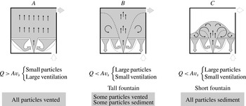
Figure 11. Schematic showing the three particle transport regimes.
It should be noted that since the cross-section of the tank is rectangular, the detailed flow pattern near the bounding walls in the lower layer will be different to that modelled by (3.5). However, motivated by the success of this model in describing the experiments of Zarrebini & Cardoso (Reference Zarrebini and Cardoso2000) and by the comparison of our experimental results with the predictions of the model, we assume that the use of (3.8) provides a leading-order criterion for the transition from the entrainment area to the sediment area in the lower layer. The equation is solved, using
 $r(y=0)=0$
as a boundary condition, to identify the maximum effective radius
$r(y=0)=0$
as a boundary condition, to identify the maximum effective radius
 $r$
at which a particle at a vertical distance
$r$
at which a particle at a vertical distance
 $y$
from the floor is entrained by the plume. For
$y$
from the floor is entrained by the plume. For
 $y=h_{i}$
, we obtain the critical entrainment area
$y=h_{i}$
, we obtain the critical entrainment area
 $A_{ent}$
at the level of the interface (figure 10
b):
$A_{ent}$
at the level of the interface (figure 10
b):
 $$\begin{eqnarray}{\rm\pi}r^{2}(h_{i})=A_{ent}=\frac{{\it\lambda}B^{1/3}h_{i}^{5/3}}{v_{s}}=\frac{Q}{v_{s}}.\end{eqnarray}$$
Equation (3.9) indicates that for a given settling speed
 $v_{s}$
and a given ventilation rate
$v_{s}$
and a given ventilation rate
 $Q$
, a fraction
$Q$
, a fraction
 $A_{ent}/A=Q/Av_{s}$
of all the particles which settle across the interface is entrained by the plume and re-suspended into the upper layer. The remaining particles,
$A_{ent}/A=Q/Av_{s}$
of all the particles which settle across the interface is entrained by the plume and re-suspended into the upper layer. The remaining particles,
 $1-Q/Av_{s}$
, sediment over the floor instead. When the critical area is equal to or larger than the floor area,
$1-Q/Av_{s}$
, sediment over the floor instead. When the critical area is equal to or larger than the floor area,
 $Q\geqslant Av_{s}$
, to leading order we expect all particles in the lower layer to be entrained by the plume.
$Q\geqslant Av_{s}$
, to leading order we expect all particles in the lower layer to be entrained by the plume.
3.1.3. Particle transport regimes
We combine (3.1)–(3.3) and (3.9) and obtain that the flux of particles vented from the space is given by
 $$\begin{eqnarray}P_{out}=P_{in}-C_{int}[Av_{s}-\min (Q,Av_{s})],\end{eqnarray}$$
while the flux of particles which sediment over the floor is given by
 $$\begin{eqnarray}P_{floor}=C_{int}[Av_{s}-\min (Q,Av_{s})].\end{eqnarray}$$
Equations (3.10) and (3.11) show that when the rate of ventilation of the space exceeds the critical level
 $Q_{crit}=Av_{s}$
, all particles are vented from the space through the high-level opening, and none sediments over the floor (see figure 11, particle transport regime A). This happens because for
$Q_{crit}=Av_{s}$
, all particles are vented from the space through the high-level opening, and none sediments over the floor (see figure 11, particle transport regime A). This happens because for
 $Q>Av_{s}$
, all the particles in the lower layer are entrained by the plume and suspended into the upper layer (cf. (3.9)). In this layer, the mean speed at which the ambient fluid rises towards the high-level vent,
$Q>Av_{s}$
, all the particles in the lower layer are entrained by the plume and suspended into the upper layer (cf. (3.9)). In this layer, the mean speed at which the ambient fluid rises towards the high-level vent,
 $Q/A$
, is larger than the speed at which particles settle,
$Q/A$
, is larger than the speed at which particles settle,
 $v_{s}$
. Hence, particles are advected to the top of the upper layer, and eventually vented from the space through the high-level opening.
$v_{s}$
. Hence, particles are advected to the top of the upper layer, and eventually vented from the space through the high-level opening.
For
 $Q<Av_{s}$
, however, some particles sediment over the floor as a result of the limited entrainment of the plume in the lower layer (cf. (3.9)). In this case, the number of particles vented from the space is controlled by the concentration at the level of the interface,
$Q<Av_{s}$
, however, some particles sediment over the floor as a result of the limited entrainment of the plume in the lower layer (cf. (3.9)). In this case, the number of particles vented from the space is controlled by the concentration at the level of the interface,
 $C_{int}$
, which in turn depends on the distribution of particles in the upper layer. We consider two bounding scenarios. When
$C_{int}$
, which in turn depends on the distribution of particles in the upper layer. We consider two bounding scenarios. When
 $Q<Av_{s}$
and the fountain in the upper layer reaches the top of the space,
$Q<Av_{s}$
and the fountain in the upper layer reaches the top of the space,
 $h_{f}>(H-h_{i})$
, the upper layer is well-mixed with a uniform concentration of particles (see figure 8). In this case, we expect that some particles will be vented from the space through the high-level opening, while some particles will sediment over the floor (see figure 11, particle transport regime B).
$h_{f}>(H-h_{i})$
, the upper layer is well-mixed with a uniform concentration of particles (see figure 8). In this case, we expect that some particles will be vented from the space through the high-level opening, while some particles will sediment over the floor (see figure 11, particle transport regime B).
However, when
 $Q<Av_{s}$
and the fountain in the upper layer is short,
$Q<Av_{s}$
and the fountain in the upper layer is short,
 $h_{f}<(H-h_{i})$
, particles are not transported to the top of the space by the fountain. Because of their large settling speed, particles are not advected to the top of the space by the mean motion of the fluid in the upper layer. Hence, we expect that none of the particles supplied to the space will be vented from it, and all of them will sediment over the floor at steady state (see figure 11, particle transport regime C).
$h_{f}<(H-h_{i})$
, particles are not transported to the top of the space by the fountain. Because of their large settling speed, particles are not advected to the top of the space by the mean motion of the fluid in the upper layer. Hence, we expect that none of the particles supplied to the space will be vented from it, and all of them will sediment over the floor at steady state (see figure 11, particle transport regime C).
In the next sections, we analyse each of these particle transport regimes separately, and we focus on the particle mass balance in the upper layer to quantify the number of particles extracted from the space,
 $P_{out}$
, and the concentration at the level of the interface,
$P_{out}$
, and the concentration at the level of the interface,
 $C_{int}$
. Based on the difference between the concentration of particles in the plume fluid and that in the upper layer fluid at the level of the interface, we calculate the height of the fountain in the upper layer, and determine the range of ventilation rates at which regimes B and C develop.
$C_{int}$
. Based on the difference between the concentration of particles in the plume fluid and that in the upper layer fluid at the level of the interface, we calculate the height of the fountain in the upper layer, and determine the range of ventilation rates at which regimes B and C develop.
3.1.4. Transport regime A
In the first transport regime, the ventilation flow rate exceeds the critical level
 $Q>Av_{s}$
(figure 11). We write the balance of the fluxes of particles in the upper layer at steady state (see figure 10
a):
$Q>Av_{s}$
(figure 11). We write the balance of the fluxes of particles in the upper layer at steady state (see figure 10
a):
 $$\begin{eqnarray}P_{out}+P_{set}=P_{in}+P_{ent}.\end{eqnarray}$$
In this regime, all particles in the lower layer are entrained by the plume:
 $$\begin{eqnarray}P_{set}=P_{ent}.\end{eqnarray}$$
A combination of (3.1), (3.12) and (3.13) shows that all particles are vented from the space through the high-level opening, and none sediments over the floor at steady state:
 $$\begin{eqnarray}P_{out}=P_{in},\quad P_{floor}=0.\end{eqnarray}$$
The concentration of particles suspended in the upper layer fluid is given by
 $$\begin{eqnarray}C_{int}=C_{out}=\frac{P_{in}}{Q},\end{eqnarray}$$
which results in a settling flux across the interface:
 $$\begin{eqnarray}P_{set}=\frac{Av_{s}}{Q}P_{in}.\end{eqnarray}$$
Since
 $Q/A>v_{s}$
, all the particles which settle across the interface from the upper layer into the lower layer are entrained by the plume, and the concentration of particles in the plume at the level of the interface is given by
$Q/A>v_{s}$
, all the particles which settle across the interface from the upper layer into the lower layer are entrained by the plume, and the concentration of particles in the plume at the level of the interface is given by
 $$\begin{eqnarray}C_{p,int}=\left(1+\frac{Av_{s}}{Q}\right)\frac{P_{in}}{Q}.\end{eqnarray}$$
We compare (3.15) and (3.17) and observe that in this first regime the plume fluid is more concentrated than the surrounding ambient fluid at the level of the interface. The concentration difference is given by
 $$\begin{eqnarray}{\rm\Delta}C=C_{p,int}-C_{int}=\frac{Av_{s}}{Q^{2}}P_{in}.\end{eqnarray}$$
3.1.5. Transport regime B
In regime B, particles are sufficiently large that some of them sediment over the floor at steady state. In the upper layer, the fountain reaches the top of the space and produces a uniform concentration of particles (see figure 11). The balance of the fluxes of particles in the upper layer at steady state is given by a combination of (3.9) and (3.12):
 $$\begin{eqnarray}C_{int}(Q+Av_{s})=P_{in}+\frac{Q}{Av_{s}}C_{int}Av_{s},\end{eqnarray}$$
from which we obtain
 $$\begin{eqnarray}C_{int}=C_{out}=\frac{P_{in}}{Av_{s}}.\end{eqnarray}$$
A combination of (3.10) and (3.11) and (3.20) gives the fraction of particles which are vented from the space through the high-level opening:
 $$\begin{eqnarray}P_{out}=\frac{Q}{Av_{s}}P_{in},\end{eqnarray}$$
and the fraction of particles which sediment over the floor:
 $$\begin{eqnarray}P_{floor}=\left(1-\frac{Q}{Av_{s}}\right)P_{in}.\end{eqnarray}$$
Equation (3.20) indicates that the flux of particles which settle across the interface equals the flux of particles supplied to the space:
 $$\begin{eqnarray}P_{set}=P_{in}.\end{eqnarray}$$
A fraction
 $Q/Av_{s}$
of these particles are entrained by the plume in the lower layer (cf. (3.9)). We combine (3.9), (3.20) and (3.23) to calculate the concentration of particles in the plume at the level of the interface:
$Q/Av_{s}$
of these particles are entrained by the plume in the lower layer (cf. (3.9)). We combine (3.9), (3.20) and (3.23) to calculate the concentration of particles in the plume at the level of the interface:
 $$\begin{eqnarray}C_{p,int}=\left(1+\frac{Q}{Av_{s}}\right)\frac{P_{in}}{Q}.\end{eqnarray}$$
We compare (3.20) and (3.24) and observe that the particle concentration in the plume is larger than that in the upper layer fluid at the level of the interface; the concentration difference is given by
 $$\begin{eqnarray}{\rm\Delta}C=C_{p,int}-C_{int}=\frac{P_{in}}{Q}.\end{eqnarray}$$
As a result of this concentration difference, the bulk density of the plume fluid is larger than that of the upper layer fluid at the level of the interface. The negative buoyancy flux of the plume is given by
 $$\begin{eqnarray}B_{p}=Q\,{\rm\Delta}C\,g\frac{{\it\rho}_{P}-{\it\rho}_{W}}{{\it\rho}_{W}},\end{eqnarray}$$
in which
 $g$
is the gravitational acceleration,
$g$
is the gravitational acceleration,
 ${\it\rho}_{P}$
is the density of the particles and
${\it\rho}_{P}$
is the density of the particles and
 ${\it\rho}_{W}$
is the density of the ambient fluid in the upper layer. The negative buoyancy
${\it\rho}_{W}$
is the density of the ambient fluid in the upper layer. The negative buoyancy
 $B_{p}$
controls the height of the fountain in the upper layer. Literature on turbulent fountains, including Turner (Reference Turner1966), Mizushina et al. (Reference Mizushina, Ogino, Takeuchi and Ikawa1982), Bloomfield & Kerr (Reference Bloomfield and Kerr1998, Reference Bloomfield and Kerr2000) and Burridge & Hunt (Reference Burridge and Hunt2012), indicates that the height of rise of a fountain,
$B_{p}$
controls the height of the fountain in the upper layer. Literature on turbulent fountains, including Turner (Reference Turner1966), Mizushina et al. (Reference Mizushina, Ogino, Takeuchi and Ikawa1982), Bloomfield & Kerr (Reference Bloomfield and Kerr1998, Reference Bloomfield and Kerr2000) and Burridge & Hunt (Reference Burridge and Hunt2012), indicates that the height of rise of a fountain,
 $h_{f}$
, is given by
$h_{f}$
, is given by
 $$\begin{eqnarray}h_{f}={\it\gamma}M^{3/4}B_{p}^{-1/2},\end{eqnarray}$$
in which
 $M$
is the momentum flux of the plume fluid at the interface:
$M$
is the momentum flux of the plume fluid at the interface:
 $$\begin{eqnarray}M=\frac{Q^{2}}{{\rm\pi}r_{p}^{2}},\end{eqnarray}$$
and
 ${\it\gamma}$
is a constant of order 1. In a set of experiments on turbulent fountains, Bloomfield & Kerr (Reference Bloomfield and Kerr2000) measured
${\it\gamma}$
is a constant of order 1. In a set of experiments on turbulent fountains, Bloomfield & Kerr (Reference Bloomfield and Kerr2000) measured
 ${\it\gamma}=1.70\pm 0.17$
; similar results were obtained by the other researchers cited above. To determine the range of ventilation rates at which regime B develops, we compare the height of the fountain with the height of the upper layer,
${\it\gamma}=1.70\pm 0.17$
; similar results were obtained by the other researchers cited above. To determine the range of ventilation rates at which regime B develops, we compare the height of the fountain with the height of the upper layer,
 $H-h_{i}$
. Using a combination of (2.1), (3.25)–(3.28), we obtain that the fountain reaches the top of the space when
$H-h_{i}$
. Using a combination of (2.1), (3.25)–(3.28), we obtain that the fountain reaches the top of the space when
 $$\begin{eqnarray}Q>{\it\gamma}^{-2/3}A_{p}^{1/2}B_{p}^{1/3}(H-h_{i})^{2/3},\end{eqnarray}$$
in which
 $$\begin{eqnarray}A_{p}={\rm\pi}\left({\textstyle \frac{6}{5}}{\it\alpha}h_{i}\right)^{2}\end{eqnarray}$$
is the cross-sectional area of the plume at the level of the interface. Equation (3.29) indicates that the fountain reaches the top of the upper layer when the ventilation rate
 $Q$
is sufficiently large. A larger flow rate is required when the enclosure is tall (large
$Q$
is sufficiently large. A larger flow rate is required when the enclosure is tall (large
 $H$
), or when a large number of particles are supplied to the space (resulting in a large buoyancy flux
$H$
), or when a large number of particles are supplied to the space (resulting in a large buoyancy flux
 $B_{p}$
, cf. (3.25) and (3.26)).
$B_{p}$
, cf. (3.25) and (3.26)).
3.1.6. Transport regime C
In regime C (figure 11), the fountain in the upper layer does not reach the top of the space. Hence, particles are not transported to the top of the upper layer, where the outlet vent is located. Consequently, all particles sediment over the floor at steady state:
 $$\begin{eqnarray}P_{out}=0,\quad P_{floor}=P_{in}.\end{eqnarray}$$
We combine (3.9), (3.12) and (3.31a,b ) to write the balance of the fluxes of particles in the upper layer at steady state:
 $$\begin{eqnarray}C_{int}Av_{s}=P_{in}+\frac{Q}{Av_{s}}C_{int}Av_{s}\end{eqnarray}$$
from which we obtain
 $$\begin{eqnarray}C_{int}=\frac{P_{in}}{Av_{s}-Q}.\end{eqnarray}$$
At this concentration particles settle from the upper layer into the lower layer across the interface. A fraction
 $Q/Av_{s}$
of them is entrained by the plume (cf. (3.9)). Consequently, the concentration of particles in the plume fluid at the level of the interface is given by
$Q/Av_{s}$
of them is entrained by the plume (cf. (3.9)). Consequently, the concentration of particles in the plume fluid at the level of the interface is given by
 $$\begin{eqnarray}C_{p,int}=\frac{P_{in}}{Q}+\frac{P_{in}}{Av_{s}-Q}.\end{eqnarray}$$
We compare (3.33) and (3.34) and observe that the particle concentration in the plume is larger than that in the upper layer fluid at the level of the interface. The concentration difference,
 ${\rm\Delta}C$
, and the negative buoyancy flux of the fountain fluid at the level of the interface,
${\rm\Delta}C$
, and the negative buoyancy flux of the fountain fluid at the level of the interface,
 $B_{p}$
, are the same as in regime B, and are given by (3.25) and (3.26) respectively. To determine the range of ventilation rates at which regime C develops, we compare the height of the fountain with the height of the upper layer. We predict that the fountain does not reach the top of the space if
$B_{p}$
, are the same as in regime B, and are given by (3.25) and (3.26) respectively. To determine the range of ventilation rates at which regime C develops, we compare the height of the fountain with the height of the upper layer. We predict that the fountain does not reach the top of the space if
 $$\begin{eqnarray}Q<{\it\gamma}^{-2/3}A_{p}^{1/2}B_{p}^{1/3}(H-h_{i})^{2/3}.\end{eqnarray}$$
The critical flow rate at which the height of the fountain equals the height of the room given by (3.35) is identical to that given by (3.29), showing that the models developed in §§ 3.1.5 and 3.1.6 are self-consistent.
3.1.7. Uniform concentration of particles at the level of the two-layer density interface
Equations (3.26) and (3.28) are used to test our initial assumption that the concentration of particles in the lower part of the upper layer,
 $C_{int}$
, is uniform across the width of the tank (cf. § 3.1.2). In regime B the upper layer is well-mixed by the fountain and therefore the concentration of particles at the level of the interface is uniform (cf. § 3.1.5). In regime C, however, the upper layer is stratified with particles. In that case, the fountain fluid reaches a maximum height in the upper layer,
$C_{int}$
, is uniform across the width of the tank (cf. § 3.1.2). In regime B the upper layer is well-mixed by the fountain and therefore the concentration of particles at the level of the interface is uniform (cf. § 3.1.5). In regime C, however, the upper layer is stratified with particles. In that case, the fountain fluid reaches a maximum height in the upper layer,
 $h_{f}$
, and then falls towards the two-layer density interface. On reaching the interface, the fountain fluid spreads radially over the interface and forms a gravity current (see figure 12). The particle volume fraction in the current,
$h_{f}$
, and then falls towards the two-layer density interface. On reaching the interface, the fountain fluid spreads radially over the interface and forms a gravity current (see figure 12). The particle volume fraction in the current,
 ${\it\phi}$
, decreases with radius as a result of gravitational settling of particles across the interface (Woods Reference Woods2010):
${\it\phi}$
, decreases with radius as a result of gravitational settling of particles across the interface (Woods Reference Woods2010):
 $$\begin{eqnarray}\frac{\text{d}}{\text{d}r}(ruh{\it\phi})=-rv_{s}{\it\phi},\end{eqnarray}$$
in which
 $u$
is the radial speed of the current,
$u$
is the radial speed of the current,
 $h$
is the depth of the current and
$h$
is the depth of the current and
 $r$
is the radial distance from the vertical axis of the fountain (figure 12). We solve (3.36) and obtain that, as particles settle out of the current across the interface, the mass of particles in the current decays with radius as
$r$
is the radial distance from the vertical axis of the fountain (figure 12). We solve (3.36) and obtain that, as particles settle out of the current across the interface, the mass of particles in the current decays with radius as
 $$\begin{eqnarray}{\it\phi}(r)={\it\phi}_{0}\exp \left[-\frac{2{\rm\pi}v_{s}}{Q_{f}}\left(r^{2}-r_{0}^{2}\right)\right],\end{eqnarray}$$
in which
 ${\it\phi}_{0}$
is the particle volume fraction in the descending fountain fluid at the level of the interface,
${\it\phi}_{0}$
is the particle volume fraction in the descending fountain fluid at the level of the interface,
 $r_{0}$
is the outer radius of the fountain at the level of the interface, and
$r_{0}$
is the outer radius of the fountain at the level of the interface, and
 $$\begin{eqnarray}Q_{f}=2{\rm\pi}ruh\end{eqnarray}$$
is the volume flux of the fountain at the level of the interface.
 $Q_{f}$
is controlled by the momentum flux and the buoyancy flux of the fountain fluid at the level of the interface:
$Q_{f}$
is controlled by the momentum flux and the buoyancy flux of the fountain fluid at the level of the interface:
 $$\begin{eqnarray}Q_{f}=k\frac{M^{5/4}}{B_{p}^{1/2}},\end{eqnarray}$$
in which
 $k$
is a constant of order 1 (cf. Mizushina et al.
Reference Mizushina, Ogino, Takeuchi and Ikawa1982; Bloomfield & Kerr Reference Bloomfield and Kerr2000). We combine (3.37) and (3.39) and obtain the length scale for a change in the concentration of particles in the current as a result of the particle fallout:
$k$
is a constant of order 1 (cf. Mizushina et al.
Reference Mizushina, Ogino, Takeuchi and Ikawa1982; Bloomfield & Kerr Reference Bloomfield and Kerr2000). We combine (3.37) and (3.39) and obtain the length scale for a change in the concentration of particles in the current as a result of the particle fallout:
 $$\begin{eqnarray}L=\frac{M^{5/8}}{v_{s}^{1/2}B_{p}^{1/4}}.\end{eqnarray}$$

Figure 12. Gravity current at the base of the upper layer in regime C.
For each of the experiments plotted in figure 9(b), we calculate
 $L$
using (3.26) and (3.28). We then compare
$L$
using (3.26) and (3.28). We then compare
 $L$
with the distance between the vertical axis of the fountain and the walls of the tank,
$L$
with the distance between the vertical axis of the fountain and the walls of the tank,
 $0.5\sqrt{A}$
. Table 1 shows that
$0.5\sqrt{A}$
. Table 1 shows that
 $L\gg 0.5\sqrt{A}$
in all the experiments in which small particles of a mean diameter
$L\gg 0.5\sqrt{A}$
in all the experiments in which small particles of a mean diameter
 $18.3~{\rm\mu}\text{m}$
are used. Consequently, we do not expect the concentration of particles in the current at the base of the upper layer to change significantly across the width of the tank. This is consistent with the experimental results illustrated by figures 6 and 7, and supports our initial assumption that
$18.3~{\rm\mu}\text{m}$
are used. Consequently, we do not expect the concentration of particles in the current at the base of the upper layer to change significantly across the width of the tank. This is consistent with the experimental results illustrated by figures 6 and 7, and supports our initial assumption that
 $C_{int}$
is uniform across the width of the tank.
$C_{int}$
is uniform across the width of the tank.
3.2. Polydisperse suspension of particles
In this section, we extend the model developed in § 3.1 to describe the transport of a polydisperse suspension of particles, i.e. a suspension in which there are particles of different sizes. For a given ventilation rate
 $Q$
and a given floor area
$Q$
and a given floor area
 $A$
, we define
$A$
, we define
 $D_{c}$
as the critical diameter at which the settling speed of a particle equals the mean speed at which the ambient fluid rises through the upper layer towards the high-level vent,
$D_{c}$
as the critical diameter at which the settling speed of a particle equals the mean speed at which the ambient fluid rises through the upper layer towards the high-level vent,
 $Q/A$
. For the small particles used in this study, Stokes law describes the settling speed of the particles and leads to the prediction that
$Q/A$
. For the small particles used in this study, Stokes law describes the settling speed of the particles and leads to the prediction that
 $D_{c}$
is given by
$D_{c}$
is given by
 $$\begin{eqnarray}D_{c}=\left[\frac{18{\it\mu}}{({\it\rho}_{P}-{\it\rho}_{W})g}\frac{Q}{A}\right]^{1/2},\end{eqnarray}$$
in which
 ${\it\mu}$
is the dynamic viscosity of the ambient fluid. A polydisperse suspension will contain a certain number of particles whose diameter is smaller than
${\it\mu}$
is the dynamic viscosity of the ambient fluid. A polydisperse suspension will contain a certain number of particles whose diameter is smaller than
 $D_{c}$
: for convenience, from now on we will refer to these particles as the small particles in the suspension. The suspension will also contain a certain number of particles whose diameter is larger than
$D_{c}$
: for convenience, from now on we will refer to these particles as the small particles in the suspension. The suspension will also contain a certain number of particles whose diameter is larger than
 $D_{c}$
. We will refer to these particles as the large particles in the suspension.
$D_{c}$
. We will refer to these particles as the large particles in the suspension.
For different rates of ventilation of the space and different heights of the fountain in the upper layer, the transport of the small particles through the space may be different to that of the large particles. Figure 13 shows that four transport regimes can develop in the system.

Figure 13. Schematic showing the particle transport regimes for polydisperse suspensions.
For
 $Q>Av_{s,max}$
, the suspension only contains small particles, which are entrained in the lower layer and advected upwards through the upper layer. We denote this first regime
$Q>Av_{s,max}$
, the suspension only contains small particles, which are entrained in the lower layer and advected upwards through the upper layer. We denote this first regime
 ${\it\alpha}$
. In this regime, all particles are vented from the space, and none sediments over the floor, analogous to regime A in the monodisperse model described in § 3.1.4 and illustrated by figure 11.
${\it\alpha}$
. In this regime, all particles are vented from the space, and none sediments over the floor, analogous to regime A in the monodisperse model described in § 3.1.4 and illustrated by figure 11.
For
 $Q<Av_{s,max}$
, however, the suspension contains some large particles, which can sediment over the floor. The number of large particles which are vented out of the space depends on whether the upper layer is well-mixed or stratified. When the fountain reaches the top of the space and produces a well-mixed upper layer, regime
$Q<Av_{s,max}$
, however, the suspension contains some large particles, which can sediment over the floor. The number of large particles which are vented out of the space depends on whether the upper layer is well-mixed or stratified. When the fountain reaches the top of the space and produces a well-mixed upper layer, regime
 ${\it\beta}1$
develops (figure 13). In this regime, all the small particles are vented from the space through the high-level opening, because none of them can sediment over the floor due to the plume entrainment in the lower layer. As for the large particles, some of them are vented from the space at a high level, while the remaining particles sediment over the floor (compare with regime B in the monodisperse model described in § 3.1.5 and illustrated by figure 11).
${\it\beta}1$
develops (figure 13). In this regime, all the small particles are vented from the space through the high-level opening, because none of them can sediment over the floor due to the plume entrainment in the lower layer. As for the large particles, some of them are vented from the space at a high level, while the remaining particles sediment over the floor (compare with regime B in the monodisperse model described in § 3.1.5 and illustrated by figure 11).
When the fountain in the upper layer does not reach the top of the space, regime
 ${\it\beta}2$
develops instead. In this regime, small particles are advected to the top of the space and vented through the high-level opening. Large particles, however, are not transported to the top of the space, and sediment over the floor.
${\it\beta}2$
develops instead. In this regime, small particles are advected to the top of the space and vented through the high-level opening. Large particles, however, are not transported to the top of the space, and sediment over the floor.
When the rate of ventilation of the space is particularly weak,
 $Q<Av_{s,min}$
, the polydisperse suspension contains only particles which are sufficiently large that they fall through the upper layer fluid. In this case, regime
$Q<Av_{s,min}$
, the polydisperse suspension contains only particles which are sufficiently large that they fall through the upper layer fluid. In this case, regime
 ${\it\gamma}$
develops (figure 13), in which all particles sediment over the floor and none is vented from the space, analogous to regime C in the monodisperse model described in § 3.1.6 and illustrated by figure 11.
${\it\gamma}$
develops (figure 13), in which all particles sediment over the floor and none is vented from the space, analogous to regime C in the monodisperse model described in § 3.1.6 and illustrated by figure 11.
When a polydisperse suspension of particles is ventilated in modes
 ${\it\alpha}$
or
${\it\alpha}$
or
 ${\it\gamma}$
, the models developed in §§ 3.1.4 and 3.1.6 can be used to quantify the fluxes of particles transported through the space. In the next sections, we analyse regimes
${\it\gamma}$
, the models developed in §§ 3.1.4 and 3.1.6 can be used to quantify the fluxes of particles transported through the space. In the next sections, we analyse regimes
 ${\it\beta}$
1 and
${\it\beta}$
1 and
 ${\it\beta}$
2, and we quantify the number of particles extracted from the space,
${\it\beta}$
2, and we quantify the number of particles extracted from the space,
 $P_{out}$
, and the concentration at the level of the interface,
$P_{out}$
, and the concentration at the level of the interface,
 $C_{int}$
, in each regime. These models will be tested in § 3.3 by comparing the model predictions with the results of the experiments described in § 2.2.
$C_{int}$
, in each regime. These models will be tested in § 3.3 by comparing the model predictions with the results of the experiments described in § 2.2.
3.2.1. Transport regime
 ${\it\beta}1$

We first consider a space in which the fountain in the upper layer reaches the top of the space and produces a well-mixed distribution of particles above the two-layer density interface. A polydisperse suspension contains a certain number of small particles. We denote the volume fraction of the small particles in the suspension by
 ${\it\Phi}$
:
${\it\Phi}$
:
 $$\begin{eqnarray}{\it\Phi}=\frac{\displaystyle \int _{0}^{D_{c}}C(x)\;x^{3}\,\text{d}x}{\displaystyle \int _{0}^{\infty }C(x)\;x^{3}\,\text{d}x},\end{eqnarray}$$
and their weighted mean settling velocity by
 $\bar{v}_{s,small}$
:
$\bar{v}_{s,small}$
:
 $$\begin{eqnarray}\bar{v}_{s,small}=\frac{\displaystyle \int _{0}^{D_{c}}C(x)v_{s}(x)\,\text{d}x}{\displaystyle \int _{0}^{D_{c}}C(x)\,\text{d}x},\end{eqnarray}$$
where
 $D_{c}$
is defined by (3.41). The suspension also contains some large particles: the volume fraction of these particles is given by
$D_{c}$
is defined by (3.41). The suspension also contains some large particles: the volume fraction of these particles is given by
 $(1-{\it\Phi})$
, and their weighted mean settling velocity is denoted by
$(1-{\it\Phi})$
, and their weighted mean settling velocity is denoted by
 $\bar{v}_{s,large}$
:
$\bar{v}_{s,large}$
:
 $$\begin{eqnarray}\bar{v}_{s,large}=\frac{\displaystyle \int _{D_{c}}^{\infty }C(x)v_{s}(x)\,\text{d}x}{\displaystyle \int _{D_{c}}^{\infty }C(x)\,\text{d}x}.\end{eqnarray}$$
The flux of particles vented from the space through the high-level opening includes all the small particles (cf. (3.14)) and a fraction of the large ones (given by (3.21)):
 $$\begin{eqnarray}P_{out}={\it\Phi}P_{in}+(1-{\it\Phi})\frac{Q}{A\bar{v}_{s,large}}P_{in}.\end{eqnarray}$$
The remaining large particles sediment over the floor, as described by (3.22):
 $$\begin{eqnarray}P_{floor}=(1-{\it\Phi})\left(1-\frac{Q}{A\bar{v}_{s,large}}\right)P_{in}.\end{eqnarray}$$
To calculate the concentration in the upper layer, we combine (3.15) and (3.20) and obtain
 $$\begin{eqnarray}C_{int}=C_{out}={\it\Phi}\frac{P_{in}}{Q}+(1-{\it\Phi})\frac{P_{in}}{A\bar{v}_{s,large}}.\end{eqnarray}$$
To calculate the difference between the concentration of particles in the plume fluid and that in the upper layer fluid at the level of the interface we combine (3.18) and (3.25) and obtain
 $$\begin{eqnarray}{\rm\Delta}C=\frac{P_{in}}{Q}\left[1-{\it\Phi}\left(1-\frac{A\bar{v}_{s,small}}{Q}\right)\right].\end{eqnarray}$$
Based on the concentration difference
 ${\rm\Delta}C$
, we calculate the negative buoyancy flux of the fountain fluid at the level of the interface,
${\rm\Delta}C$
, we calculate the negative buoyancy flux of the fountain fluid at the level of the interface,
 $B_{p}$
, which is given by (3.26). The flux controls the height of the fountain in the upper layer, as described by (3.27). The criterion for the fountain to reach the top of the space is given by (3.29).
$B_{p}$
, which is given by (3.26). The flux controls the height of the fountain in the upper layer, as described by (3.27). The criterion for the fountain to reach the top of the space is given by (3.29).
3.2.2. Transport regime
${\it\beta}2$

We now consider the case of a weaker fountain which does not reach the top of the space (regime
 ${\it\beta}2$
in figure 13). In this case, we expect the small particles to be advected to the top of the space and vented to the exterior through the high-level opening:
${\it\beta}2$
in figure 13). In this case, we expect the small particles to be advected to the top of the space and vented to the exterior through the high-level opening:
 $$\begin{eqnarray}P_{out}={\it\Phi}P_{in}.\end{eqnarray}$$
The speed at which the large particles settle through the ambient fluid exceeds the mean speed at which the fluid rises through the upper layer; for this reason, we do not expect the large particles to be advected to the top of the space. Furthermore, in regime
 ${\it\beta}2$
the large particles are not transported to the top of the space by the fountain. As a result, we do not expect any of the large particles to reach the high-level vent, and so we assume that none is vented to the exterior and all sediment over the floor:
${\it\beta}2$
the large particles are not transported to the top of the space by the fountain. As a result, we do not expect any of the large particles to reach the high-level vent, and so we assume that none is vented to the exterior and all sediment over the floor:
 $$\begin{eqnarray}P_{floor}=(1-{\it\Phi})P_{in}.\end{eqnarray}$$
The concentration of the upper layer fluid at the level of the interface is given by a combination of (3.15) and (3.33):
 $$\begin{eqnarray}C_{int}={\it\Phi}\frac{P_{in}}{Q}+(1-{\it\Phi})\frac{P_{in}}{A\bar{v}_{s,large}-Q}.\end{eqnarray}$$
The difference between the concentration of particles in the plume fluid and that in the upper layer fluid at the level of the interface,
 ${\rm\Delta}C$
, is the same as in regime
${\rm\Delta}C$
, is the same as in regime
 ${\it\beta}1$
, and is given by (3.48). Consequently, the negative buoyancy flux of the fountain fluid at the level of the interface,
${\it\beta}1$
, and is given by (3.48). Consequently, the negative buoyancy flux of the fountain fluid at the level of the interface,
 $B_{p}$
, and the height of the fountain in the upper layer,
$B_{p}$
, and the height of the fountain in the upper layer,
 $h_{f}$
, can be calculated using the same equations listed in § 3.2.1. The criterion for the fountain to be short in the upper layer is given by (3.35).
$h_{f}$
, can be calculated using the same equations listed in § 3.2.1. The criterion for the fountain to be short in the upper layer is given by (3.35).
3.3. Testing the model
In this section, we test the model developed in §§ 3.1 and 3.2 by comparing model predictions with experimental results.
For a range of different experiments, in figure 14 we compare the fountain heights which we measured during the experiments with the model predictions given by (3.27). Results are plotted in dimensionless form by scaling the height of the fountain by the height of the upper layer. In plotting the horizontal axis of figure 14, we use a combination of (3.26), (3.27) and (3.48) to calculate the predicted fountain height. We also use (2.1) to calculate the predicted height of the upper layer,
 $H-h_{i}$
. The figure shows that in some experiments the fountain has sufficient momentum that it reaches the top of the tank (diamonds on the right-hand side). In other experiments, however, the fountain does not reach the top of the space (circles on the left-hand side). Experimental results agree with model predictions using the value
$H-h_{i}$
. The figure shows that in some experiments the fountain has sufficient momentum that it reaches the top of the tank (diamonds on the right-hand side). In other experiments, however, the fountain does not reach the top of the space (circles on the left-hand side). Experimental results agree with model predictions using the value
 ${\it\gamma}=1.55\pm 0.10$
(cf. (3.27)). This value of
${\it\gamma}=1.55\pm 0.10$
(cf. (3.27)). This value of
 ${\it\gamma}$
is compatible with the range of values given by Bloomfield & Kerr (Reference Bloomfield and Kerr2000). This suggests that the model developed in § 3.2 provides an accurate prediction of the negative buoyancy of the plume fluid at the level of the interface,
${\it\gamma}$
is compatible with the range of values given by Bloomfield & Kerr (Reference Bloomfield and Kerr2000). This suggests that the model developed in § 3.2 provides an accurate prediction of the negative buoyancy of the plume fluid at the level of the interface,
 $B_{p}$
.
$B_{p}$
.

Figure 14. Height of the particle-laden fountain relative to the height of the upper layer. On the horizontal axis we plot the predictions of the model developed in § 3, while on the vertical axis we plot the experimental outcomes (cf. table 1, the figure includes the results of the experiments with
 $A=0.0625~\text{m}^{2}$
). In some experiments the height of the fountain exceeds that of the upper layer (diamonds). When, however, the height of the fountain is smaller than the height of the layer (circles), we obtain
$A=0.0625~\text{m}^{2}$
). In some experiments the height of the fountain exceeds that of the upper layer (diamonds). When, however, the height of the fountain is smaller than the height of the layer (circles), we obtain
 ${\it\gamma}=1.55\pm 0.10$
.
${\it\gamma}=1.55\pm 0.10$
.
Figure 15(a) shows how the fraction of the particle flux which is vented from the space through the high-level opening,
 $P_{out}/P_{in}$
, changes when
$P_{out}/P_{in}$
, changes when
 $Q/A\bar{v}_{s}$
is changed. In the figure, a thick grey line has been plotted using (3.45): this line shows the fraction of particles vented from the space when the fountain fluid reaches the top of the upper layer (regime
$Q/A\bar{v}_{s}$
is changed. In the figure, a thick grey line has been plotted using (3.45): this line shows the fraction of particles vented from the space when the fountain fluid reaches the top of the upper layer (regime
 ${\it\beta}1$
). A thick black line has been plotted using (3.49) and illustrates the fraction of particles vented from the space when the fountain fluid does not reach the top of the upper layer (regime
${\it\beta}1$
). A thick black line has been plotted using (3.49) and illustrates the fraction of particles vented from the space when the fountain fluid does not reach the top of the upper layer (regime
 ${\it\beta}2$
). In the figure, there are solid and dashed sections of these lines. The solid part each line is designed to illustrate the region in which that model applies, based on
${\it\beta}2$
). In the figure, there are solid and dashed sections of these lines. The solid part each line is designed to illustrate the region in which that model applies, based on
 $h_{f}\gtrless (H-h_{i})$
. The figure shows that the grey line fits well the outcomes of those experiments in which the fountain is tall and the concentration in the upper layer is uniform (circles on the right-hand side of figure 15(a), see figures 6 and 8). The black line, however, fits well the outcomes of those experiments in which the fountain is short and does not reach the ceiling of the space (circles on the left-hand side of figure 15
a). The transition between the stratified scenario and the well-mixed scenario is smooth: for
$h_{f}\gtrless (H-h_{i})$
. The figure shows that the grey line fits well the outcomes of those experiments in which the fountain is tall and the concentration in the upper layer is uniform (circles on the right-hand side of figure 15(a), see figures 6 and 8). The black line, however, fits well the outcomes of those experiments in which the fountain is short and does not reach the ceiling of the space (circles on the left-hand side of figure 15
a). The transition between the stratified scenario and the well-mixed scenario is smooth: for
 $1.2<Q/A\bar{v}_{s}<1.4$
, the fountain is strong enough to lift a certain number of large particles to the level of the outlet vent, but not sufficiently strong to produce a perfectly well-mixed environment in the upper layer. For these experiments, the fraction of particles removed through the high-level vent is larger than
$1.2<Q/A\bar{v}_{s}<1.4$
, the fountain is strong enough to lift a certain number of large particles to the level of the outlet vent, but not sufficiently strong to produce a perfectly well-mixed environment in the upper layer. For these experiments, the fraction of particles removed through the high-level vent is larger than
 ${\it\Phi}$
(regime
${\it\Phi}$
(regime
 ${\it\beta}2$
, cf. (3.49)), but smaller than
${\it\beta}2$
, cf. (3.49)), but smaller than
 ${\it\Phi}+(1-{\it\Phi})Q/A\bar{v}_{s,large}$
(regime
${\it\Phi}+(1-{\it\Phi})Q/A\bar{v}_{s,large}$
(regime
 ${\it\beta}1$
, cf. (3.45)).
${\it\beta}1$
, cf. (3.45)).

Figure 15. Comparison of model predictions (lines) with experimental results (symbols): (a) fraction of the particle flux which is vented from the tank through the high-level opening,
 $P_{out}/P_{in}$
; (b) concentration of particles at the level of the interface relative to the concentration of particles the plume fluid at the source,
$P_{out}/P_{in}$
; (b) concentration of particles at the level of the interface relative to the concentration of particles the plume fluid at the source,
 $C_{int}/C_{in}$
.
$C_{int}/C_{in}$
.
A thin dot-dashed line in figure 15(a) illustrates the prediction of a model which assumes that both the lower and the upper layer are well-mixed with a uniform concentration of particles (Bolster & Linden Reference Bolster and Linden2009a ). This model overestimates the number of particles vented from the space when the fountain does not reach the top, and the upper layer is stratified with particles (circles on the left-hand side of figure 15 a). For large ventilation flow rates, the model underestimates the number of particles entrained by the plume in the lower layer, and consequently underestimates the number of particles which are vented from the space at steady state (circles on the right-hand side of figure 15 a).
Figure 15(b) shows how the concentration in the lower part of the upper layer changes when
 $Q/A\bar{v}_{s}$
is changed. In plotting this figure,
$Q/A\bar{v}_{s}$
is changed. In plotting this figure,
 $C_{int}$
is scaled by the concentration of particles in the plume fluid at the source. As in figure 15(a), a grey line has been plotted in figure 15(b) using (3.47) to illustrate the prediction of the tall-fountain model (regime
$C_{int}$
is scaled by the concentration of particles in the plume fluid at the source. As in figure 15(a), a grey line has been plotted in figure 15(b) using (3.47) to illustrate the prediction of the tall-fountain model (regime
 ${\it\beta}1$
). A black line has been plotted using (3.51) to illustrate the prediction of the short-fountain model (regime
${\it\beta}1$
). A black line has been plotted using (3.51) to illustrate the prediction of the short-fountain model (regime
 ${\it\beta}2$
). Figure 15(b) shows that the concentration at the level of the interface is large when the ventilation flow rate
${\it\beta}2$
). Figure 15(b) shows that the concentration at the level of the interface is large when the ventilation flow rate
 $Q$
is sufficiently small that the fountain does not reach the top of the upper layer (short-fountain model, black line), but also large enough that a significant number of particles are entrained in the lower layer and recirculated across the interface. For small values of
$Q$
is sufficiently small that the fountain does not reach the top of the upper layer (short-fountain model, black line), but also large enough that a significant number of particles are entrained in the lower layer and recirculated across the interface. For small values of
 $Q$
, a limited number of particles are entrained by the plume and re-suspended (cf. (3.9)): this reduces the concentration at the level of the interface,
$Q$
, a limited number of particles are entrained by the plume and re-suspended (cf. (3.9)): this reduces the concentration at the level of the interface,
 $C_{int}$
, and the residence time of the particles within the space. For large values of
$C_{int}$
, and the residence time of the particles within the space. For large values of
 $Q$
, the fraction of particles whose settling speed exceeds the background flow speed,
$Q$
, the fraction of particles whose settling speed exceeds the background flow speed,
 $1-{\it\Phi}$
, is reduced. Hence, the well-mixed model and the stratified model predict similar concentrations at the interface (cf. (3.47) and (3.51) respectively).
$1-{\it\Phi}$
, is reduced. Hence, the well-mixed model and the stratified model predict similar concentrations at the interface (cf. (3.47) and (3.51) respectively).
The thin dot-dashed line in figure 15(b) shows the prediction of a model which assumes that both the lower and the upper layer are well-mixed with a uniform concentration of particles. As noted above, this model tends to underestimate the flux of particles which are entrained by the plume in the lower layer. As a result, it also underestimates the number of particles which are continuously recirculated and suspended in the fluid at the level of the interface.
Figures 14 and 15 show that there is reasonable agreement of the two models developed in §§ 3.2.1 and 3.2.2 with the experimental data, and that the transition from one model to the other also seems to describe the transition in the data to leading order. Some of the difference between the experimental data and the predictions of the models may arise from the rectangular geometry of the space, while our models assume the entrainment flow in the lower layer to be axisymmetric (cf. § 3.1.2). However, the models appear to provide a leading-order description of the sedimentation and re-entrainment of particles in the lower layer. This results in a good quantitative prediction of the experimental data in the different regimes, in terms of both the fountain height and the particle concentration and particle flux being vented from the space.
4. Discussion and conclusions
We have explored the ventilation of an enclosed space in which a plume is generated by a localised source of buoyancy. The plume is contaminated with particles which settle through the surrounding fluid. A ventilation flow of uncontaminated fluid is supplied into the space at a low level, and an equivalent amount of fluid is extracted from the space at a high level. At steady state, a two-layer density stratification develops in the space. Using an image-processing technique, we have observed that the particle-laden plume rises through the lower layer while entraining fluid and particles from the surrounding environment. On reaching the density interface, the plume fluid becomes negatively buoyant relative to the ambient fluid in the upper layer. As a result, a fountain is formed in the upper layer: the height of this fountain is controlled by the momentum and the concentration of the plume fluid at the interface level. We have observed that the concentration profile in the upper layer is controlled by the height of the fountain relative to the height of the space. Fountains with sufficient momentum reach the top of the space and spread over the ceiling, leading to a well-mixed environment with a uniform concentration of particles above the interface. Shorter fountains, however, result in a stratified upper layer, in which the concentration at the level of the interface is higher than that at the level of the outlet vent. In this case, the concentration at the level of the interface is uniform across the width of the space, provided that the fountain flow rate is large and the settling speed of the particles is small (cf. (3.40)).
We have identified three particle transport regimes, which are controlled by: (i) the rate of ventilation of the space,
 $Q$
; (ii) the settling speed of the particles,
$Q$
; (ii) the settling speed of the particles,
 $v_{s}$
; and (iii) the floor area and the height of the space,
$v_{s}$
; and (iii) the floor area and the height of the space,
 $A$
and
$A$
and
 $H$
respectively. We have shown that when the rate of ventilation of the space is larger than the critical level,
$H$
respectively. We have shown that when the rate of ventilation of the space is larger than the critical level,
 $Q>Av_{s}$
(regime A), all particles in the lower layer are entrained by the plume and suspended into the upper layer before they can reach the floor and sediment. In the upper layer, particles are advected upwards by the mean motion of the fluid, so they all reach the top of the space, irrespective of the fountain height and of the room height. Eventually, all particles are vented to the exterior through the high-level opening (cf. (3.10)). For
$Q>Av_{s}$
(regime A), all particles in the lower layer are entrained by the plume and suspended into the upper layer before they can reach the floor and sediment. In the upper layer, particles are advected upwards by the mean motion of the fluid, so they all reach the top of the space, irrespective of the fountain height and of the room height. Eventually, all particles are vented to the exterior through the high-level opening (cf. (3.10)). For
 $Q>Av_{s}$
, an increase in the ventilation flow rate
$Q>Av_{s}$
, an increase in the ventilation flow rate
 $Q$
is conducive to a reduction in the concentration of particles in the upper layer (cf. (3.15)).
$Q$
is conducive to a reduction in the concentration of particles in the upper layer (cf. (3.15)).
When the floor area is sufficiently large that the rate of ventilation is smaller than the critical level,
 $Q<Av_{s}$
, however, particles settle faster than the ambient fluid rises through the upper layer. In this case, particles reach the top of the space only when the fountain reaches the top of the space and produces a well-mixed environment above the interface (regime B). This happens when the height of the fountain equals or exceeds the room height
$Q<Av_{s}$
, however, particles settle faster than the ambient fluid rises through the upper layer. In this case, particles reach the top of the space only when the fountain reaches the top of the space and produces a well-mixed environment above the interface (regime B). This happens when the height of the fountain equals or exceeds the room height
 $H$
(cf. (3.29)). In this case, a fraction
$H$
(cf. (3.29)). In this case, a fraction
 $Q/Av_{s}$
of the total number of particles supplied to the space are vented to the exterior (cf. (3.21)), while the remaining particles sediment over the floor. In regime B, the concentration of particles in the well-mixed upper layer is not controlled by the flow rate
$Q/Av_{s}$
of the total number of particles supplied to the space are vented to the exterior (cf. (3.21)), while the remaining particles sediment over the floor. In regime B, the concentration of particles in the well-mixed upper layer is not controlled by the flow rate
 $Q$
(cf. (3.20)). This happens because an increase in the rate of ventilation of the space,
$Q$
(cf. (3.20)). This happens because an increase in the rate of ventilation of the space,
 $Q$
, results in more particles being vented from the upper layer,
$Q$
, results in more particles being vented from the upper layer,
 $P_{out}$
, but also in more particles being entrained and re-suspended by the plume in the lower layer,
$P_{out}$
, but also in more particles being entrained and re-suspended by the plume in the lower layer,
 $P_{ent}$
. These two effects are balanced, so that
$P_{ent}$
. These two effects are balanced, so that
 $C_{int}$
does not change when the ventilation rate is changed.
$C_{int}$
does not change when the ventilation rate is changed.
In sufficiently wide and tall spaces, the ventilation flow rate can be both smaller than the critical level,
 $Q<Av_{s}$
, and too small to produce a fountain which reaches the top of the space (regime C). In this case, the upper layer is stratified in particles, all particles sediment over the floor and none is extracted through the high-level vent (cf. (3.31)). In regime C, an increase in the rate of ventilation of the space results in more particles being entrained by the plume and re-circulated across the interface, leading to an increase in the concentration in the lower part of the upper layer,
$Q<Av_{s}$
, and too small to produce a fountain which reaches the top of the space (regime C). In this case, the upper layer is stratified in particles, all particles sediment over the floor and none is extracted through the high-level vent (cf. (3.31)). In regime C, an increase in the rate of ventilation of the space results in more particles being entrained by the plume and re-circulated across the interface, leading to an increase in the concentration in the lower part of the upper layer,
 $C_{int}$
(cf. (3.33)).
$C_{int}$
(cf. (3.33)).
The fundamental outcomes described in this paper can be applied to a range of different problems. As an example, we discuss how they may inform the design and control of ventilation in hospitals. In a hospital, a certain number of high-risk environments, such as isolation rooms and operating theatres, are usually subjected to very large mechanical ventilation (Friberg et al.
Reference Friberg, Friberg, Burman, Lundholm and Ostensson1996; Atkinson et al.
Reference Atkinson, Chartier, Pessoa-Silva, Jensen, Li and Seto2009). However in other areas, such as wards, waiting areas and treatment rooms, the thermal comfort of patients and the energy performance of the system are seen as equal, if not more important than concerns related to the transmission of infection (Noakes, Sleigh & Khan Reference Noakes, Sleigh and Khan2012). Consequently, smaller ventilation rates are frequently used in these areas. In a treatment room, occupants and patients produce expiratory droplets and droplet nuclei, which can be airborne carriers for various pathogens (including tubercolosis, legionnaires disease and pulmonary aspergillosis; cf. Qian et al.
Reference Qian, Li, Nielsen, Hyldgaard, Wong and Chwang2006; Noakes et al.
Reference Noakes, Sleigh and Khan2012). The size of these droplets can vary, with typical diameters ranging between 1 and
 $100~{\rm\mu}\text{m}$
(Chao et al.
Reference Chao, Wan, Morawska, Johnson, Ristovski, Hargreaves, Mengersen, Corbett, Li, Xie and Katoshevski2009; Gralton et al.
Reference Gralton, Tovey, McLaws and Rawlinson2011). Beggs et al. (Reference Beggs, Kerr, Noakes, Hathway and Sleigh2008) indicate that relatively large droplets of a diameter
$100~{\rm\mu}\text{m}$
(Chao et al.
Reference Chao, Wan, Morawska, Johnson, Ristovski, Hargreaves, Mengersen, Corbett, Li, Xie and Katoshevski2009; Gralton et al.
Reference Gralton, Tovey, McLaws and Rawlinson2011). Beggs et al. (Reference Beggs, Kerr, Noakes, Hathway and Sleigh2008) indicate that relatively large droplets of a diameter
 $D\approx 50{-}100~{\rm\mu}\text{m}$
settle quickly through air, and tend to deposit onto the floor or other surfaces in the space at a small distance from the source irrespective of the ventilation strategy. On the other hand, very small droplets of a diameter
$D\approx 50{-}100~{\rm\mu}\text{m}$
settle quickly through air, and tend to deposit onto the floor or other surfaces in the space at a small distance from the source irrespective of the ventilation strategy. On the other hand, very small droplets of a diameter
 $D\approx 1{-}5~{\rm\mu}\text{m}$
settle slowly through air, and so they are likely to be vented from the indoor space even when the rate of ventilation is small. However, Chao et al. (Reference Chao, Wan, Morawska, Johnson, Ristovski, Hargreaves, Mengersen, Corbett, Li, Xie and Katoshevski2009) show that hospitals are frequently contaminated with droplets of an intermediate diameter
$D\approx 1{-}5~{\rm\mu}\text{m}$
settle slowly through air, and so they are likely to be vented from the indoor space even when the rate of ventilation is small. However, Chao et al. (Reference Chao, Wan, Morawska, Johnson, Ristovski, Hargreaves, Mengersen, Corbett, Li, Xie and Katoshevski2009) show that hospitals are frequently contaminated with droplets of an intermediate diameter
 $D\approx 10{-}15~{\rm\mu}\text{m}$
: these particles settle through air at a terminal velocity
$D\approx 10{-}15~{\rm\mu}\text{m}$
: these particles settle through air at a terminal velocity
 $v_{s}\approx 3{-}7~\text{mm}~\text{s}^{-1}$
, which is frequently comparable with the mean air speed in a hospital room. These particles can either be vented to the exterior or deposited within the room, depending on the rate of ventilation of the space.
$v_{s}\approx 3{-}7~\text{mm}~\text{s}^{-1}$
, which is frequently comparable with the mean air speed in a hospital room. These particles can either be vented to the exterior or deposited within the room, depending on the rate of ventilation of the space.
The model developed in § 3 indicates that if the ventilation rate exceeds the critical threshold
 $Q>Av_{s}$
, then we should expect all particles to be vented from the space (cf. (3.10)). If we assume that a typical room of a height
$Q>Av_{s}$
, then we should expect all particles to be vented from the space (cf. (3.10)). If we assume that a typical room of a height
 $H=3~\text{m}$
has a density of occupation of
$H=3~\text{m}$
has a density of occupation of
 $1~\text{person}/10~\text{m}^{2}$
floor area (CIBSE 2007), we obtain that ventilation rates of approximately
$1~\text{person}/10~\text{m}^{2}$
floor area (CIBSE 2007), we obtain that ventilation rates of approximately
 $30{-}70~\text{l}~\text{s}^{-1}$
per person (equivalent to 3.6–8.4 air changes per hour) will be required to extract all contaminants of a diameter
$30{-}70~\text{l}~\text{s}^{-1}$
per person (equivalent to 3.6–8.4 air changes per hour) will be required to extract all contaminants of a diameter
 $D\approx 10{-}15~{\rm\mu}\text{m}$
from the room. For smaller ventilation rates or larger particle sizes, a certain number of contaminants will not be extracted from the room by the ventilation system.
$D\approx 10{-}15~{\rm\mu}\text{m}$
from the room. For smaller ventilation rates or larger particle sizes, a certain number of contaminants will not be extracted from the room by the ventilation system.
The concentration of airborne contaminants in hospital rooms is usually quite small: Park et al. (Reference Park, Yeom, Lee and Lee2013) measured concentrations of order
 $10^{2}{-}10^{3}$
colony-forming units (CFU) per cubic metre of air, with each unit containing a variable number of particles (frequently ranging between
$10^{2}{-}10^{3}$
colony-forming units (CFU) per cubic metre of air, with each unit containing a variable number of particles (frequently ranging between
 $10^{2}$
and
$10^{2}$
and
 $10^{3}$
). At these relatively low concentrations, we expect the height of the fountain in the upper layer to be larger than the height of the room (
$10^{3}$
). At these relatively low concentrations, we expect the height of the fountain in the upper layer to be larger than the height of the room (
 $h_{f}>H-h_{i}$
, cf. (3.26) and (3.27)). As illustrated by figure 7, this will result in a well-mixed upper layer (regime B, or
$h_{f}>H-h_{i}$
, cf. (3.26) and (3.27)). As illustrated by figure 7, this will result in a well-mixed upper layer (regime B, or
 ${\it\beta}1$
if contaminants are polydisperse). Using (3.21) we can estimate that in this case a fraction
${\it\beta}1$
if contaminants are polydisperse). Using (3.21) we can estimate that in this case a fraction
 $Q/Av_{s}$
of the total number of contaminants released into the space will be vented to the exterior, while the remaining contaminants will be deposited over the surfaces within the room. In this particle transport regime, an increase in the ventilation rate will result in a more effective removal of contaminants from the space; however, the concentration of contaminants in the upper layer will not be reduced when the flow rate through the space is increased (cf. (3.20)). Depending on the level of the interface between the upper and the lower layer, this will lead to an extensive region of space in which pathogens are mixed. In this region, patients may be exposed to airborne contamination.
$Q/Av_{s}$
of the total number of contaminants released into the space will be vented to the exterior, while the remaining contaminants will be deposited over the surfaces within the room. In this particle transport regime, an increase in the ventilation rate will result in a more effective removal of contaminants from the space; however, the concentration of contaminants in the upper layer will not be reduced when the flow rate through the space is increased (cf. (3.20)). Depending on the level of the interface between the upper and the lower layer, this will lead to an extensive region of space in which pathogens are mixed. In this region, patients may be exposed to airborne contamination.
To conclude, we note that the transport of contaminants in ventilation systems may lead to complex flow patterns and associated particle dispersal. For example, in the case in which a space is cooled by a high-level chilling system, downward-propagating plumes develop, which flow in the same direction as the falling heavy particulate. This leads to a very different set of controls on the dispersal of contaminants, which we present in a companion study (Mingotti & Woods Reference Mingotti and Woods2015).
Acknowledgements
This work has been funded through the BP Institute, EPSRC and Hughes Hall, Cambridge. We gratefully acknowledge the technical assistance of A. Pluck, and the constructive comments of Professor C. Noakes, Dr C. P. Caulfield and of two anonymous referees.
Appendix A. Grain size distribution of the mixtures of particles used in the experiments
We ran two experiments to measure the grain size distribution and the associated settling speed distribution. First, we performed a settling experiment. In this experiment, the tank was initially filled with a suspension of water and particles at a known concentration. The transient settling of the particles was monitored using the image analysis technique described in § 2.1 and in appendix B. The filled circles in figure 3 illustrate the results of this experiment.
As an independent test, we also ran an optical particle characterisation experiment using a Malvern Morphologi image analyser. In this experiment, the equivalent spherical diameters of approximately 40 000 particles were measured for each mixture. For each of these particles, we inferred the associated settling speed using Stokes law. We calculated the statistical distribution of the settling speeds, and plotted the results in figure 3 using open circles.
Figure 3 shows that the distributions of the settling speeds measured during the optical experiment are compatible with those obtained during the settling experiment. Based on the results of both experiments, we calculated the best-fitting Gaussian distributions of settling speeds (solid curves in figure 3). These best-fitting distributions have been used in § 3.3 to test the model developed in §§ 3.1 and 3.2.
Appendix B. Image analysis technique used in the experiments
We have used an image analysis technique to measure the concentration of a suspension of particles in a perspex tank (cf. § 2.1). During our experiments, an electroluminescent LightTape (Electro-LuminX Lighting Corp.) was connected to the rear of the tank. This light sheet provided uniform illumination. The light produced by the light sheet was transmitted through the tank and captured by a computer-controlled Nikon D90 RGB DSLR camera on the opposite side. The camera was located at a distance 3 m from the front of the tank. We took photographs at regular time intervals, with a frequency ranging between 0.5 and 4 Hz. The shutter speed was
 $1/15~\text{s}$
, and we used ISO 800 to take images with an 80 mm lens. This provided a fast shutter speed to approximate an instantaneous capture of the flow dynamics in the tank.
$1/15~\text{s}$
, and we used ISO 800 to take images with an 80 mm lens. This provided a fast shutter speed to approximate an instantaneous capture of the flow dynamics in the tank.
Because of their small diameter, individual particles could not be identified in the photographs. However, different concentrations of particles in the tank resulted in different levels of light attenuation through the tank, which were captured by the camera.
We used a set of calibration images to convert a photograph into a matrix describing the concentration distribution in the tank. We obtained the calibration images using a technique similar to that described in Van Sommeren, Caulfield & Woods (Reference Van Sommeren, Caulfield and Woods2012). We prepared 20–25 suspensions of particles in water. We filled in the tank with each suspension and stirred vigorously, leading to a virtually uniform distribution of particles in the tank. For each suspension, we took 30 calibration photographs of the tank. We then subdivided each of these images into cells of dimensions
 $4~\text{pixel}\times 4~\text{pixel}$
, and we determined the average light intensity in every one of these cells for each suspension. Finally, we obtained an empirical calibration curve for each cell using a linear interpolation between the recorded averages. Using this approach, a total of
$4~\text{pixel}\times 4~\text{pixel}$
, and we determined the average light intensity in every one of these cells for each suspension. Finally, we obtained an empirical calibration curve for each cell using a linear interpolation between the recorded averages. Using this approach, a total of
 $350\times 400$
calibration curves were generated to convert the light intensity field into a concentration distribution field.
$350\times 400$
calibration curves were generated to convert the light intensity field into a concentration distribution field.
We tested the calibration by adding a known amount of particles to the tank containing clear water, and by comparing the mass of particles detected using the image analysis technique with the known mass of particles supplied to the tank. These tests showed that using our experimental technique the mass of particles was conserved in the tank, with errors of approximately 2 %–5 %.


