


INTRODUCTION
Beef cattle are traditionally mated during breeding seasons of defined length and at a time of the year that will make best use of available pasture. Timing of the breeding season may also be influenced by marketing alternatives for the calves. The goal of cow-calf breeding operations is to obtain and wean one calf per cow per year. So, reduced reproductive efficiency in cows leads directly to decreased profitability of the whole beef production system.
In systems where annual calving is the aim, cows have to establish a pregnancy within 80 days after calving because of a pregnancy period of about 286 days (French Charolais breed, Petit Reference Petit1979). In such systems, one of the main causes of poor reproductive performance in beef cattle is the extended postpartum anoestrous interval (PPAI). Several studies revealed that the duration of the postpartum acyclic period is influenced by a number of biological factors (parity, body condition at calving, nutritional status; Short et al. Reference Short, Bellows, Staigmiller, Berardinelli and Custer1990; Ducrot et al. Reference Ducrot, Grohn, Humblot, Bugnard, Sulpice and Gilbert1994), breeding management factors (calving season, suckling status, bull exposure; Osoro & Wright Reference Osoro and Wright1992; Stumpf et al. Reference Stumpf, Wolfe, Wolfe, Day, Kittok and Kinder1992; Yavas & Walton Reference Yavas and Walton2000; Sanz et al. Reference Sanz, Bernues, Villalba, Casasus and Revilla2004) and individual factors (Mialon et al. Reference Mialon, Renand, Krauss and Ménissier2000) that may interact. In addition to the influence of PPAI, the efficiency of reproduction in a beef herd also depends on the interactions between the successive steps that lead to conception. Thus, Pleasants & McCall (Reference Pleasants and McCall1993) considered that conception at first oestrus after calving may be influenced by the duration of the anoestrous interval.
Reproductive performance and its interactions on the productivity of the herd, including the management of each cow's lifetime production (replacement decisions), are inherent components of a complex system. Simulation models are developed that try to integrate knowledge relative to the biological processes in play and their interactions. These models provide tools to assist decision making in breeding management and help to predict the effects of changes in the levels of biological or management factors on the reproductive efficiency of the herd (Blanc et al. Reference Blanc, Martin and Bocquier2001; Villalba et al. Reference Villalba, Casasús, Sanz, Bernués, Estany and Revilla2006). Two main approaches have been followed. One tends to summarize the reproductive performance as a single integrative variable (conception rate for example) and predicts its value using deterministic relationships that may take into account the effects of factors such as parity, degree of maturity or body condition (Sanders & Cartwright Reference Sanders and Cartwright1979; Freer et al. Reference Freer, Moore and Donnelly1997). These integrative models consider that a herd is composed of various classes of animals, according to their age and nutritional status and that within a class, the reproductive performance of each individual cow is determined and does not differ from others. The second considers that the reproductive efficiency results from a dynamic process that includes successive steps from calving, such as anoestrus, length of oestrous cycle, conception at each oestrus and length of gestation (Oltenacu et al. Reference Oltenacu, Milligan, Rounsaville and Foote1980). This approach relies on the possibility of relationships among these variables. Some models account for deterministic interactions (Denham et al. Reference Denham, Larsen, Boucher and Adams1991), whereas others (stochastic models) consider that the successive steps that lead from one calving to the next are random variables. The effect of these random variables on calving date could be assessed utilizing their probability distributions (Oltenacu et al. Reference Oltenacu, Milligan, Rounsaville and Foote1980; Pleasants Reference Pleasants1997). Compared with deterministic approaches, stochastic models have the advantage of taking into account random phenomena that characterize real systems and offer the possibility of obtaining an estimation of response mean and variance for productive and reproductive traits (Villalba et al. Reference Villalba, Casasús, Sanz, Bernués, Estany and Revilla2006).
The present work was designed to develop a simple mathematical model of individual reproductive performance that could be used to simulate the reproductive efficiency of the whole herd by taking into account the variability observed between cows (calving date, body condition, parity). This model was formulated to predict the influences of some main management factors (bull exposure, length of breeding period, body condition at calving) on the individual PPAI, the calving to conception interval, the number of services needed to conceive and, finally, the calving interval (CI). At the herd level, it simulates the proportions of pregnant and non-pregnant cows and calving distributions. Calving distribution results from the observed variability between the biological status of the cows (parity, body condition, calving date) and from the random effects of some variables that contribute to variation in the CI (length of oestrous cycle, conception at each oestrous, length of gestation).
The current paper describes the whole structure of the model. It reports how the effects of calving date, body condition at calving and bull exposure on PPAI were formalized and how conception rates at oestrus were estimated. A validation of the model is proposed after focusing on its behaviour.
DATA SETS
Two types of data (experimental and bibliographical) were used in the study to establish hypotheses, help to formalize the responses of the reproductive system to the influence of control variables and estimate some parameters. Experimental data provided information at the individual level whereas bibliographical data referred to the averages of experimental groups.
Experimental data
Two independent data sets were built by compiling reproductive performances of Charolais cows from observations made at the French National Institute for Agricultural Research (INRA) experimental farms Laqueuille (BE1, Auvergne mountain conditions) and Le Pin au Haras (BE2, Normandy plain conditions). BE1 included recordings from 139 primiparous cows (observed from 1991 to 1996, 2002 and 2005) and 123 multiparous cows (observed in 2002, 2003 and 2005). BE2 reported data from seven cohorts of primiparous cows observed from 1990 to 1996 (n=188). Calving dates were distributed between 25 December and 17 June in BE1 and between 14 December and 20 May in BE2. Mean body condition scores at calving (±s.e.) were similar and not very variable in BE1 and BE2 (BE1: 2·5±0·04 for primiparous cows, 2·4±0·03 for multiparous cows; BE2: 2·4±0·04). Mean intervals between calving to bull exposure were respectively 57±2·5 days for primiparous cows in BE1, 33±3·1 days for multiparous cows in BE1 and 72±1·7 days in BE2.
Intervals from calving to resumption of ovarian activity were determined by monitoring the evolution of the concentrations of plasma progesterone after parturition (Terqui & Thimonier Reference Terqui and Thimonier1974; Thimonier Reference Thimonier2000). Blood samples were collected every 7 (BE1) or 10 (BE2) days from calving. Service was always carried out naturally, with no hormone treatments. The oestrous behaviour and the services were observed and the dates of these events were recorded. Cows which underwent a caesarean were removed from the data sets, as well as those which dried off prematurely for health reasons (for example accident, death of the calf and mastitis).
Bibliographical data
Papers in both English and French, published after 1970, were obtained using the online journal databases of CAB (CABI Publishing). Further papers were found by cross-referencing in retrieved articles.
Three bibliographical data sets were developed to quantify the effects of calving date (BD1), body condition score at calving (BD2) and bull exposure (BD3) on the reproductive performance of beef cows.
Forty-two journal articles describing 117 performances of beef cows were included in BD1. To be considered, the papers had to specify the location of the study, parity of the cows (primiparous v. multiparous) and report their mean calving dates and mean postpartum anoestrus or calving to resumption of cyclicity intervals. These criteria enabled the inclusion of some articles that did not specifically deal with the influence of calving date on the reproductive performance of cows. Finally, in data set BD1, calvings were spread out all through the year from 2 January to 21 December, but with a lack of data between June and September (Fig. 1).

Fig. 1. Relationships between the duration of the postpartum acyclic period and calving date (from BD1: n=117 means of groups).
BD2 included 17 journal articles describing 80 group performances. These articles specifically focused on the analysis of the effect of body condition score at parturition on the postpartum anoestrus or on the calving to resumption of cyclicity interval in beef cows. Only articles that reported quantitative data and stated the parity of cows were considered.
BD3 included 12 journal articles describing 41 group performances. These articles focused on the effects of bull exposure on the duration of postpartum anoestrus or on the calving to resumption of cyclicity interval in beef cows. Only articles that reported quantitative data were included.
MODEL DESCRIPTION AND MAIN HYPOTHESES
General scheme
The model is derived from the stochastic model developed by Oltenacu et al. (Reference Oltenacu, Milligan, Rounsaville and Foote1980) to simulate the reproductive performance in a herd of dairy cows with the individual cow being the modelling unit. The time step of the model is the day and dates are reported as Julian dates. Cow reproductive performance is viewed as a sequence of events (parturition, resumption of ovarian activity, oestrus, mating, conception), each of them with a defined duration (Fig. 2). With respect to reproduction, a cow can be in one of three possible states: open-not-cycling, open-cycling or pregnant. The key events in the reproductive cycle are resumption of oestrus, conception and parturition. At each event time the status of the cow may or may not change according to statistical distributions or empirical laws. The model considers three main steps to be formalized to finally determine the CI: (i) the PPAI, (ii) the first oestrus to conception interval (E1CONC) and (iii) the gestation length (GL).

Fig. 2. Conceptual diagram of the model of the reproductive performance in beef cows.i represents the individual cow i. PPAI: postpartum interval (days); BCScalving: body condition score at calving; S: service.
Unlike Oltenacu et al. (Reference Oltenacu, Milligan, Rounsaville and Foote1980) or Pleasants (Reference Pleasants1997), it was considered that the process is not fully stochastic. In particular, the duration of the PPAI was supposed to be determined by the combined influences of calving date (Smeaton et al. Reference Smeaton, McCall, Clayton and Dow1986; Mialon et al. Reference Mialon, Renand, Krauss and Ménissier2000), body condition at calving (Sinclair et al. Reference Sinclair, Revilla, Roche, Quintans, Sanz, Mackey and Diskin2002) and bull exposure (Fike et al. Reference Fike, Bergfeld, Cupp, Kojima, Mariscal, Sanchez, Wehrman and Kinder1996). Events are treated as discrete (at the individual animal scale) and their occurrence is determined by deterministic (time of first oestrus) or stochastic (calving date, start and end of oestrous cycle, conception date) variables. In the studied herds, suckling frequencies vary from twice-daily (experimental herds) to ad libitum (farm herds). As it has been reported that once daily, but not twice or more daily suckling, consistently reduces the interval from calving to first oestrous (Williams Reference Williams1990), the effect of suckling intensity was not modelled. Similarly, calving difficulty whose determinants can be variable was not taken into account in the model. Finally, it was considered that the structure of reproductive performance does not differ according to parity (primiparous v. multiparous cows). The higher sensitivity of primiparous cows to management and environmental factors that is reported in the literature (Agabriel et al. Reference Agabriel, Grenet and Petit1992; Fike et al. Reference Fike, Bergfeld, Cupp, Kojima, Mariscal, Sanchez, Wehrman and Kinder1996) was considered to be taken into account through parameter values.
Several indicators are generated as outputs to predict how individual reproductive performance is built: days from calving to cycling, days from calving to conception, number of services per conception, CI. The model also aims to simulate the effects of management and biological factors in determining the reproductive performance of a herd.
PPAI
The postpartum anoestrus is predicted by a deterministic model that includes the successive influence of calving date (CALDAY), body condition score at calving (BCScalving) measured on a 0–5 points scale (Agabriel et al. Reference Agabriel, Giraud and Petit1986) and bull exposure (Bull effect). In the absence of any mechanistic hypotheses found in the literature, these three main effects were considered to have additive influences on PPAI. They were quantified by analysing the experimental and bibliographical data sets (descriptive and statistical analyses).
Influence of the calving date effect: from a calving date effect to a photoperiodic one
Particular attention was paid to the calving date variable, because of its non-biological nature, its interpretation as a reproductive signal is difficult. That is why a specific approach was developed to propose a biological interpretation of this variable.
Several studies (BD1) reported a negative correlation between the calving date and the CI (Table 1). This relationship can be observed on data collected in herds as well as in experimental farms. The mean effect of the calving date, expressed in calendar days, is to decrease the CI of about 0·6 to 0·75 d/d. In fact, it appears that this calving date effect has an influence mainly on the PPAI component of CI. Several studies showed a negative correlation of the postpartum anoestrus with the calving date on suckler herds in both the northern and southern hemisphere. The coefficients of linear regressions (slopes) vary between −0·3 and −1·05 d/d according to studies (Table 1). Regression coefficients observed from seven cohorts of primiparous Charolais cows calving in winter (BE2 data set) vary within a similar range of values from −0·31 to −0·77 d/d (Fig. 3). Some authors noted the absence of correlation or even an inverse relationship, but with analyses carried out on calvings that were very much spread out over the year (Hansen & Hauser Reference Hansen and Hauser1983) or on calvings occurring in late summer in the northern hemisphere (Laster et al. Reference Laster, Glimp and Gregory1973).

Fig. 3. Influence of calving date on the interval from calving to postpartum ovarian activity (days) in primiparous Charolais cows (BE2 data set: 7 cohorts of primiparous cows). n: number of cows; P: significant level of regression coefficients.
Table 1. Quantitative relationships between reproductive performance of beef cows and calving date (from BD1)

The calving date seems to influence the PPAI whatever the nutritional level of the cows (Montgomery et al. Reference Montgomery, Scott and Hudson1985; Smeaton et al. Reference Smeaton, McCall, Clayton and Dow1986; Lalman et al. Reference Lalman, Keisler, Williams, Scholljegerdes and Mallett1997). It also appears to have more influence in primiparous than in multiparous cows (Knight & Nicoll Reference Knight and Nicoll1978). Such a difference between parities was also observed in the current data sets with a decrease in the postpartum anoestrus according to the calving date almost twice as great in primiparous than in multiparous cows (Fig. 4, data set BE1). Another interesting result is the variation of the calving date effect on PPAI observed according to the calving period: the relationships between calving date and the postpartum anoestrus was greater for winter than for late spring (mid-May to mid-June) calvings (Fig. 4).
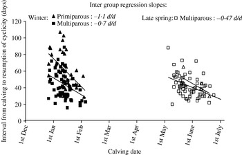
Fig. 4. Effect of the calving date (CALDAY) and parity on the calving to resumption of postpartum cyclicity interval in the Charolais cows at Laqueuille (data reported in this figure are from BE1 data set (3 years×2 calving seasons×parity)).
Numbers in italics report the regression inter-group slopes within calving season and parity.
The biological process by which the calving date acts on the postpartum anoestrus is not clearly established. Two main hypotheses were proposed to explain this relationship. The first is nutritional and assumes that cows calving later in winter have improved pre- and post-calving nutrition (Knight & Nicoll Reference Knight and Nicoll1978). However, insofar as the effect was also observed on well-fed cows (Montgomery et al. Reference Montgomery, Scott and Hudson1985), or on cows with good body condition, this hypothesis was not favoured. The second hypothesis emphasizes the direct influence of daylength on the resumption of the postpartum ovarian activity in cows (Peters & Riley Reference Peters and Riley1982b; Hansen & Hauser Reference Hansen and Hauser1984; King & Macleod Reference King and Macleod1984). This hypothesis is supported by studies that reported a significant negative correlation between the daylength one month before parturition and the acyclic period (Peters & Riley Reference Peters and Riley1982a) or by experimental studies describing an influence of the duration of light on the proportion of cows showing ovarian activity at 70 days postpartum (Garel et al. Reference Garel, Gauthier, Petit and Thimonier1987). Based on these results and on what is known on other species (bison, sheep) about how photoperiod may influence reproduction (Agabriel et al. Reference Agabriel, Bony and Micol1996; Sweeney et al. Reference Sweeney, Donovan, Karsch, Roche and O'Callaghan1997), it was considered that the effect of calving date on PPAI reflects the effect of changes in daylength during the month preceding parturition (Δdaylength=day length 30 days before calving −day length at calving). Considering the latitude of the experimental farm Laqueuille (45·6°N), this variable varies periodically between −89 and +89 min over the year. For each date t, day length has been calculated according to the method proposed by the Institut de Mécanique Céleste et de Calcul des Ephémérides (http://www.bdl.fr/imcce.php?lang=fr.)
Having chosen this working hypothesis, it was tested by comparing the ability of linear statistical models to predict PPAI. Model 1 did not take into account the effect of calving date and only included the effects of parity (multiparous v. primiparous), body condition state at calving (high if BCScalving >2·5 v. low) and bull exposure (early for calving to bull exposure intervals lower than 55 days v. late). The two other models were comparable in all terms except they added a predictive variable to take into account the effect of calving date. Model 2 explicitly included the effect of the calendar date of calving whereas model 3 tested the effect of the variation of daylength during the month preceding calving. These variables were treated as fixed effects. Only the experiment factor was treated as a random effect.
Model 1:
where i is the ith individual in the group, j refers to the experiment and ε is the residual random part of the model.
Model 2: adds calving date covariable and its interaction with season (winter v. spring) or parity
Model 3: adds ΔDaylength covariable and its interaction with parity
The variance–covariance analysis of these models was made using the Proc Mixed procedure (SAS Institute 2000). Models were compared using the Akaike information criteria (AIC=−2ln(ML)+2p), where ML is the maximized likelihood and p is the number of parameters estimated using data; Lancelot et al. Reference Lancelot, Lessnoff and Mcdermott2002). It was considered that the best prediction was associated with the lowest value of the Akaike criteria. This analysis was performed on the whole BE1 data set. Results are reported in Table 2. The lower values of AIC observed for models 2 (AIC=2130) and 3 (AIC=2134) compared to model 1 (AIC=2169) reveal that it is relevant to include the effects of calving date or ΔDaylength to explain and predict the variations in PPAI. Models 2 and 3 account for similar influences of fixed effects (parity, body condition score at calving, bull exposure and the interaction between BCScalving and bull exposure). Such results lead to validation of the hypothesis that considers that the effect of calving date on PPAI can be interpreted as an effect of the photoperiodic variation during the month preceding calving (ΔDaylength).
Table 2. Comparison of three statistical models (ANOVA, proc Mixed) of the postpartum interval (PPAI) (from BE1)

Empty cells in the table correspond to effects that were not tested in the model.
BCS: body condition score (0=emaciated, 5=obese). BCS was considered as a categorical variable because of the low interindividual variability of this variable within BE1 data set.
The response of PPAI to ΔDaylength, adjusted on the data set BE1, is reported in Table 3 according to parity and the interaction between Parity and ΔDaylength. The variation of daylength during the month preceding parturition has a positive effect of 0·4 day per minute for the primiparous cows and a smaller effect (0·09 day/min) for the multiparous cows. Such effects induce a respective maximum variation in PPAI of ±35 days and ±8 days at the year scale. This is consistent with a higher sensitivity of the primiparous cows to the stimuli likely to have an influence on the reproductive function.
Table 3. Influence of the variation in day length (ΔDaylength, min) during the month before calving on the postpartum anoestrous interval (PPAI, days) (from BE1)
The effect of the calving date on PPAI (Calving date_effect) has therefore been formalized with a linear equation of ΔDaylength, whose parameter differs according to parity:
Influence of body condition at calving
The analysis of the BD2 data set (analysis of variance using Proc Mixed, SAS Institute) revealed that below the mean value of 2·5, a variation of BCScalving induces an important variation of PPAI (respectively ±19 v. 28 days per point of BCS for multiparous and primiparous cows). Over the 2·5 threshold, PPAI appeared to be slightly influenced by BCScalving. This observation agrees with the results reported by Lowman (Reference Lowman1985). According to these results, it was considered that the influence of BCScalving on PPAI can be formalized by the following exponential law:
where β and δ are parameters.
Influence of bull exposure
The effect of bull exposure (bull exposure at calving v. no bull exposure) on PPAI was explored by analysing BD3 data set (analysis of variance using Proc Mixed, SAS Institute). Exposing cows to bulls just after parturition significantly shortens the duration of postpartum anoestrus (the decrease is on average −13±3·5 days compared to no bull treatment). Some authors (Stumpf et al. Reference Stumpf, Wolfe, Wolfe, Day, Kittok and Kinder1992; Madrigal et al. Reference Madrigal, Colin and Hallford2001) reported an interaction between body condition at parturition and presence of bulls postpartum on the duration of PPAI: the duration of postpartum anoestrus was shorter in cows of a lower body condition that were in the presence of bulls after calving than in cows with a higher body condition. In order to take into account such an interaction, the effect of bull exposure on PPAI (Bull effect) was formalized using a dependent logistic function of BCScalving:
where Bmax, λ and μ are parameters.
This effect is subtracted from the value of PPAI predicted by the respective effects of CALDAY and BCScalving. Based on the results reported in Table 2, it was considered that females are sensitive to bull exposure when the introduction of the bull occurs quite early after calving, that is to say within the 55 days postpartum period. Because of a lack of available quantitative data relative to the combined effect of bull stimulation and body condition at calving, this expression was calibrated. It was considered that Bmax was equal to 16 days as a compromise between the effects of bull stimulation described by Madrigal et al. (Reference Madrigal, Colin and Hallford2001) and Stumpf et al. (Reference Stumpf, Wolfe, Wolfe, Day, Kittok and Kinder1992) in thin cows. λ and μ were then adjusted to account for a progressive decrease in bull effect from 1·0 to 4·5 BCS at calving (Fig. 5). For BCScalving higher than 3·5, bull effect was considered to be close to zero, assuming that postpartum anoestrous of high fat cows cannot be reduced as they are known to be low already.

Fig. 5. Evolution of bull effect in relation with BCS at calving.
General equation of the PPAI prediction
Finally, prediction of PPAI is made using the following equations including the additive effects of photoperiod, BCS at calving and bull exposure:
If calving to bull exposure interval <55 days:
If calving to bull exposure interval ⩾55 days:
where I and θ are parameters that differ according to parity.
PPAI model calibration (least mean squares method) was made using primiparous cow data from BE1. Calibration on multiparous cow data was not performed as a large part of them could not be considered as independent (repeated measures of same cows). Parameter values are reported in Table 4.
Table 4. Values for fixed and fitted parameters on primiparous Charolais cows (calibration on BE1 primiparous data set)
Oestrous date
After resumption of cyclicity, the oestrous cycles were assumed to succeed one another with a length following a normal distribution with a mean of 21 days and a standard deviation of 1 day (Pleasants Reference Pleasants1997). For simplification, the model considers that all ovulations are associated with an oestrus (Fig. 2) and that the resumption of cyclicity coincides with the first oestrus.
Conception date
The conception date determines the start of gestation. The model considers that all oestrous events are detected by the bull, but that service does not always lead to successful fertilization: the probability of conception varies according to the number of the service and the number of the oestrus that is associated with it. The model does not take into account the possible effects of parity, nutritional state or calving conditions on the probability of conception. However, according to Pleasants & McCall (Reference Pleasants and McCall1993), it was considered that conception rate at the first oestrus after calving is related to PPAI. As there is a suggestion of curvilinearity in this relationship (Pleasants & McCall Reference Pleasants and McCall1993), the relationships between the chance of conception at first oestrus and PPAI were formalized using the following logistic function:
where P 0, P f and Ω are parameters.
The probabilities of conception associated with the various cases of possible services are reported in Table 5. They vary according to the number of the oestrus and the number of the service. These probabilities were estimated from experimental data sets (primiparous cows of BE1 and BE2). They are consistent with those reported by Pleasants et al. (Reference Pleasants, Barton, Morris and Anderson1991) and Pleasants & McCall (Reference Pleasants and McCall1993).
Table 5. Probabilities of conception according to the number of the oestrus and the number of the service
* Values in parentheses were determined from a restricted number of data or were calculated by extrapolation.
Gestation length
GL is the period from conception to parturition, measured in days in the model. It is assumed to follow a normal distribution N(m,σ). Factors that influence gestation length such as breed or birth weight of the calf were not taken into account. Parameters of GL were m=286 and σ=6·5 days.
Calving date
CALDAY differs for each simulated cow in the herd. It is predicted by comparing the value of a random number (RN), generated at the beginning of each simulation between 0 and 100, to the logistic evolution with time of the cumulated proportion of calving cows (CALDAY distribution).
where a and b are parameters and t is time in days.
CALDAY is the time when RN becomes lower than the value of CALDAY distribution.
MODEL BEHAVIOUR AND SENSITIVITY
The model was programmed using ModelMaker® software (Cherwell Scientific Publishing, Oxford).
Behaviour of the system
The behaviour and the sensitivity of the system to initial conditions (calving date, BCScalving, bull exposure and duration of the breeding period) were analysed at the herd level by comparing, for each level of the factor studied, the results obtained from a set of 100 individual cow simulations. When they are not the effects being studied, mean calving date was simulated to be at the beginning of January (varying between the 2nd and the 6th of January according to the simulated calvings data sets that are generated from a stochastic process), BCScalving was considered to be normally distributed with a mean of 2·5 and a standard deviation of 0·5, and bull introduction was fixed at the 25th of February, so that the mean calving to bull exposure interval was around 50 days (varying of ±2 days according to the simulated calvings data sets).
Influence of the calving period
The effects of the calving period on PPAI, first oestrus to conception interval, CI and the conception rate at first oestrus are shown in Fig. 6. Predicted PPAI varied curvilinearly according to the calving period (Fig. 6a). It decreased from October (114±0·2 days) to April (44±0·3 days) and then increased (June: 61±0·6 days). Parallel to the 72 days decrease in PPAI that is predicted by the model from October to April, a 30 day increase in the first oestrus to conception interval (Fig. 6b) was observed. Such a result can be understood considering the relationships between the probability of conceiving at first oestrus (Probaconc1) and PPAI (Table 5), of which one effect is to reduce the conception rate at first oestrus for animals with low PPAI (Fig. 6c). At the CI scale, the effect of calving period remains important and simulations revealed that the objective of a 365 day CI seems to be more realistic for late winter calvings than for autumn calvings (CI=400±0·5 days in October v. 362±1·2 days in April, Fig. 6d).

Fig. 6. Influence of the calving period on the predicted PPAI (a), first oestrous to conception interval (b), conception rate at first oestrus (c) and calving interval (d) (means±s.e., n=100 individual cow simulations per level of simulated calving period).
Influence of body condition at calving
The effects of three mean levels of body condition at calving (1·5, 2·5 and 3·5) were studied on PPAI. As expected, the model predicted a higher BCScalving effect in very thin cows (8·5±0·57 days for BCScalving=1·5) than in fatter ones (1·6±0·10 days for BCScalving=2·5 and 0·2±0·02 days for BCScalving=3·5). However for a mean calving to bull exposure interval equal to 50±0·9 days, it was observed that the bull effect, which depends on BCScalving and plays in an opposite way, may cancel the influence of BCScalving (Bull_effect=−8·5±0·42 days for BCScalving=1·5, −5·2±0·31 days for BCScalving=2·5 and −1·12±0·12 days for BCScalving=3·5), so that predicted PPAI did not really differ according to BCS at calving (84±1·2 days for BCScalving=1·5, 81±0·9 days for BCScalving=2·5 and 84±0·7 days for BCScalving=3·5). At the scale of the whole reproductive cycle (CI), there was no effect of BCScalving on predicted CI (385±1·1 days for BCScalving=1·5, 383±0·9 days for BCScalving=2·5 and 383±0·9 days for BCScalving=3·5).
Influence of body condition at calving and bull exposure
The combined influences of BCS at calving and bull exposure on the reproductive performance were studied considering three levels of BCScalving (1·5, 2·5 and 3·5) and three levels of bull exposure (bull introduction at 50, 80 and 110 days after the beginning of calvings). For all of these combined levels a set of 100 individual cow simulations was performed. The mean calving date varied between 2 January and 6 January according to the simulated data set. Mean calving to bull exposure intervals were 26±0·8, 54±0·8 and 86±0·8 days for the 50, 80 and 110 bull treatments, respectively.
As expected, when bull exposure occurred early after calving (treatment 50), the model accounted for a more important bull effect for thin (BCScalving=1·5) than for fat cows (BCScalving=3·5): −14·7±0·1 days v. −1·6±0·1 days (Fig. 7). The parameter values used for these simulations induced a greater effect of bull exposure than of BCS calving on PPAI. Consequently, the model simulated lower average PPAI in thin cows exposed early to a bull (79±0·7 days) than in fat cows (86±0·7 days): when thin cows were exposed early to a bull, the bull effect on PPAI (–14·7 days) was about twice as high as the positive BCScalving_effect (+8 days) and thus contributed to a severe decrease in the predicted PPAI value, unlike what was observed in fat cows (Fig. 7).

Fig. 7. Changes in BCScalving effect and bull effect according to BCS at parturition and to bull treatment (means±s.e., n=100 individual cow simulations).
Bull treatments 50, 80 and 110, respectively, refer to periods (in days) from the first calving within the herd to the day of bull introduction.
For bull treatment 80, which corresponds to mean calving to bull exposure intervals (54±0·8 days) close to those observed in our farm conditions, no obvious differences in PPAI were observed between the three BCScalving levels tested (86±1·2 days for BCScalving=1·5, 82±0·9 days for BCScalving=2·5 and 84±0·7 days for BCScalving=3·5). Such results are in contradiction to the effect of body condition that is generally reported in the literature. They can be attributed to the choice of β and Bmax values that were fixed by expertise and determine the respective amplitudes of BCScalving and bull effects. The influence of Bmax parameter values on the predicted PPAI will be discussed further.
Influence of the length of the mating period
The sensitivity of reproductive efficiency to the duration of the mating period (30, 60, 90 or 120 days) was tested on a group of 100 primiparous cows calving in winter (mean calving date: 5 January). The mean interval from parturition to bull exposure was 50±0·9 days. As expected, the mean simulated PPAI did not differ according to the treatments and were of 81±0·9 days. Decreasing the duration of the mating period induced an increase in the percentage of non-pregnant cows (Table 6). A 30-day breeding period significantly affected the reproductive efficiency of the herd as only 48% of cows succeeded in conceiving within this period. Mean calving to conception intervals and CIs of pregnant cows were 10 days shorter for treatment 30 compared to treatment 120 (Table 6).
Table 6. Effects of the duration of the breeding period on components of the reproductive efficiency (values are means±standard errors of 100 individual simulationsFootnote *)
* Initial values of the simulations: mean calving date: 5 January, mean BCScalving: 2·5, mean calving to bull exposure interval: 50 days.
Calving distribution
As the model simulates the CI of each cow, it is possible to study the evolution of calving distributions (evolution with time of the proportion of cows that have calved) between two successive years. The initial conditions considered for this simulation were the same as those fixed for the treatment 120 described in the previous paragraph. The model predicted that the mean calving date of the second calving cows (year 2: 27 January) occurred 21 days later than the mean calving date observed the preceding year (year 1: 6 January) (Fig. 8). Calving distribution was also spread over a longer period in year 2 (116 days) than in year 1 (101 days). Such a result illustrates that culling and replacement decisions linked to the analysis of predicted CI are a way to keep the average calving date in a herd constant.

Fig. 8. Evolution of the calving distribution between two successive years. Distributions were determined from n=100 simulated primiparous cows with a mean calving date being the 6th of January, a mean BCScalving of 2·5, and a mean calving to bull interval of 50 days.
Sensitivity to parameter values
The sensitivity of the model to a ±10% variation of θ (ΔDaylength effect), Ω (probability of conception at first oestrus according to PPAI), μ and Bmax (bull effect) parameters was tested. The indicator of sensitivity is S_V (V p+10−V p−10)/V pref), where V p+10 is the simulated value of the variable V for a parameter value set to p=p ref+10%×p ref (Thornley & France Reference Thornley and France2007).
The evolution of S_PPAI to a variation of θ is reported in Fig. 9. Of course, a 10% variation in θ value induced a change in the ΔDaylength effect (θ×ΔDaylength) of a similar amplitude (Fig. 9a). However, it appeared that S_PPAI evolved according to the calving date with a higher sensitivity at the beginning of April, when ΔDaylength was highly negative (Fig. 9b).

Fig. 9. Sensitivity of the photoperiodic effect (a) and of PPAI (b) to a±10% change in the value of θ parameter (I=84·6, BCScalving=2·5 and Bull_effect=0).
The sensitivity of the system to changes in Ω parameter value is reported in Table 7. For a given PPAI, the probability of conception at the first oestrus increased with the value of Ω parameter. For winter calvings (occurring around 5 January), a ±10% variation in the Ω parameter value induced important changes in the first oestrus to conception interval (respectively +15 and −22%, Table 7). This response is very much reduced for spring calvings (occurring around the 4th of April) (+2·8 and −3·6%, Table 7). So, the sensitivity of the system to a change in Ω parameter value depends on the predicted length of PPAI: it is greater for high than for low PPAI. At the scale of the CI, a ±10% variation in Ω parameter value had negligible effects (Table 7).
Table 7. Influence of a ±10% change in Ω parameter on the reproductive components of calving interval. Values are expressed as means±standard errors (n=100 simulations per Ω value tested. Two mean calving dates were considered: 5 January and 4 April. Bull entry occurred 76 days after the beginning of calvings and the breeding period lasted 144 days. Mean BCS at calving was 2·5)

Values in italics report the variation of the variables (%) induced by the change in the parameter value.
A ±10% change in μ parameter value induced an important variation in bull_effect. (−26% for μ−10% and +18% for μ+10%). However, the associated relative changes in PPAI were quite restricted (+1·7% for μ−10% and −1·2% for μ+10%). Thus, the reproductive performance of the cow seems not very sensitive to a change in μ parameter.
The sensitivity of the system to the amplitude of the bull effect (Bmax parameter) was undertaken to study the response of PPAI to the combined effects of BCScalving and bull exposure. The changes of Bull_effect and PPAI were analysed for different values of Bmax (Bmax−80%=3·2, Bmax−60%=6·4, Bmax−40%=9·6, Bmax−20%=12·8, Bmax−10%=14·4, Bmaxref=16 and Bmax+10%=17·6) and three levels of body condition at calving (BCScalving=1·5, 2·5 and 3·5). Main results are reported in Figs 10 and 11. Whatever the BCScalving, the bull effect increased proportionally with Bmax. However, this variation differed according to the body condition of cows: it was very low for fat cows (from −0·2 to −1·2 days for Bmax varying from 3·2 to 17·6), intermediate for 2·5 BCScalving cows (from −1·0 to −5·0 days) and the highest for thin cows (from −1·5 to −9·0 days) (Fig. 10). For Bmax values lower than 14·4, predicted PPAI was always higher in thin cows (Fig. 11), which is in agreement with the literature. For Bmax values up to 14·4, there tended to be no difference in PPAI between thin and fat cows. For these Bmax values, it appeared that the result of the cumulative effects of BCS at calving and bull exposure was similar for thin and fat cows (between 0 and −1 day, Fig. 10). Such unexpected behaviour was also observed for cows with an intermediate body condition score at calving (2·5): from the Bmax threshold value of 6·4, PPAI of these cows appeared to be lower than PPAI of fat cows (Fig. 11). This result can be partly imputed to the logistic equation describing the variation of bull effect according to BCS at calving (Fig. 5, Bmax=16) that predicts a mean bull effect of −8·3 days for 2·5 BCS cows and of only −0·9 day for 3·5 BCS cows. From a Bmax value up to 6·4, it appears that the cumulative effects of BCS at calving and bull exposure on PPAI become more negative for 2·5 BCS cows than for 3·5 BCS cows (Fig. 10). The choice of the parameter values fixed for BCScalving effect and for bull effect (Table 4) would have to be re-evaluated for further uses of the model. For a practical use of the model a Bmax value lower or equal to 6·4 days should be recommended as it accounts for behaviour in agreement with observations reported in the literature: higher PPAI in thin cows but not much difference in PPAI of 2·5 and 3·5 BCS cows (Fig. 11).

Fig. 10. Effects of changes in Bmax parameter values on BCScalving effect (![]() , BCScalving=1·5;
, BCScalving=1·5;![]() , BCScalving=2·5;
, BCScalving=2·5;![]() , BCScalving=3·5), Bull effect (
, BCScalving=3·5), Bull effect (![]() , BCScalving=1·5;
, BCScalving=1·5;![]() , BCScalving=2·5;
, BCScalving=2·5;![]() , BCScalving=3·5) and their sum (
, BCScalving=3·5) and their sum (![]() , BCScalving=1·5;
, BCScalving=1·5; ![]() , BCScalving=2·5;
, BCScalving=2·5; ![]() , BCScalving=3·5). (n=100 individual cow simulations per combined level of bull and BCScalving. Mean calving date is 5th of January. Bull entry occurs on the 25th of February, 76 days after the beginning of calvings. Mean calving to bull exposure interval was 51±0·8 days.)
, BCScalving=3·5). (n=100 individual cow simulations per combined level of bull and BCScalving. Mean calving date is 5th of January. Bull entry occurs on the 25th of February, 76 days after the beginning of calvings. Mean calving to bull exposure interval was 51±0·8 days.)
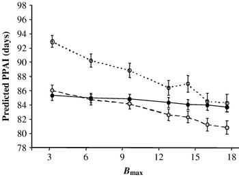
Fig. 11. Effects of changes in Bmax parameter values on the postpartum anoestrous interval (PPAI) (○, BCScalving=1·5;![]() , BCScalving=2·5; ●, BCScalving=3·5). (n=100 individual cow simulations per combined level of bull and BCScalving. Mean calving date is the 5th of January. Bull entry occurs the 25th of February, 76 days after the beginning of calvings. Mean calving to bull exposure interval was 51±0·8 days.)
, BCScalving=2·5; ●, BCScalving=3·5). (n=100 individual cow simulations per combined level of bull and BCScalving. Mean calving date is the 5th of January. Bull entry occurs the 25th of February, 76 days after the beginning of calvings. Mean calving to bull exposure interval was 51±0·8 days.)
MODEL EVALUATION: ABILITY TO PREDICT PPAI
Evaluation of the model was only performed on the PPAI component of reproductive performance as it is the main original part of the model compared to previous published work. The predictive quality of the model was tested by comparing predicted to observed PPAI of primiparous cows. This evaluation was not performed on multiparous cow data because many of them were not independent (repeated measures on the same cows). Parameter values of the PPAI model were estimated from the primiparous winter calving cows from BE1 dataset (n=109), whereas BE2 (n=188) was used to perform the external validation of the model.
Only the value of the I parameter (intercept of the model), which depends on the data set in relation with the frequency of progesterone measurements, was re-estimated for the external validation. The quality of the prediction was assessed on the basis of criteria proposed by Gauch et al. (Reference Gauch, Gene Hwang and Fick2003) which account for the deviation between model-based and measured values, X n and Y n. The mean square deviation (MSD) between X and Y (MSD=Σ(X n−Y n)2/N, where N is the number of observations) is the main statistic for this purpose, as it equates to deviations around the 1:1 line of equality whereas the mean square error often reported for regressions uses deviations around the regression line (Gauch et al. Reference Gauch, Gene Hwang and Fick2003). The partitioning of MSD has three components. The first component is the squared bias (![]() , where
, where ![]() and
and ![]() are the respective means of X n and Y n), which arises from these two means being unequal. The second component is the mean square for the nonunity slope ((NU=(1−b)2×(Σx n2/N), where b is the slope of the least square regression of Y on X, and
are the respective means of X n and Y n), which arises from these two means being unequal. The second component is the mean square for the nonunity slope ((NU=(1−b)2×(Σx n2/N), where b is the slope of the least square regression of Y on X, and ![]() is the deviation from the mean). The third component is the mean square of LC (LC=(1−R 2)×(Σy n2/N), where R 2 is the square of the correlation and
is the deviation from the mean). The third component is the mean square of LC (LC=(1−R 2)×(Σy n2/N), where R 2 is the square of the correlation and ![]() is the deviation from the mean).
is the deviation from the mean).
For this internal validation, the mean predicted PPAI does not differ from the observed PPAI (81·8±1·3 days v. 81·4±2·3 days). Root MSD reaches 17 days and the model accounts for 47% of the observed dispersion. The lack of correlation (LC) represents the major component of MSD (97%), whereas translation (SB) and rotational bias (NU) have a very low contribution to MSD (0 and 3%, respectively).
This model was then evaluated by comparing model-based predictions to an independent data set (Primiparous cows from BE2 data set). Results are reported in Fig. 12. They are similar to the results obtained with the internal evaluation. The model only accounts for 39% of the variability (root MSD=18 days, similar to the root MSD observed for internal validation). However, as NU and SB are very low (Fig. 12), we considered that the structure of the PPAI model can be validated.

Fig. 12. Comparison of observed to predicted values of post-partum interval (primiparous cows of BE2 data set, n=188, external evaluation). The vertical bar represents the decomposition of MSD; ■, lack of correlation; □, squared bias;![]() , non-unity slope.
, non-unity slope.
DISCUSSION AND CONCLUSION
The model of beef cow reproductive performance presented here makes it possible to study the direct and induced effects of factors likely to be controlled by the livestock farmer (body condition of the cows at calving, bull entry and exit dates, calving period) on the various components of the female reproductive performance (postpartum anoestrus, calving-conception interval, calving–calving interval and pregnancy rate).
This model focuses on the individual cow but can also be used to obtain an estimation of response mean and variance for reproductive traits at the herd level. Two main sources of variability are considered: one is generated by the stochastic nature of some of the components of the reproductive process (oestrous cycle length, probability of conception at first oestrus, gestation length). The second comes from variations in the ‘cause–effect’ responses that are induced by differences in the biological characteristics of the individuals (parity, body fatness at calving, calving date). This model illustrates an intermediate position between the entirely deterministic approach proposed by Denham et al. (Reference Denham, Larsen, Boucher and Adams1991), and the stochastic approach developed by Pleasants (Reference Pleasants1997) or Azzam et al. (Reference Azzam, Kinder and Nielsen1990).
In the current study, most of the effort was directed at conceptualizing and formalizing the effects of the major variables known to influence the resumption of cyclicity after parturition. A bibliographical work enabled a prioritization of the importance of the factors involved in this resumption and select those likely to be influenced by management decisions. The intensity of suckling, known to have a major effect on postpartum anoestrus in beef cows (Williams Reference Williams1990), has therefore not been taken into account in the model insofar as the farming systems studied do not practise restricted suckling. The effect of the postpartum level of feeding was not chosen either, in spite of the importance that certain authors attribute to it (Sanz et al. Reference Sanz, Bernues, Villalba, Casasus and Revilla2004).
On the other hand, particular attention was paid to the influence of the calving date on the resumption of postpartum ovarian activity. Unlike the modelling approach proposed by Pleasants (Reference Pleasants1997), it was not considered that the length of anoestrus is a normally distributed random variable depending on the calving date of the cow. A biological interpretation of this effect is suggested, emphasizing that the influence of the calving date accounts for a sensitivity of the ovarian function to the variation of the photoperiod during the month before calving. Such a biological interpretation of calving date is consistent with previous studies that tend to demonstrate that, even if ovulatory activity is not seasonal in cows, photoperiodic rhythm is still present and may induce a seasonal pattern of biological functions. Such an influence was observed for milk production and quality (Coulon et al. Reference Coulon, Chilliard and Remond1991) and is strongly implicated in postpartum ovulatory activity (Hauser Reference Hauser1984; Chemineau et al. Reference Chemineau, Malpaux, Brillard and Fostier2007).
The integration of the daylength effect in the model of PPAI improves the quality of the prediction compared to a model only integrating the effects of parity, body condition at calving and bull exposure. In particular it qualifies and formalizes the season effect often quoted in the literature (Short et al. Reference Short, Bellows, Staigmiller, Berardinelli and Custer1990; Sanz et al. Reference Sanz, Bernues, Villalba, Casasus and Revilla2004). The effect of calving period on PPAI predicts an average reduction of −0·3 day per additional day of calving between October and June. This result is in agreement with the values reported by Peters & Riley (Reference Peters and Riley1982a) and Pleasants (Reference Pleasants1997) for autumn to winter calvings. However, the main originality of the current approach lies in the fact that such a result is obtained by considering a direct effect of the photoperiod associated with the calving period and not a direct stochastic effect of the calving date as proposed by Pleasant (Reference Pleasants1997).
The external evaluation of the PPAI model shows that a large part of the total variance (about 50%) is not explained by the deterministic considered effects. Such a result leads to minimizing the ability of the model to predict accurately the time of the postpartum resumption of ovarian cyclicity of a given cow. However, the evaluation of the PPAI model showed that its structure can be validated because of very little bias of translation and rotation. In order to improve the predictive quality of the model, modifications can be proposed as taking more account of the influence of nutrition. Beyond the body condition at calving, always indicated as a factor of importance (Short et al. Reference Short, Bellows, Staigmiller, Berardinelli and Custer1990; Ducrot et al. Reference Ducrot, Grohn, Humblot, Bugnard, Sulpice and Gilbert1994), the energy level after calving can also significantly influence PPAI, particularly in primiparous cows for which all known nutritional effects are emphasized (Agabriel et al. Reference Agabriel, Grenet and Petit1992; Sanz et al. Reference Sanz, Bernues, Villalba, Casasus and Revilla2004). The framework proposed by Friggens (Reference Friggens2003) to formalize the effects of body fatness at calving and lipid mobilization after parturition on the reproductive priorities of the female (lactation v. reproduction) should be considered to improve the model. Another factor that should to be taken into account to improve the accuracy of the PPAI model is the influence of calving difficulties that are usually recorded in a herd and contribute to variation in the postpartum anoestrous (Ducrot et al. Reference Ducrot, Grohn, Humblot, Bugnard, Sulpice and Gilbert1994; Humblot et al. Reference Humblot, Grimard, Ribon, Khireddine, Dervishi and Thibier1996).
The analysis of the behaviour of the model in relation to the combined effects of body condition and bull exposure highlighted the need for a better appreciation of their respective amplitude and interaction. Indeed, these two effects are opposed in the model, since the first increases the value of PPAI predicted by the effect of the photoperiod, whilst the second decreases it. The bull effect was modelled as a function of the body condition at calving in order to account for the interaction between these two effects highlighted in the literature. The parameter values chosen in the simulations to quantify the bull effect were estimated from literature and adapted by expertise. This set of parameter values induced an unexpected response, as fat cows tended to have similar postpartum anoestrus to thin cows, which is in contradiction with the literature (Petit et al. Reference Petit, Jarrige, Russel, Wright, Jarrige and Béranger1992; Wright et al. Reference Wright, Rhind, Whyte and Smith1992). Such a result does not call into question the structure of the model but suggests collecting more data to better evaluate the respective effects of the body condition and its interaction with bull exposure, therefore more work is necessary to confirm this. In the present experimental data sets, the variability of the cows' body condition was undoubtedly too low. Given the very limited number of studies relating to these two combined effects, it would be necessary to develop additional experiments in this field.
The validation work undertaken by comparing model-based to measured values of PPAI is original, as it appears that no previous model of reproductive performance of cows has been evaluated on the basis of individual data (Blanc et al. Reference Blanc, Martin and Bocquier2001).
The model makes it possible to better understand the incidence of management choices relative to herd nutrition and reproduction (period and duration) on the reproductive performance of the herd. Its partially deterministic structure makes it possible to consider the development of a tool that may improve heat detection in beef herds using artificial insemination. By predicting the distribution of oestrous times, it thus could help determining target periods for focusing oestrous observations according to the average body condition and calving date of the cows.
Special thanks go to the staff of Laqueuille and Le Pin experimental farms for data collection. Thanks are also due to Jane Curtis for improving the English.


