3.1. The Basilisk solver

We solve the three-dimensional, incompressible, two-phase Navier–Stokes equations using the open-source solver Basilisk (Popinet Reference Popinet2009, Reference Popinet2015; van Hooft et al. Reference van Hooft, Popinet, van Heerwaarden, van der Linden, de Roode and van de Wiel2018):

(3.1)\begin{gather} \partial_t\boldsymbol{u}+\boldsymbol{\nabla}\boldsymbol{\cdot}(\boldsymbol{u}\boldsymbol{u}) = \frac{1}{\rho}\left[-\boldsymbol{\nabla} p + \boldsymbol{\nabla}\boldsymbol{\cdot} (\mu(\boldsymbol{\nabla} \boldsymbol{u}+\boldsymbol{\nabla} \boldsymbol{u}^{T}))\right] + \frac{\gamma}{\rho}\kappa\delta_s\boldsymbol{n}, \end{gather}

(3.2)\begin{gather}\boldsymbol{\nabla}\boldsymbol{\cdot}\boldsymbol{u} = 0, \end{gather}

(3.3)\begin{gather}\frac{\partial \mathcal{T}}{\partial t} + \boldsymbol{u} \boldsymbol{\cdot} \boldsymbol{\nabla}\mathcal{T} = 0, \end{gather}

where $\boldsymbol {u}$, $p$, $\gamma$, $\mu$, $\rho$, $\kappa$, $n$ and $\mathcal {T}$ are the velocity, pressure, surface tension coefficient, viscosity, density, curvature, interface normal and volume fraction fields, respectively. The solver has been extensively validated for complex interfacial flows (Popinet Reference Popinet2015; Farsoiya, Mayya & Dasgupta Reference Farsoiya, Mayya and Dasgupta2017; Ruth et al. Reference Ruth, Mostert, Perrard and Deike2019; Gumulya et al. Reference Gumulya, Utikar, Pareek, Evans and Joshi2020; Berny et al. Reference Berny, Deike, Séon and Popinet2020; Mostert & Deike Reference Mostert and Deike2020). It uses the projection method to compute the velocity and pressure and the geometric volume-of-fluid method for the evolution of the interface between two immiscible fluids (Tryggvason, Scardovelli & Zaleski Reference Tryggvason, Scardovelli and Zaleski2011). The Piecewise Linear Interface Calculation geometric interface and flux reconstruction ensures a sharp representation of the interface (Scardovelli & Zaleski Reference Scardovelli and Zaleski1999; Marić, Kothe & Bothe Reference Marić, Kothe and Bothe2020) and is combined with an accurate height-function curvature calculation and a well-balanced, continuum surface tension model (Brackbill, Kothe & Zemach Reference Brackbill, Kothe and Zemach1992; Popinet Reference Popinet2018).

3.2. One-fluid formulation for mass transfer of dilute gas

The continuous formulation for mass transfer that we use in this study has been independently developed by Haroun et al. (Reference Haroun, Legendre and Raynal2010) and Marschall et al. (Reference Marschall, Hinterberger, Schüler, Habla and Hinrichsen2012). We have implemented the concentration diffusion of dilute gas (Haroun et al. Reference Haroun, Legendre and Raynal2010) using the harmonic mean diffusion coefficient as verified by Deising et al. (Reference Deising, Marschall and Bothe2016). Note that the present study investigates the mass transfer of dilute gas present in the bubble where the effects of loss of volume and phase change are ignored. Numerical methods for phase change require changes in the volume-of-fluid advection equation and continuity equation (Tanguy et al. Reference Tanguy, Sagan, Lalanne, Couderc and Colin2014; Fleckenstein & Bothe Reference Fleckenstein and Bothe2015; Maes & Soulaine Reference Maes and Soulaine2020; Scapin et al. Reference Scapin, Costa and Brandt2020). The time evolution of the $j$th gas concentration $c_{l/g,j}$ for the liquid phase $l$ or the gas phase $g$ is given by (Standart Reference Standart1964; Haroun et al. Reference Haroun, Legendre and Raynal2010)

(3.4)\begin{equation} \frac{\partial c_{l/g,j}}{\partial t} + \boldsymbol{\nabla}\boldsymbol{\cdot} (\boldsymbol{u} c_{l/g,j})={-}\boldsymbol{\nabla} \boldsymbol{\cdot} (J_{l/g,j}). \end{equation}

The continuity of normal fluxes across the interface $\varSigma$ (Standart Reference Standart1964; Bothe & Fleckenstein Reference Bothe and Fleckenstein2013) is

(3.5)\begin{equation} [\kern-1pt[ (c_j(\boldsymbol{u} -\boldsymbol{ u}_\varSigma) + \boldsymbol{J}_{j} )\boldsymbol{\cdot} \boldsymbol{n}_\varSigma ]\kern-1pt] = 0, \end{equation}

where $\boldsymbol {u}_\varSigma$ is the interface velocity. As we assume that the transfer of a dilute component does not cause volume change, (3.5) reduces to

(3.6)\begin{equation} \boldsymbol{J}_{l,j} \boldsymbol{\cdot} \boldsymbol{n}_\varSigma = \boldsymbol{J}_{g,j} \boldsymbol{\cdot} \boldsymbol{n}_\varSigma. \end{equation}

The standard assumption of continuous chemical potentials which is good for most applications at interface $\varSigma$ results in Henry's law (we refer interested readers to Bothe & Fleckenstein (Reference Bothe and Fleckenstein2013) for a discussion on local chemical equilibrium and the generalized Henry's law):

(3.7)\begin{equation} c_{l,j} = c_{g,j} \alpha_j, \end{equation}

where the dimensionless ratio of the liquid-phase concentration to the gas-phase concentration of the component transferred $\alpha _j$ is called the Henry's law solubility constant (Sander Reference Sander2015) (solubility hereafter). The problem investigated is isothermal and there is no bubble breakup or large deformation of the interface which can change the pressure inside the bubble significantly. Hence, solubility which at least depends on temperature and pressure (Bothe & Fleckenstein Reference Bothe and Fleckenstein2013) is assumed to be constant. Introducing variables for the one-fluid formulation which is valid for both phases $l$ and $g$ and for gas $j$, we get

(3.8a,b)\begin{equation} c_j = \mathcal{T} c_l + (1-\mathcal{T})c_g,\quad J_j = \mathcal{T} J_l + (1-\mathcal{T})J_g, \end{equation}

and the flux is given by

(3.9)\begin{equation} J_j ={-} (\mathcal{T} \mathscr{D}_{jl} \boldsymbol{\nabla} c_l + (1-\mathcal{T}) \mathscr{D}_{jg} \boldsymbol{\nabla} c_g). \end{equation}

The diffusivity for the interfacial cells is calculated using the harmonic mean of the two diffusivities of the gas inside and outside the bubble (Haroun et al. Reference Haroun, Legendre and Raynal2010),

(3.10)\begin{equation} \mathscr{D}_{j} = \frac{\mathscr{D}_{jg} \mathscr{D}_{jl}}{\mathscr{D}_{jl}(1-\mathcal{T})+\mathscr{D}_{jg}\mathcal{T}}, \end{equation}

to get a single equation for both phases:

(3.11)\begin{equation} \frac{\partial c_j}{\partial t} + \boldsymbol{\nabla}\boldsymbol{\cdot} (\boldsymbol{u} c_j)=\boldsymbol{\nabla} \boldsymbol{\cdot} \left( \mathscr{D}_j\boldsymbol{\nabla} c_j - \mathscr{D}_j\left(\frac{c_j(\alpha_j-1)}{\alpha_j \mathcal{T}+(1-\mathcal{T})}\right) \boldsymbol{\nabla} \mathcal{T}\right). \end{equation}

The coefficient of $c_j$ in the second term on the right-hand side of (3.11) can be written as $\beta _j$:

(3.12)\begin{equation} \frac{\partial c_j}{\partial t} =\boldsymbol{\nabla} \boldsymbol{\cdot} \left( \mathscr{D}_j\boldsymbol{\nabla} c_j + \beta_j c_j \right). \end{equation}

Using a time-implicit Euler discretization,

(3.13)\begin{equation} \frac{ c^{n+1}_j-c_j^{n}}{\Delta t} =\boldsymbol{\nabla} \boldsymbol{\cdot} \left( \mathscr{D}_j\boldsymbol{\nabla} c^{n+1}_j + \beta_j c^{n+1}_j \right), \end{equation}

and rearranging the implicit terms gives

(3.14)\begin{equation} \boldsymbol{\nabla} \boldsymbol{\cdot} \left( \mathscr{D}_j\boldsymbol{\nabla} c^{n+1}_j + \beta_j c^{n+1}_j \right) -\frac{c_j^{n+1}}{\Delta t}={-}\frac{c_j^{n}}{\Delta t}. \end{equation}

Equation (3.14) is a set of linear equations which is solved efficiently using the multigrid method (Popinet Reference Popinet2015).

The solubility boundary condition (3.7) presents a discontinuity for the concentration field across the interface similar to the volume fraction field $\mathcal {T}$. As discussed by Bothe & Fleckenstein (Reference Bothe and Fleckenstein2013), a non-consistent advection leads to artificial diffusion for concentration. For a consistent advection two tracer fields $\phi _{g}$ and $\phi _{l}$ associated with the volume of fluid $\mathcal {T}$ are defined:

(3.15a,b)\begin{equation} \phi_l = c_l \mathcal{T},\quad \phi_g= c_g(1-\mathcal{T}). \end{equation}

Using (3.7) and (3.8a,b), we get

(3.16a,b)\begin{equation} \phi_{l,j} = \frac{c^{n+1}_j\,\alpha_j\,\mathcal{T}}{\alpha_j \mathcal{T}+(1-\mathcal{T})}, \quad \phi_{g,j} = \frac{c^{n+1}_i(1-\mathcal{T})}{\alpha_j \mathcal{T}+(1-\mathcal{T})}. \end{equation}

The advection equation for $\phi _{g/l}$ reads

(3.17)\begin{equation} \frac{\partial \phi_{g/l}}{\partial t} + \boldsymbol{\nabla}\boldsymbol{\cdot} (\boldsymbol{u} \phi_{g/l})=0 \end{equation}

and is solved using the volume-of-fluid associated fields (López-Herrera et al. Reference López-Herrera, Ganan-Calvo, Popinet and Herrada2015) which guarantees strictly non-diffusive transport close to the interface. The concentration tracer is updated after advection using

(3.18)\begin{equation} c_j = \phi_{g,j} + \phi_{l,j}. \end{equation}

3.3. Validation

We validate the numerical methods and their implementation for static and rising bubble cases.

3.3.1. Diffusion from a static bubble

We propose a new test case of diffusion from a constant-size, static, spherical bubble. Test cases are available for concentration profiles in the case of a planar interface in Bird, Stewart & Lightfoot (Reference Bird, Stewart and Lightfoot2002) and Haroun et al. (Reference Haroun, Legendre and Raynal2010). We provide the solution for the transient concentration both inside and outside the spherical bubble in the form of integrals which are then evaluated numerically.

Consider a static axisymmetric bubble of radius $R_0=d_0/2$. The diffusivities of the gas are $D_g$ and $D_l$ for the gas and liquid phase, respectively. The one-dimensional transient concentration diffusion for a spherical geometry for both inside and outside the bubble is given by

(3.19a,b)\begin{equation} \frac{\partial c_g}{\partial t} = \mathscr{D}_g \frac{1}{r^{2}}\frac{\partial }{\partial r}\left(r^{2}\frac{\partial c_g}{\partial r}\right), \quad \frac{\partial c_l}{\partial t} = \mathscr{D}_l \frac{1}{r^{2}}\frac{\partial }{\partial r}\left(r^{2}\frac{\partial c_l}{\partial r}\right). \end{equation}

Applying the Laplace transform to the above equations, we get $\tilde {c}(s)=\mathcal {L}[c(t)]$,

(3.20a,b)\begin{equation} \frac{\textrm{d}^{2}\tilde{c}_g}{\textrm{d}r^{2}} +\frac{2}{r}\frac{\textrm{d}\tilde{c}_g}{\textrm{d}r}-\frac{s}{\mathscr{D}_g}\tilde{c}_g+\frac{1}{\mathscr{D}}c_{g0} = 0, \quad \frac{\textrm{d}^{2}\tilde{c}_l}{\textrm{d}r^{2}} +\frac{2}{r}\frac{\textrm{d}\tilde{c}_l}{\textrm{d}r}-\frac{s}{\mathscr{D}_l}\tilde{c}_l + \frac{1}{\mathscr{D}}c_{l0} = 0. \end{equation}

Given boundary conditions $r\tilde {c}_g\rightarrow 0$ as $r\rightarrow 0$, $\tilde {c}_l\rightarrow 0$ as $r\rightarrow \infty$, $[\kern-1pt[ \mathscr {D} \partial \tilde {c}/\partial r ]\kern-1pt] = 0$ and $\tilde {c}_l/\tilde {c}_g=\alpha$ at $r=R_0$, the concentrations (Laplace transformed) inside the bubble $\tilde {c}_g$ and outside $\tilde {c}_l$ are given by

(3.21a,b)\begin{equation} \tilde{c}_g(s,r) = \frac{c_{g0}}{s}\left( 1 - \frac{2 }{ \zeta(s) r}\sinh\left[\lambda_g(s) r\right]\right), \quad \tilde{c}_l(s,r) = \frac{ \xi c_{g0}}{s \zeta(s) r}\exp{\left[-\lambda_l(s) r\right]}, \end{equation}

where

(3.22)\begin{equation} \left.\begin{gathered} \lambda_{g/l} = \sqrt{\frac{s}{\mathscr{D}_{g/l}}}, \quad \zeta(s) = \frac{\xi \exp\left[-\lambda_l R_0\right]}{\alpha\,R_0} + \frac{2}{R_0}\sinh(\lambda_g R_0), \\ \xi(s) = \frac{2 \mathscr{D}_g(\lambda_g R_0 \cosh(\lambda_g R_0)-\sinh(\lambda_g R_0))}{\mathscr{D}_l \exp[-\lambda_l R_0](1 + \lambda_l R_0)}, \quad c_{g0}=c_g(0,r),\quad c_{l0} = 0. \end{gathered}\right\} \end{equation}

Equation (3.21a,b) can be inverted using the Cauchy residue theorem (using keyhole contour as discussed in Farsoiya, Roy & Dasgupta (Reference Farsoiya, Roy and Dasgupta2020)):

(3.23)\begin{gather} c_g(t,r) ={-}\frac{2 c_{g0}}{{\rm \pi} r}\int_{0}^{\infty}\frac{1}{x}\mathrm{Im}\left\{ \frac{\sinh(\lambda_g({-}x) r)}{\zeta({-}x)}\right\}\exp[{-}xt]\,{\textrm{d} x}, \end{gather}

(3.24)\begin{gather}c_l(t,r) = \frac{c_{g0}}{{\rm \pi} r}\int_{0}^{\infty}\frac{1}{x}\mathrm{Im}\left\{ \frac{\xi({-}x)}{\zeta({-}x)}\exp{\left[-\lambda_l({-}x) r\right]}\right\}\exp[{-}xt] \, {\textrm{d} x}, \end{gather}

where $\mathrm {Im}(\cdot )$ is the imaginary part of a complex number. We validate the results of the Basilisk solver against (3.23) and (3.24) (using the numerical integration functions based on double-exponential quadrature in Wolfram Research, Inc. (2020)) in figure 1.

Figure 1. Diffusion from a static bubble, comparing the numerical results with (3.23) and (3.24). (a) Concentration inside the bubble at $r/d_0=0.25$. (b) Concentration outside the bubble at $r/d_0=0.75$. (c) Radial profile at time $t\mathscr {D}_l/d_0^{2}=1.2$. (d) Maximum relative error at different resolutions $\max |c_{11}-c_n|/c_{11}$, where $c_{11}$ and $c_n$ are numerical solutions at resolution $2^{11}$ and lower, respectively, and for different solubilities $\alpha$, displaying first-order convergence. The scripts sufficient to reproduce these results are provided in Farsoiya, Popinet & Deike (Reference Farsoiya, Popinet and Deike2020a).

A static bubble of diameter $d_0/L=0.2$, diffusivity ratio $\mathscr {D}_g/\mathscr {D}_l=10$ and solubility $\alpha =10^{-3}$ to $10^{-1}$ is considered for this test. Figures 1(a) and 1(b) show the transient concentrations inside the bubble at $r/d_0=0.25$ and outside the bubble at $r/d_0=0.75$, respectively. The accuracy of the numerical solution is very good above 25 cells per diameter. The stringent solubility condition $\alpha =10^{-3}$ is achieved at the interface $r/d_0=0.5$ even at a low resolution of six cells per diameter (figure 1c). To quantify the convergence, we compute the norm $\max |c_{11}-c_n|/c_{11}$ at different resolutions, where $c_{11}$ and $c_n$ are numerical solutions at uniform resolutions $2^{11}\times 2^{11}$ and lower, respectively. Figure 1(d) shows first-order convergence with respect to the grid size $\Delta x$. The effect of solubility on the error has not been discussed in earlier studies. We show in figure 1(d) that decreasing the solubility at the interface increases the error in the solution for a given resolution, but that the error remains small at high resolution.

3.3.2. Diffusion from a rising bubble

For the validation of the advection–diffusion scheme, we consider a bubble in a quiescent fluid rising due to buoyancy. We set up the test cases with the parameters considered in earlier studies (Darmana et al. Reference Darmana, Deen and Kuipers2006; Roghair Reference Roghair2012; Deising et al. Reference Deising, Marschall and Bothe2016; Jia, Xiao & Kang Reference Jia, Xiao and Kang2019), which encompass significant variations in bubble conditions, through variations of the Bond and Archimedes (or Morton) numbers. The rise velocity of a bubble in a quiescent liquid is indeed determined by the bubble–liquid physical parameters, summarized by the Archimedes number ${Ar}= g d_0^{3} \rho _l(\rho _l-\rho _g)/\mu ^{2}$ or Morton number ${Mo} = {g \mu _l^{4}}/{(\rho _l \gamma ^{3})}$ and Bond number ${Bo} = {\rho _l g d_0^{2}}{\gamma }$ (Moore Reference Moore1965; Maxworthy et al. Reference Maxworthy, Gnann, Kürten and Durst1996; Clift et al. Reference Clift, Grace and Weber2005; Cano-Lozano et al. Reference Cano-Lozano, Martinez-Bazan, Magnaudet and Tchoufag2016). The terminal rise velocity $U$ can be computed theoretically (Moore Reference Moore1965; Clift et al. Reference Clift, Grace and Weber2005), and expressed as a non-dimensional bubble Reynolds number ${Re} = {\rho _l U d_0 }/{\mu _l}$. We consider four bubble configurations leading to Re from 5 to 100, for Bond numbers ranging from 1 to 40 and Archimedes numbers ranging from 100 to 8000. The mass transfer for these bubble conditions is then computed, considering the ratio of momentum to mass diffusivity given by the Schmidt number ${Sc} = {\nu _l}/{\mathscr {D}_l} =1$ and the gas solubility $\alpha =1/30$, as in Deising et al. (Reference Deising, Marschall and Bothe2016). The fourth configuration is further tested for high Schmidt numbers of 10 and 100 in $\textrm {D}_{2}$ and $\textrm {D}_{3}$, respectively. Our results are shown in figure 2 and validated against previous work as shown in table 1. Note that to achieve the correct mass transfer, the correct rise velocity must be obtained, since the mass transfer will directly depend on the bubble velocity. Figure 2(a–d) shows examples of the shape of the bubble and the surrounding adaptive grid once the terminal velocity is reached. The average gas concentrations inside and outside the bubble are computed as

(3.25a,b)\begin{equation} \bar{c}_{g,j} = \frac{1}{V_g} \int_{V_g}c_j\, \textrm{d}V, \quad \bar{c}_{l,j} = \frac{1}{V_l} \int_{V_l}c_j\, \textrm{d}V, \end{equation}

where $V_g$ and $V_l$ are the volumes of bubble and liquid, respectively. The mass transfer rate $k_L$ is calculated as

(3.26)\begin{equation} k_L=\frac{\bar{c}_{g,j}^{n+1}-\bar{c}_{g,j}^{n}}{A_g\Delta t (\alpha\, \bar{c}_{g,j}^{n+1/2}-\bar{c}_{l,j}^{n+1/2})}, \end{equation}

where $A_g$ is the instantaneous surface area of the bubble. The non-dimensionalized transfer rates are computed for both the axisymmetric and three-dimensional simulations with adaptive mesh refinement and a maximum refinement corresponding to a resolution on the bubble of $d_0/\Delta x = 100$. Levich (Reference Levich1962) derived the mass transfer rates from a rising bubble with constant size and surface concentration, which reads ${Sh} = {2}/{\sqrt {{\rm \pi} }}\sqrt {{Pe}}$, where ${Pe}={Re} \, {Sc}$ is the bubble Péclet number. Upon reaching terminal velocity the transfer rates are steady after $t\;U/d_0 \geqslant 2$ as shown in figure 2(e) and are accurately predicted by Levich (Reference Levich1962) as shown in figures 2(e) and 2(f). The values of the non-dimensional transfer rate, scaled by the diffusion velocity scale, or Sherwood number ${Sh} = {k d_0}/{\mathscr {D}_l}$ are also provided in table 1. Overall, the agreement between theoretical and numerical transfer rates is very good. The deviation from the spherical shape in case C, visible in figure 2(c), causes a difference with the predicted transfer rate which assumes a spherical bubble shape.

Figure 2. Mass transfer of dilute gas from a bubble rising in a quiescent flow. (a–d) Concentration $c$ and bubble interface (three dimensional) at $t\,U/d_0\approx 4$ for the four cases considered (increasing bubble Re number). (e) Evolution with time of transfer rates for axisymmetric and three-dimensional simulations and from Levich (Reference Levich1962) using the computed terminal velocity. (f) Steady-state transfer rate (for $t\,U/d_0\geqslant 2$) as a function of Péclet number compared against Levich (Reference Levich1962). Very good agreement between the theoretical and numerical mass transfer is observed except for case C where the terminal shape is far from spherical. The scripts sufficient to reproduce these results are provided in Farsoiya, Popinet & Deike (Reference Farsoiya, Popinet and Deike2020b).

Table 1. Reynolds and Sherwood numbers (for $t\,U/d_0 \geqslant 2$) for axisymmetric and three-dimensional rising bubbles obtained from our numerical study, indicated as present work (PW Axi and PW 3D), compared with existing theoretical (Levich Reference Levich1962; Clift, Grace & Weber Reference Clift, Grace and Weber2005) and numerical (Roghair Reference Roghair2012; Deising et al. Reference Deising, Marschall and Bothe2016) results.

4.1. Precursor simulation for isotropic turbulence

The turbulent flow is generated by adding a linear volumetric forcing term $f=A \boldsymbol {u}(\boldsymbol {x},t)$ in (3.1). This approach has been introduced by Rosales & Meneveau (Reference Rosales and Meneveau2005) and yields turbulence properties similar to those using a forcing in spectral space and leads to a well-characterized homogeneous and isotropic turbulent flow. Such an approach has been applied to study bubble rising in turbulence by Loisy, Naso & Spelt (Reference Loisy, Naso and Spelt2017), and more recently we used this approach within the Basilisk solver to study bubble deformation in turbulence (Perrard et al. Reference Perrard, Rivière, Mostert and Deike2021; Rivière et al. Reference Rivière, Mostert, Perrard and Deike2021). We consider a three-dimensional periodic box of size $L$ for a precursor simulation to achieve isotropic turbulence. We use adaptive mesh refinement on the velocity field, and the maximum level of refinement can be used to compare the resolution with that of a fixed grid. The turbulent flow is generated for increasing resolutions with the maximum level of refinement going from 6 to 8, corresponding to an equivalent of $64^{3}$ to $256^{3}$ grid points. The resolution will be increased once we insert the bubble. The turbulence state is characterized by the kinetic energy density $K$, turbulence dissipation rate $\epsilon$ and Taylor microscale Reynolds number ${Re}_\lambda$, which are given by (Pope Reference Pope2001)

(4.1a–c)\begin{equation} K=\frac{1}{V}\int_V \frac{1}{2}\rho_l |u'(\boldsymbol{x},t)|^{2} \,\textrm{d}V, \quad \epsilon = \frac{1}{V}\int_V \nu_l \left(\frac{\partial u_i}{\partial x_j}\frac{\partial u_i}{\partial x_j}\right)\textrm{d}V, \quad {Re}_\lambda = \frac{2K}{3\nu_l}\sqrt{\frac{15\nu_l}{\epsilon}} \end{equation}

and are computed over time to characterize the turbulent flow. The root mean square of the velocity is $u_{{rms}} = \sqrt {2K/3\rho _l}$, and the eddy turnover time at the scale of the bubble of diameter $d_0$ is given by $t_c=d_0^{2/3}\epsilon ^{-1/3}$ (Pope Reference Pope2001; Perrard et al. Reference Perrard, Rivière, Mostert and Deike2021).

Figure 3(a) shows the evolution of the turbulent kinetic energy with time for increasing Reynolds numbers. It shows that at $t/t_c\approx 25$ the flow has reached a statistically stationary state. We show that the state is grid-independent when using an adaptive mesh refinement of $\textrm {L}7\equiv 2^{7}$ and $\textrm {L}8\equiv 2^{8}$ for the three cases. The turbulence Reynolds number and the turbulence dissipation rate have similar time evolutions. The range of turbulent Taylor Reynolds numbers is ${Re}_{\lambda }\approx 38$ to 77 which is a typical value for current two-phase simulations of turbulent flow (Loisy et al. Reference Loisy, Naso and Spelt2017; Elghobashi Reference Elghobashi2019b). We characterize the turbulent stationary state using the second-order structure functions in the longitudinal direction $D_{LL}(r)$ and the transverse direction $D_{NN}(r)$, given by $D_{LL}(r)=({1}/{3})\sum _i\langle (u_i(\boldsymbol {r},t)-u_i(\boldsymbol {r}+\textrm {d}\boldsymbol {\hat {r}}_i,t))^{2}\rangle$ and $D_{NN}(r)=({1}/{6})\sum _{i\neq j}\langle (u_i(\boldsymbol {r},t)-u_i(\boldsymbol {r}+\textrm {d} \boldsymbol {\hat {r}}_j,t))^{2}\rangle$, where $\boldsymbol {\hat {r}}_i$ is the unit vector along the $i$th direction. Figure 3(b) shows that the scaled structure functions plateau at $C=2$ (Pope Reference Pope2001) in the inertial range. The relation $D_{LL} = 3/4 D_{NN}$ is verified and the inertial range is relatively limited due to the relatively coarse resolution and limited turbulence Reynolds number. The bubble is inserted once the turbulent stationary state is reached, and is of a size within the inertial range, the turbulence at this scale being reasonable, as described in Perrard et al. (Reference Perrard, Rivière, Mostert and Deike2021) and Rivière et al. (Reference Rivière, Mostert, Perrard and Deike2021).

Figure 3. Properties of the homogeneous and isotropic turbulent flow. (a) Turbulent kinetic energy as a function of time. After a short transient, a statistically stationary state is reached. The bubble is inserted once the statistically stationary state is reached. (b) Second-order structure functions $D_{LL}$ and $D_{NN}$ in the longitudinal and transverse directions, respectively, compensated by the homogeneous and isotropic turbulence scaling $(r \epsilon )^{-2/3}$ and $D_{LL} = 3/4 D_{NN}$. Turbulence theory $4/3 D_{LL}(r) (r \epsilon )^{2/3}$ is superimposed as a red dashed line. Parameter $\eta$ is the Kolmogorov length scale. The bubble has a size comparable to the Taylor turbulence scale, within the inertial range.

4.2. Bubble insertion

The bubble is inserted at the centre of the box after reaching isotropic turbulence, i.e. for $t_0 > 25t_c$ (see figure 3a). The bubble is of diameter $d_0$, viscosity $\mu _b$ and density $\rho _b$ surrounded by a liquid of viscosity $\mu _l$ and density $\rho _l$. The solubility of dilute gas is $\alpha _j = 0.3$ which is transferred across the interface. The Weber number ${We} \equiv \rho _l u_{{rms}}^{2} d_0/\gamma = 1.3$ is below the critical number for bubble breakup (Perrard et al. Reference Perrard, Rivière, Mostert and Deike2021; Rivière et al. Reference Rivière, Mostert, Perrard and Deike2021), so that all results are for bubbles that can deform but do not break. Theoretical discussion and experimental data in Theofanous et al. (Reference Theofanous, Houze and Brumfield1976) provide the approximation that the transfer rate is a weak function of surface tension within three orders of magnitude $(0.001 \lesssim We \lesssim 1)$ and depends mainly on the bulk turbulence properties. Diffusion rates for six different gases are calculated corresponding to Schmidt numbers ranging from 1 to 100. The bubble size with respect to the Taylor microscale length ($\lambda = \sqrt {15 \nu u_{{rms}}^{2}/\epsilon }$) is in the range 1.72–2.82, and the box size is $L = 7.5 d_0$. The turbulence properties and simulation parameters are given in table 2. Higher resolutions are used to properly resolve the diffusion of mass and the bubble deformation dynamics, with effective resolution using an adaptive mesh refinement of $\textrm {L}10\equiv 2^{10}$, $\textrm {L}11\equiv 2^{11}$ and $\textrm {L}12 \equiv 2^{12}$. As is discussed in detail later, higher Schmidt numbers lead to thinner diffusive boundary layers which require smaller grid sizes. The resolution of smallest momentum and mass length scales are discussed in the Appendix.

Table 2. Simulation parameters (with adaptive mesh refinement) of the turbulence simulation of mass transfer. Three Reynolds numbers are used, with two effective resolutions, and a range of Schmidt numbers. The Weber number, density and viscosity ratio are kept constant.

4.3. Mass transfer from the bubble to the surrounding turbulent flow

As the bubble moves with the flow, vortices of outer liquid come in contact with the interface, as seen in figure 4(a,b). Molecular diffusion of gas around the bubble interacts with the eddies of the flow and unsteady boundary layers are formed. The corresponding concentration fields for ${Sc}=1$ and ${Sc}=10$ are shown in figures 4(c,d) and 4(e,f). It can be observed that the concentration fields have followed the flow field due to advection. 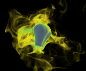The gas with high diffusivity (${Sc}=1$) has thicker boundary layers (figure 4(c,d) compared to the low-diffusivity gas (${Sc}=10$; figure 4e,f) subjected to the exact same flow. Figure 5 shows a three-dimensional rendering of the same times of the simulations, displaying the three-dimensional concentration field around the bubble, as the bubble moves in the flow, with lower ${Sc}=1$ in figure 5(a,b) and higher ${Sc}=10$ in figure 5(c,d). Again, higher Schmidt numbers lead to thinner boundary layers around the bubble for the same flow field.

Figure 4. Mass diffusion from the bubble in turbulence at two different times, $(t-t_0)/t_c=1.5$ (a,c,e) and 2 (b,d,f), showing a two-dimensional planar cut of the magnitude of the vorticity field (a,b) and concentration field for ${Re}_{\lambda }=77$, ${Sc}=1$ ($Pe^{(t)}=205$) (c,d) and ${Re}_{\lambda }=77$, ${Sc}=10$ ($Pe^{(t)}=2050$) (e,f). The wake in the vorticity field presents similarities to the structure of the concentration field. Higher Schmidt numbers lead to a thinner boundary layer around the bubble and a thinner wake structure.

Figure 5. three-dimensional rendering of the concentration field for $(t-t_0)/t_c=1.5$ (a,c) and 2 (b,d). (a,b) Concentration field for ${Re}_{\lambda }=77$, ${Sc}=1$ ($Pe^{(t)}=205$) and (c,d) concentration field for ${Re}_{\lambda }=77$, ${Sc}=10$ (${Pe}^{(t)}=2050$). Thinner boundary layers are observed at higher Schmidt numbers.

We next compute the total transfer rates $k_L$ of gases corresponding to increasing Schmidt numbers, and show their evolution with time in figure 6 for increasing numerical resolution: $d_0/\Delta x=136$ points per bubble diameter (figure 6a,b) and $d_0/\Delta x=273$ points per bubble diameter (figure 6c,d); and increasing turbulence Reynolds number: ${Re}_\lambda =38$ (figure 6a,c) and ${Re}_{\lambda }=77$ (figure 6b,d). The time is shifted to the bubble insertion time $t_0$ and normalized with the eddy turnover time $t_c$. After a short transient, the transfer rates reach a steady state for $(t-t_0)/t_c>0.25$. The transfer rates in steady state are compared with the predicted rates given by (2.3), which are shown as dashed lines. At lower resolution and Reynolds number (figure 6a; $d_0/\Delta x=136$ and ${Re}_\lambda =38$), all cases exhibit good agreement between computed and predicted transfer rates, and results are unchanged when the resolution is increased (see figure 6c; $d_0/\Delta x=273$ and ${Re}_\lambda =38$). The decrease in rates over time for lower-Schmidt-number cases in figure 6(a,b) is due to a considerable decrease in concentration of the transferred dilute gas. When increasing the Reynolds number, higher resolution is required for the highest Schmidt numbers, as visible in figure 6(b,c). To summarize, the DNS results are in close agreement with the predicted rates for $50<\widetilde {{Pe}}<10^{4}$, with $\widetilde {{Pe}}={u_{{rms}}d_0}/{\mathscr {D}_l}$ the turbulent Péclet number.

Figure 6. Non-dimensional mass transfer rates ${Sh}$ as a function of time, as the bubble is exposed to the turbulent flow. (a,b) Lower resolution $d_0/\Delta x=136$ (level 10), for ${Re}_{\lambda } = 38$ (a) and ${Re}_{\lambda } = 77$ (b). (c,d) Higher resolution (solid line for level 11 $d_0/\Delta x=273$, dotted line for level 12 $d_0/\Delta x=546$), for ${Re}_{\lambda } = 38$ (c) and ${Re}_{\lambda } = 77$ (d). Dashed lines represent the theoretical prediction (2.3) for the different Schmidt numbers. At steady state, very good agreement between simulations and theory is achieved for $\widetilde {{Pe}}={u_{{rms}}d_0}/{\mathscr {D}_l}={Sc} (u_{{rms}} d_0/\mathscr {D}_l)\leqslant 10^{4}$, which corresponds to a diffusive boundary layer $\delta _{k}$ resolved with more than approximately four grid points.

For higher turbulent Péclet numbers ($1.02\times 10^{4},\; 2.05\times 10^{4}$), we observe an overprediction of transfer rates. These results for the cases of $\widetilde {{Pe}}>10^{4}$ (yellow and black curves in figure 6b,d) can be understood by considering the resolution of boundary layers. The thickness of the hydrodynamic boundary layer $\delta _\nu$ around a spherical bubble is of ${\textit{O}}({Re}^{-1/2})$ (Moore Reference Moore1963). The concentration boundary layer thickness $\delta _k \propto \delta _\nu \,{Sc}^{-1/2}$ (Levich Reference Levich1962; Bothe & Fleckenstein Reference Bothe and Fleckenstein2013) scales with the bubble diameter $d_0$, and is given by ${\delta _k}/{d_0} \approx {Pe}^{-1/2}$. The numerical framework used in the present work uses adaptive mesh refinement with respect to the norm of the second-derivative of velocity and concentration (van Hooft et al. Reference van Hooft, Popinet, van Heerwaarden, van der Linden, de Roode and van de Wiel2018), with an error threshold of $0.2$ times the average of fields over the entire domain. The average of concentration fields is very small as most of the domain has trace amounts of gas concentration. This leads to a resolution of the boundary layers ranging from 40 grid points ($\widetilde {{Pe}}\approx 50, \delta _\nu /d_0\approx 0.13,\delta _k/d_0\approx 0.13$) to 3 grid points ($\widetilde {{Pe}}\approx 2 \times 10^{4},\delta _\nu /d_0\approx 0.07,\delta _k/d_0\approx 0.007$). When the resolution is increased, we are able to resolve thinner boundary layers, hence higher Péclet numbers ($1.02\times 10^{4}, 2.05\times 10^{4}$), as shown in figures 6(b) and 6(d) where the rates for $\widetilde {{Pe}}>10^{4}$ are converging to the predicted value as the resolution increases (L11 in solid lines and L12 in dotted lines).

Finally, figure 7 shows the Sherwood numbers obtained from the bubble mass transfer in homogeneous and isotropic turbulence simulations for a wide range of turbulent Péclet numbers ($50 < \widetilde {{Pe}} \leqslant 2\times 10^{4}$) for three different resolutions (simulation conditions are summarized in table 2). Very good agreement is observed between (2.3), up to $\widetilde {{Pe}} \sim 10^{4}$. As such, figure 7 validates (2.3), which predicts the transfer rates from the bubble in homogeneous and isotropic turbulent flow. We note that for ${Pe}\approx 2 \times 10^{4}$, an effective resolution L12 brings the simulated transfer rate closer to our theoretical prediction, as a result of increased resolution in the turbulent–diffusive boundary layer next to the bubble interface. We recall that figure 7 shows the scaling for the transfer rate $k_L$, as the non-dimensional Sherwood number, which reads $Sh \propto {Re}^{0.5}{Sc}^{0.5} = \sqrt {\widetilde {{Pe}}}$, and considering the definition of the Sherwood number, this corresponds to $k_L \propto {Sc}^{-0.5}\sqrt {{u_{{rms}}\nu _l}/{d_0}}$.

Figure 7. The transfer rates (for $(t-t_0)/t_c\geqslant 0.2$) with respect to Péclet number. Symbols are for different ${Re}_{\lambda }$ and resolution. For $\widetilde {{Pe}}\leqslant 10^{4}$, the numerical results are grid converged (first order) between L10 and L11, and agree very well with the theoretical prediction (2.3), ${Sh}=2(3)^{1/4}\sqrt {\widetilde {{Pe}}/{\rm \pi} }$. For higher Péclet numbers ($1.02\times 10^{4}, 2.05\times 10^{4}$), higher resolutions may converge to the prediction as visible when using L12 simulations. The transfer rates from Dodd et al. (Reference Dodd, Mohaddes, Ferrante and Ihme2021) correspond to the transfer rates from simulations of an evaporating drop at early times and agree with our data and model.

We note that Dodd et al. (Reference Dodd, Mohaddes, Ferrante and Ihme2021) present simulations of a droplet evaporating in turbulence and their evaporation rates at early times before significant volume change has occurred are in agreement with our model, as shown in figure 7.

The computed Sherwood numbers show convergence to the predicted value as the grid resolution increases. For the thinner boundary layers, corresponding to ${Re}_\lambda =77$ and high Schmidt number at $d_0/\Delta x=273$ resolution, the total number of cells in the domain reached 27.5 million and used $2.16\times 10^{4}$ CPU hours for $0.5$ eddy turnover time when the transfer rates approach a steady state. A corresponding constant-resolution DNS would have required $(2^{11})^{3} \approx 8.6$ billion cells, which illustrates the gain in efficiency brought by adaptive mesh refinement. It highlights the potential of adaptive mesh refinement methods for complex two-phase flows at high Péclet number, complementary to subgrid-scale modelling approaches.

We note that in § 2, we proposed the large-scale velocity fluctuations as the controlling velocity scale. As already mentioned, another choice could have been the velocity fluctuations at the scale of the bubble. Such a choice would not have changed the results obtained in figure 7, as these velocities are similar at the Reynolds number at the Taylor scale we consider.

Finally let us comment that at high Reynolds numbers, in the case of a flat interface, the scaling of the gas transfer is shifted from $Re^{1/2}$ to $Re^{3/4}$ due to the role of small eddies in enhancing the gas exchange (Theofanous et al. Reference Theofanous, Houze and Brumfield1976; Herlina & Wissink Reference Herlina and Wissink2016). Whether such a regime could be observed in the case of bubble mass exchange at high Péclet or Reynolds number remains to be investigated.