Introduction
The crocodile shark, Pseudocarcharias kamoharai, is a small-sized oceanic pelagic shark belonging to the order Lamniformes. It is the smallest lamniform species with a size at birth of around 41 cm total length (Oliveira et al., Reference Oliveira, Hazin, Carvalho, Rego, Coelho, Piercy and Burgess2010) and the only species of the family Pseudocarchariidae. The crocodile shark has an epipelagic and mesopelagic circumtropical distribution, it is usually found offshore and far from land but sometimes occurs inshore (Compagno, Reference Compagno2001). Vertically it can be distributed at depths from the surface to at least 590 m (Compagno, Reference Compagno2001). Despite being caught in tropical and sub-tropical waters in the Atlantic, Indian and Pacific oceans, the crocodile shark has an apparent unequal distribution, as in some regions it is quite rare while in others can be relatively abundant (Compagno, Reference Compagno2001).
Pseudocarcharias kamoharai is occasionally caught as by-catch by longliners targeting tuna and swordfish (Hazin et al., Reference Hazin, Couto, Kihara, Otsuka and Ishino1990). In the Portuguese longline fishery, the crocodile shark is more captured in some of the fishing areas, such as around the Cabo Verde archipelago and in the Gulf of Guinea, albeit in much lower numbers than the blue shark (Prionace glauca) (Coelho et al., Reference Coelho, Fernandez-Carvalho, Lino and Santos2012). Caught individuals are usually discarded, dead or alive, due to its lack of commercial value (Oliveira et al., Reference Oliveira, Hazin, Carvalho, Rego, Coelho, Piercy and Burgess2010). Therefore, this species is not accounted for in the official fisheries landings statistics, limiting the availability of data for monitoring its fisheries mortality and assessing its population status.
Elasmobranchs are, in general, highly susceptible to overexploitation due to their life history characteristics (Stevens et al., Reference Stevens, Bonfil, Dulvy and Walker2000). Lamniform sharks are even more susceptible due to their low fecundity, and specifically in the crocodile shark usually only four individuals are born per female in each reproductive cycle (Oliveira et al., Reference Oliveira, Hazin, Carvalho, Rego, Coelho, Piercy and Burgess2010; Dai et al., Reference Dai, Zhu, Chen, Xu and Chen2012). The crocodile shark is globally listed as ‘Least Concern’ by the IUCN Red List criteria (Kyne et al., Reference Kyne, Romanov, Barreto, Carlson, Fernando, Fordham, Francis, Jabado, Liu, Marshall, Pacoureau and Sherley2019), however it is noted that catch rates and population trends should continue to be monitored due to its vulnerability as by-catch in longline fisheries and due to its life history traits (Kyne et al., Reference Kyne, Romanov, Barreto, Carlson, Fernando, Fordham, Francis, Jabado, Liu, Marshall, Pacoureau and Sherley2019). In 2012, Cortés et al. (Reference Cortés, Domingo, Miller, Forselledo, Mas, Arocha, Camapana, Coelho, Da Silva, Hazin, Holtzhausen, Keene, Lucena, Ramirez, Santos, Semba-Murakami and Yokawa2015) conducted an ecological risk assessment (ERA) for several elasmobranch species in the Atlantic, and while the crocodile shark was initially considered for this analysis, the lack of biological data hampered the assessment.
A few studies of crocodile shark reproduction have been carried out in the Pacific (Fujita, Reference Fujita1981; Dai et al., Reference Dai, Zhu, Chen, Xu and Chen2012), Indian (White, Reference White2007) and Atlantic (Oliveira et al., Reference Oliveira, Hazin, Carvalho, Rego, Coelho, Piercy and Burgess2010; Wu et al., Reference Wu, Kindong, Dai, Sarr, Zhu, Tian, Li and Nsangue2020) oceans. Since the Cortés et al. (Reference Cortés, Domingo, Miller, Forselledo, Mas, Arocha, Camapana, Coelho, Da Silva, Hazin, Holtzhausen, Keene, Lucena, Ramirez, Santos, Semba-Murakami and Yokawa2015) ERA, two age and growth studies have become available for this species in the Atlantic Ocean (Lessa et al., Reference Lessa, Andrade, De Lima and Santana2016; Kindong et al., Reference Kindong, Wang, Wu, Dai and Tian2020). Age and growth studies are fundamental to estimate population growth rates, natural mortality, and longevity of a species (Campana, Reference Campana2001).
To add to the knowledge of the vital life-history parameters of this species, the objectives of this work were to study various aspects of the life history parameters of P. kamoharai, specifically growth, maturity and fecundity. The results presented here will be useful for modelling purposes (e.g. risk analysis) and may serve as a basis for comparison with other studies on this species, both in the Atlantic as well as in other oceans.
Materials and methods
Biological samples
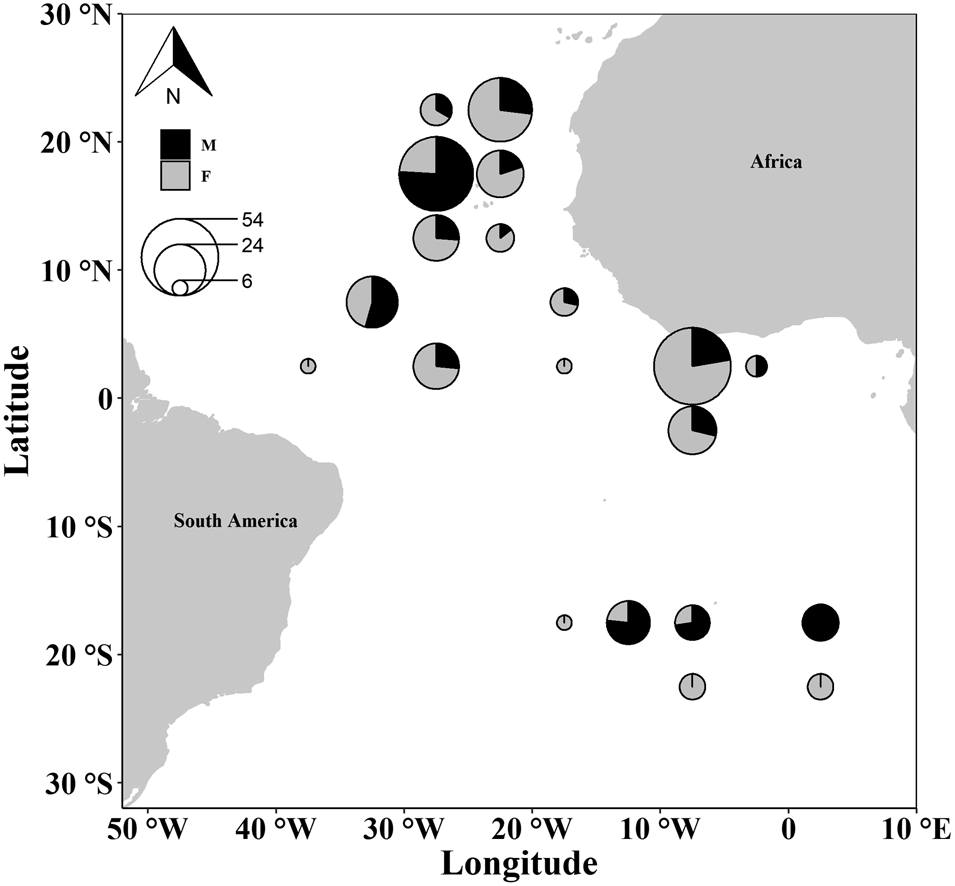
Specimens were obtained by observers from the Portuguese Institute for the Ocean and Atmosphere (IPMA, I.P.) on board Portuguese commercial longline vessels targeting swordfish between 2009 and 2012. Samples were collected over a wide Atlantic region (latitudes 25°N to 25°S; longitudes 7°E to 40°W) (Figure 1).

Fig. 1. Map of the Atlantic areas with the sampling locations of the crocodile shark (Pseudocarcharias kamoharai). The circles are represented in a 5° × 5° grid, with the sizes of the circles proportional to sample size and colour representing sex.
All specimens caught were frozen onboard, brought to the laboratory and processed shortly after. Each specimen was sexed, and a series of external body measurements were taken to the nearest lower centimetre, namely the total length (TL), measured in a straight line from the tip of the snout to the tip of the caudal fin in its natural position, the fork length (FL), measured from the tip of the snout to the caudal fin fork, and the pre-caudal length (PCL), measured from the tip of the snout to the beginning of the upper lobe of the caudal fin. Total weight (W) and eviscerated weight (Wev) were recorded to the nearest centigram. After dissection, the liver was weighed to the nearest centigram. For females, the oviducal glands and uteri were measured for width and the ovary measured for width and length and weighed. Following dissection, the contents of the uteri were observed, and any developing embryos were counted and sexed. For males, the testes were measured for width and length, and weighed, the claspers were measured for inner and outer length and the presence of semen in the seminal glands recorded. All organs were measured to the nearest 0.1 mm using a digital calliper and weighed on a digital scale with a 0.01 g precision. The sex ratio of the samples was calculated and tested for equal proportions with a chi-square test.
Morphometric relationships
The length-length relationships between TL, PCL and FL and the length-weight relationship between FL, W and Wev without any data transformation, and the weight-weight relationship between W and Wev (in g) with natural logarithm transformed data were explored by linear regression. Standard errors were calculated for all the estimated parameters, along with the coefficient of determination (r 2) of each regression. Linear regressions were carried out to compare the main effects of the explanatory variable and sex and the interaction term between the explanatory variable and sex.
Age estimation and validation
A section of 3–5 vertebrae was extracted from the region below the anterior part of the first dorsal fin. The covering of connective tissue on the vertebrae was first removed with scalpels, and then by soaking the vertebrae in 4–6% sodium hypochlorite (commercial bleach) for 5 to 10 min, depending on size. Once cleaned, the vertebrae were stored in 70% ethanol and then air-dried for 24 h before embedding in polyester resin, in individual plastic moulds, and left to harden for ~24 h.
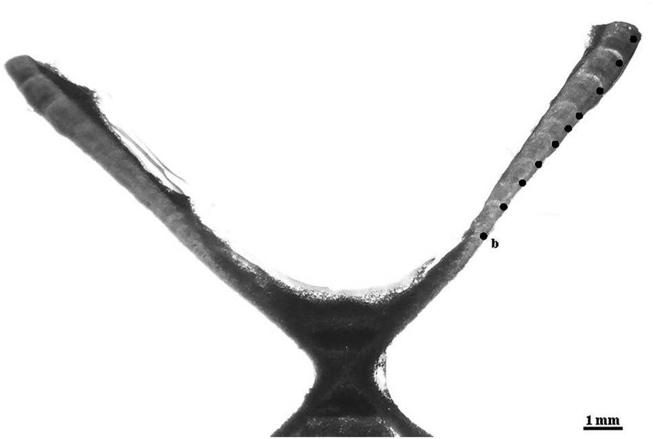
The resin blocks with the embedded vertebrae were sectioned sagittally with a Buehler Isomet (Lake Bluff, IL) low-speed saw, using two blades spaced ~500 μm apart. The resulting section included the focus of the vertebra and the two halves (one on each side of the focus), in a form typically called ‘bow-tie’. Finally, the sections were stained with crystal violet (Sigma-Aldrich Co., St. Louis, MO). Once dried, the sections were mounted onto microscope slides with Cytoseal 60 (Thermo Fisher Scientific Inc., Waltham, MA). The visualization of the vertebral sections was carried out under a dissecting microscope using transmitted white light (Figure 2).

Fig. 2. Microphotograph of a vertebral section of the crocodile shark (Pseudocarcharias kamoharai), from a female specimen with 80 cm fork length with the identification of the birth mark (b) and the estimated nine growth bands.
Sections from the same specimen were read once by two different readers. Counts were made with no knowledge of the sex or size of the individual. Whenever band pair counts differed between the two readers by one or two band pairs, a third reading was made. If disagreement between readings persisted or if the band pair count between readers disagreed by three or more band pairs, the section was discarded. The precision of the age estimates was determined by several different techniques. The per cent agreement (PA), the average per cent error (APE) defined by Beamish & Fournier (Reference Beamish and Fournier1981) and the coefficient of variation (CV) were used. Bias plots were used to graphically assess the ageing accuracy between the readers (Campana, Reference Campana2001). Precision analysis was carried out using the R language for statistical computing version 3.6.1 (R Core Team, 2019), using the package ‘FSA’ (Ogle et al., Reference Ogle, Wheeler and Dinno2020). All plots were performed using package ‘ggplot2’ (Wickham, Reference Wickham2016).
Growth modelling
The relationship between the size of the specimens and the size of their vertebrae was determined. The vertebral sections were photographed using a dissecting microscope and the vertebral radius of the vertebrae was digitally measured using Image J software (Abramoff et al., Reference Abramoff, Magalhaes and Ram2004). A linear and a quadratic regression was fitted using FL as the dependent variable and the vertebral radius (VR) as the independent variable. Model comparison was based on Akaike information criterion (AIC) and Bayesian information criterion (BIC) and the coefficient of determination (r 2), where the model with the lowest AIC/BIC and highest r 2 was considered the model that best fitted the data and described the FL-VR relationship.
To verify the temporal periodicity of band formation in the vertebral centra, an edge analysis and a marginal increment analysis was initially attempted. However, due to the lack of captures for each month and for every estimated age class, it was not possible to determine the periodicity of band formation. The deposition of a band pair (one translucent and one opaque band) per year was assumed (see Discussion section for details).
Five models were used to describe this species’ growth. The 3-parameter von Bertalanffy growth function (VBGF) re-parameterized to estimate L 0 (size at birth) instead of t 0 (theoretical age at which the expected length is zero), as suggested by Cailliet et al. (Reference Cailliet, Smith, Mollet and Goldman2006):
 $$L_{\rm t} = L_{\inf }-( L_{\inf }-L_0) \times \exp ^{( {-k_1 \times t} ) }$$
A 2-parameter VBGF where L 0 was fixed to the size at birth described for this species was also used.
The Gompertz growth function (GOM):
 $$L_{\rm t} = L_{\inf } \times \exp ^{( {-}a \times {\exp }^{( {-k_2 \times t} ) }) }$$
The logistic model (LOG):
 $$L_{\rm t} = \displaystyle{{L_{\inf }} \over {1 + {\exp }^{( {-k_3 \times ( t-t_{\rm i}) } ) }}}$$
Finally, a Richards model (RICH) re-parameterized to estimate L 0 was also used, with a fixed L 0 at the size at birth described for this species:
 $$L_{\rm t} = L_{\inf } \times \left({1 + \left({{\displaystyle{{L_0} \over {L_{\inf }}}}^{( 1-b) }-1} \right)\times \;{\exp }^{( {-}k_4 \times t) }} \right)^{( {1/( 1-b) } ) }$$
where L t = mean fork length at age t; L inf = mean asymptotic fork length; k 1 = relative growth coefficient; L 0 = fork length at birth, k 2 = instantaneous growth rate at the inflection point; a = dimensionless parameter related to growth; k 3 = instantaneous growth rate at negative infinity; t i = time at the inflection point, k 4 = controls the slope at the inflection point; b = a dimensionless parameter that controls the vertical position of the inflection point.
For the models with fixed L 0, because size data in our study refer to FL, the size at birth from Oliveira et al. (Reference Oliveira, Hazin, Carvalho, Rego, Coelho, Piercy and Burgess2010) of 41 cm TL was converted using the TL-FL relationship in Table 1, resulting in 32 cm FL.
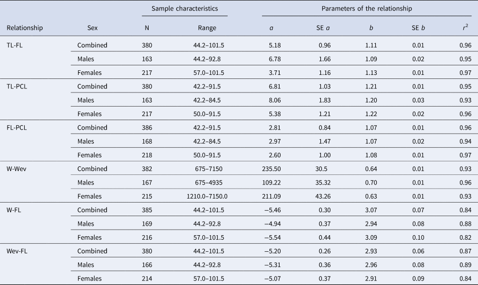
Table 1. Morphometric relationships for crocodile shark (Pseudocarcharias kamoharai) collected in the tropical Atlantic Ocean

For each model, parameters are presented with the respective standard errors (SE) and the coefficient of determination (r 2). TL = total length (cm), FL = fork length (cm), PCL = pre-caudal length (cm), W = total weight (g), Wev = Eviscerated weight (g). Range is in centimetres for the length-length and length-weight relationships, and in grams for the weight-weight relationship. Length-length and weight-weight relationships do not have any transformation while length-weight relationships are log transformed.
Model comparison was based on AIC and BIC. Growth models were fitted using non-linear least squares function from the ‘minpack.lm’ package (Elzhov et al., Reference Elzhov, Mullen, Spiess and Bolker2016) in R (R Core Team, 2019). A likelihood ratio test (LRT) was used to test the null hypothesis that there was no difference in growth parameters between males and females.
Maturity and fecundity
Maturity was assigned by macroscopically observing the condition of the reproductive system. Following Oliveira et al. (Reference Oliveira, Hazin, Carvalho, Rego, Coelho, Piercy and Burgess2010), for males, maturity was assigned based on the calcification and size of the claspers; for females, maturity was assigned based on the presence of uterine contents and the dimensions of the reproductive organs such as the ovary, oviducal glands, and uterus. For paired structures, both the left- and the right-side structures were measured and tested for normality with Kolmogorov–Smirnov normality tests with the Lilliefors correction (Lilliefors, Reference Lilliefors1967), and for homogeneity of variances with Levene tests (Levene, Reference Levene, Olkin, Ghurye, Hoeffding, Madow and Mann1960). Dimensions of the structures was compared among left and right side using non-parametric 2-sample permutation tests (Manly, Reference Manly2007). Each structure dimension, for each male and female, was plotted against FL so that relative growth of the structure with size could be observed (Supplementary material).
The gonadosomatic index (GSI) and the hepatosomatic index (HSI) were calculated as:
 $${\rm GSI} = \displaystyle{{{\rm Gonad}\;{\rm weight}( {\rm g}) } \over {{\rm Wev}( {\rm g}) }} \times 100$$
 $${\rm HSI} = \displaystyle{{{\rm Liver}\,{\rm weight}( {\rm g}) } \over {{\rm Wev}( {\rm g}) }} \times 100$$
For males, gonad weight was calculated as the sum of left and right testis weight, for females the ovary weight was used. GSI and HSI was tested for normality with Kolmogorov–Smirnov normality tests with the Lilliefors correction (Lilliefors, Reference Lilliefors1967), and for homogeneity of variances with Levene tests (Levene, Reference Levene, Olkin, Ghurye, Hoeffding, Madow and Mann1960). To test for differences in GSI and HSI between mature and immature specimens, ANOVA tests were performed. When the assumptions of parametric tests were not met, non-parametric 2-sample permutation tests (Manly, Reference Manly2007) were used. A plot of HSI and GSI for mature specimens was produced for visual inspection of the monthly trends in these indices.
Raw maturity data were used to fit length-based maturity ogives and to estimate the size at 50% maturity (L 50, FL at which 50% of the individuals are mature). A logistic regression was fit by GLM with a binomial response variable, using the ‘glm’ function in R (R Core Team, 2019). The predicted probability of an individual being mature at a given length is given by:
 $$P_{L_i} = \displaystyle{{{\exp }^{( \alpha + \beta \times L_i) }} \over {1 + {\exp }^{( \alpha + \beta \times L_i) }}}$$
where PLi is the probability of an individual being mature at length i, α the intercept term and β the effect size in terms of length.
The same procedure was followed to fit age-based maturity ogives and estimate age at maturity (A 50, age at which 50% of the individuals are mature). The predicted probability of an individual being mature at a given age is given using the equation:
 $$P_{{\rm Ag}{\rm e}_i} = \displaystyle{{{\exp }^{( {\alpha + \beta \times {\rm Ag}{\rm e}_i} ) }} \over {1 + {\exp }^{( {\alpha + \beta \times {\rm Ag}{\rm e}_i} ) }}}$$
where P Agei is the probability of an individual being mature at age i, α the intercept term and β the effect size in terms of age.
The inflection points of the relationships represent L 50 and A 50, where P = 0.5, these values were calculated and 95% confidence intervals (CI) obtained through bootstrapping from binomial GLM fits to 1000 resamples of the maturity data using the ‘boot’ package (Canty & Ripley, Reference Canty and Ripley2019). Length and age-based maturity ogives were fitted to males and females separately, and an LRT used to test for differences between sexes.
Fecundity was estimated by direct methods, by counting the number of mid-term embryos in pregnant females. Numbers of developing embryos occurring in the left and right uteri were compared with a Mann–Whitney U-test (given that the samples were not normally distributed). The sex ratio of the embryos was calculated and tested for equal proportions with a chi-square test.
Results
Biological samples
A total of 391 specimens (220 females and 171 males) was caught for this study during the sampling period. The sex ratio of the samples significantly favoured females (two proportion z-test, n females = 220, n males = 171, χ2 = 12.28, P < 0.001). Of these samples, 358 specimens were used for the age and growth study and 387 specimens for the maturity component. Both male and female samples had a wide length range (Figure 3), covering most of the length range described for this species. Females attained slightly larger sizes than males. Specifically, female lengths varied from 57.0–101.5 cm FL while males ranged from 44.2–92.8 cm FL (Figure 3). Males ranged in total weight from 675–5120 g and females from 1210–7425 g.
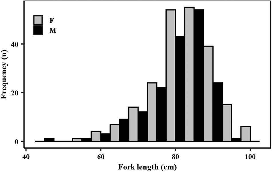
Fig. 3. Length (fork length, in 5 cm length bins) frequency distribution of male (N = 171) and female (N = 220) crocodile shark (Pseudocarcharias kamoharai), collected in the tropical Atlantic Ocean.
Morphometric relationships
The morphometric relationships for P. kamoharai are presented in Table 1. For the TL-FL relationship the interaction term between FL and sex was not significant and no significant differences between sexes were detected (ANOVAFL:Sex: F = 2.02, P > 0.05; ANOVASex: F = 2.09, P > 0.05). For TL-PCL there is not a significant interaction term between PCL and sex (ANOVAPCL:Sex: F = 1.12, P > 0.05) but significant differences were found for sex (ANOVASex: F = 4.33, P < 0.05), this means that the slope of the regression curve is not significantly different between the sexes, but the intercept between sexes is different. For the FL-PCL relationship, the interaction term between PCL and sex was not significant and no significant differences between sexes were detected (ANOVAPCL:Sex: F = 0.03, P > 0.05; ANOVASex: F = 0.21, P > 0.05).
For the W-Wev regression a significant interaction was found between Wev and sex and significant differences were detected between sexes (W-Wev: ANOVAWev:Sex: F = 14.78, P < 0.001; ANOVASex: F = 43.99, P < 0.001). For W-FL the interaction term between FL and sex was not significant but significant differences between sexes were detected (ANOVATL:Sex: F = 1.30, P > 0.05; ANOVASex: F = 25.69, P < 0.001), whereby females are significantly heavier than males for a given length. For Wev-FL the interaction term between FL and sex was not significant and no significant differences between sexes were detected (ANOVAFL:Sex: F = 0.19, P > 0.05; ANOVASex: F = 0.91, P > 0.05).
Age estimation and growth modelling
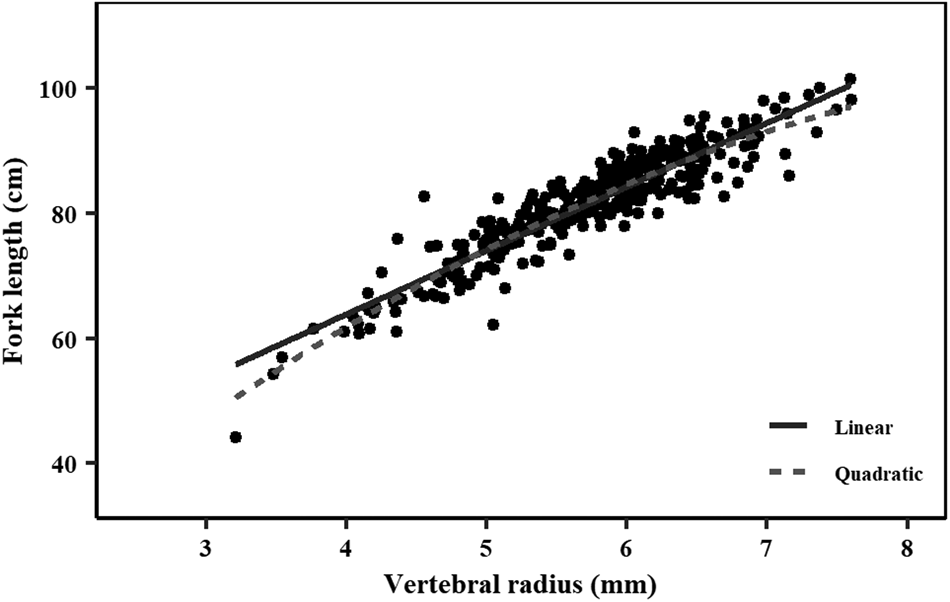
There was a slight curvilinear relationship between VR and FL (Figure 4). A linear regression had a good fit to the data (FL = 23.03 + 10.20 × VR; r 2 = 0.85; AIC = 1830; BIC = 1842); however, the quadratic equation produced a slightly better goodness-of-fit (FL = 21.75 × VR–1.03 × VR2−8.76; r 2 = 0.86; AIC = 1806; BIC = 1822). Inter-specific CV and APE were 5.61% and 3.97%, respectively. PA between the first and second reader was 48.01%, while the PA within one and two band pairs was 89.49% and 97.73%, respectively. A high agreement with no systematic bias was observed between the readings of the two readers using the age-bias plots (Figure 5).

Fig. 4. Relationship between fork length (cm) and vertebrae centrum radius (mm) for crocodile shark (Pseudocarcharias kamoharai) collected in the tropical Atlantic Ocean. Dots represent individual observations. Solid line represents linear regression where: FL = 23.03 + 10.20 × VR. Dashed line represents quadratic regression where: FL = 21.75 × VR – 1.03 × VR2 – 8.76. FL = fork length; VR = vertebral radius.
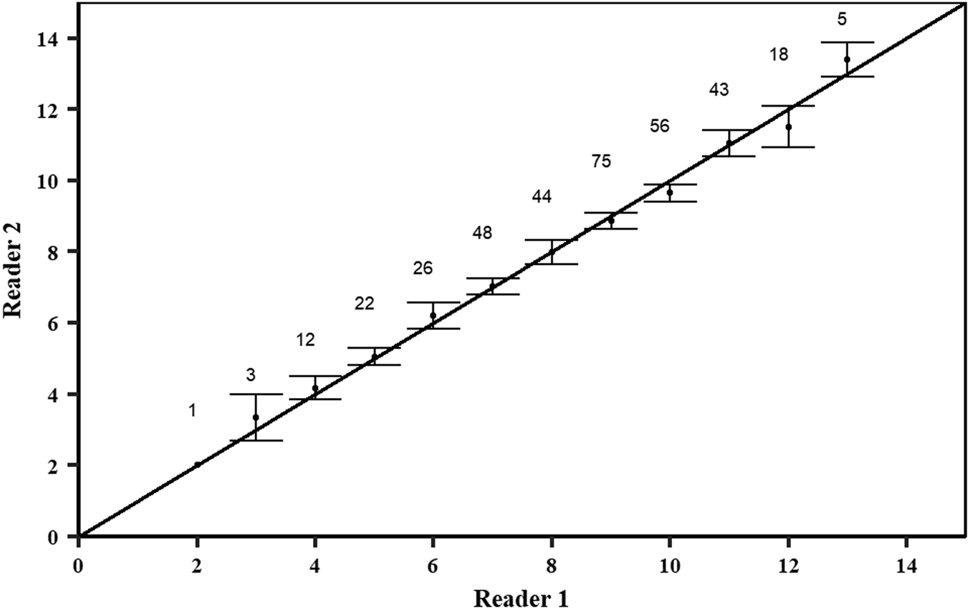
Fig. 5. Age–bias plots of pairwise growth band counts comparisons between reader 1 and reader 2. Numbers represent number of samples and dots with error bars represent the mean counts of reading (± 95% confidence intervals) relative to the accepted growth band count. The diagonal line indicates a one-to-one relationship.
A total of 338 (94.41%) vertebrae had a final agreed band pair count and thus were accepted for growth modelling. Fork lengths of individuals with an agreed band pair count ranged from 57.0–100.0 cm and 44.2–92.8 cm FL for females and males, respectively. Estimated ages of the analysed specimens ranged from 3–14 years for females and from 2–13 years for males. The LRT revealed significant differences between males and females for all growth models (LRT; 3-parameter VBGF: χ2 = 32.06, df = 3, P < 0.001; 2-parameter VBGF: χ2 = 31.15, df = 2, P < 0.001; GOM: χ2 = 32.02, df = 3, P < 0.001; LOG: χ2 = 31.95, df = 3, P < 0.001; RICH: χ2 = 31.94, df = 3, P < 0.001), therefore growth models were calculated for each sex separately.
All five models produced very similar curves, both in the case of males and females (Figure 6). AIC values were similar, despite VBGF with a fixed L 0 having the lowest AIC, for both females and males, BIC presents the same tendency, with differences between the VBGF with a fixed L 0 being larger than for AIC (Table 2). In general, the differences between the AIC/BIC values are small, indicating that there is little statistical difference between the models.
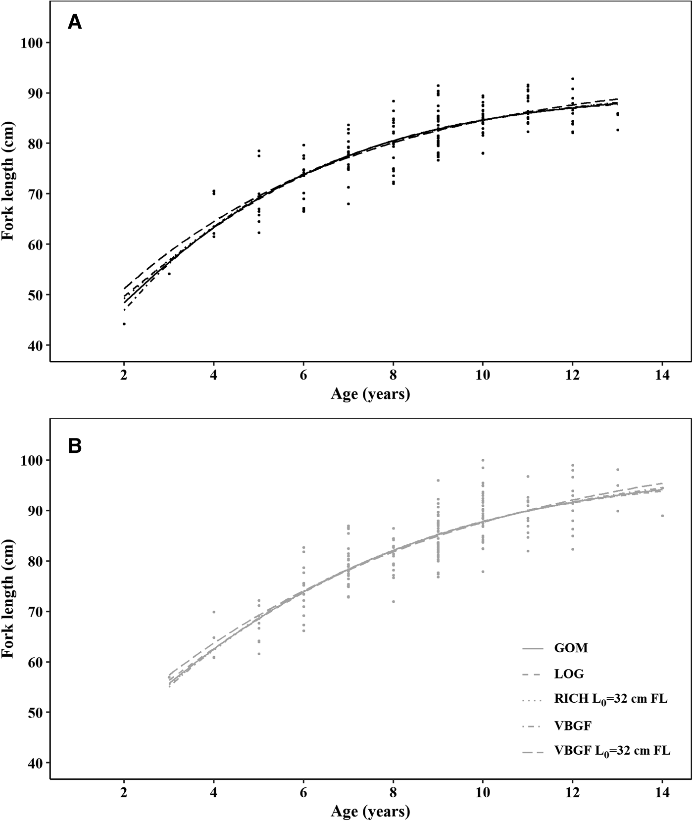
Fig. 6. Growth functions for (A) males and (B) females crocodile shark (Pseudocarcharias kamoharai) in the tropical Atlantic, based on growth band counts in vertebral sections. Circles represent observed data and lines represent the fitted models. VBGF stands for the von Bertalanffy growth function, VBGF L 0 = 32 cm FL for the VBGF with fixed size at birth at 32 cm fork length GOM for the Gompertz model, LOG for the logistic model and RICH L 0 = 32 cm FL for the Richards model with fixed size at birth at 32 cm fork length.
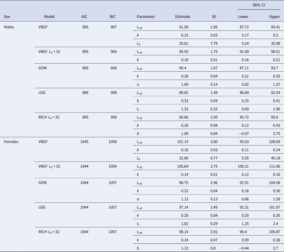
Table 2. Growth parameters for crocodile shark (Pseudocarcharias kamoharai) from the tropical Atlantic Ocean, fitted with individual observed data

The presented models are the re-parameterized von Bertalanffy growth function (VBGF), the VBGF with fixed L 0 at 32 cm fork length (FL), the Gompertz growth function (GOM), the logistic model (LOG) and the Richards model (RICH) with fixed L 0 at 32 cm. For each model, parameters are presented with the respective standard errors (SE) and 95% confidence intervals (CI). L inf = mean asymptotic length (cm FL), k 1 = relative growth coefficient (year−1), L 0 = size at birth (cm FL), k 2 = instantaneous growth rate at the inflection point (year−1); a = dimensionless parameter related to growth; k 3 = instantaneous growth rate at negative infinity (year−1); t i = time at the inflection point (year), k 4 = controls the slope at the inflection point (year−1); b = a dimensionless parameter that controls the vertical position of the inflection point.
In all models, females had higher maximum asymptotic sizes than males. The logistic equation produced the lowest maximum asymptotic lengths and the VBGF with a fixed L 0 the highest values, inversely the estimated growth coefficients were lower for the VBGF with a fixed L 0 and highest for the logistic model (Table 2, Figure 6). The VBGF estimated L 0 of 20.6 cm FL for males and 22.9 cm FL for females are smaller than the reported size at birth for this species.
Maturity and fecundity
In the case of males, HSI data were not normally distributed (Lilliefors test: D = 0.09, P < 0.001), but the variances were homogeneous between mature and immature individuals (Levene test: F = 0.19, df = 1, P > 0.05). Using univariate non-parametric statistical tests revealed that HSI did not differ significantly between mature and immature individuals (permutation test: Z = 1.13, P > 0.05; Figure 7). GSI data were not normally distributed (Lilliefors test: D = 0.12, P < 0.001), and the variances were heterogeneous between mature and immature individuals (Levene test: F = 12.34, df = 1, P < 0.001). Using univariate non-parametric statistical tests revealed that GSI did not differ significantly between mature and immature individuals (permutation test: Z = 0.25, P > 0.05; Figure 7). For females, HSI data were normally distributed (Lilliefors test: D = 0.05, P > 0.05), and the variances were homogeneous between mature and immature individuals (Levene test: F = 0.45, df = 1, P > 0.05). Differences were found between stages for female HSI (ANOVA: F = 3.98, P < 0.05), with mature females having a higher HSI (Figure 7). GSI data were not normally distributed (Lilliefors test: D = 0.39, P < 0.001), and the variances were heterogeneous between mature and immature individuals (Levene test: F = 38.65, df = 1, P < 0.001). Using univariate non-parametric statistical tests revealed that GSI significantly differed between stages for females (permutation test: Z = 5.89, P < 0.001), with mature females having a higher GSI (Figure 7).
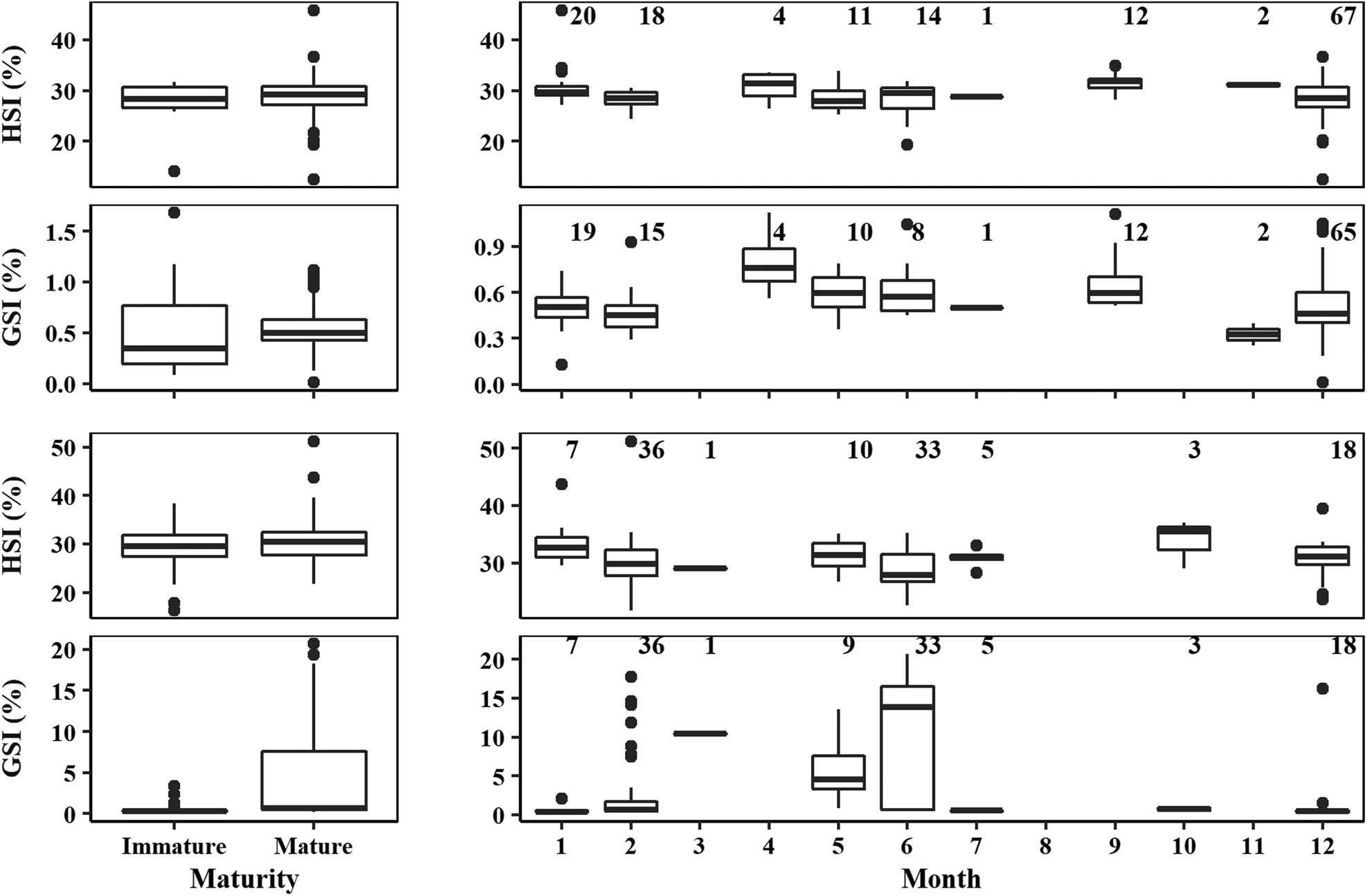
Fig. 7. Boxplot of the hepatosomatic index (HSI, %) and gonadosomatic index (GSI, %) between immature and mature specimens (left) and for mature specimens by month (right) for male (top) and female (bottom) crocodile shark (Pseudocarcharias kamoharai) in the tropical Atlantic Ocean. The box corresponds to the interquartile range (IQR, between the 25th and 75th percentiles), whiskers maximum and minimum represent the largest and lowest value, respectively, no further than 1.5*IQR, and dots represent data outside of this range.
Although with limited sample size by month and some missing months, a graphic representation of the HSI and GSI for mature specimens by month shows that there is low variation in HSI through the year for males (Figure 7) while for females there is a small decrease in the months where GSI is higher (Figure 7). For males, in the months from April to September the GSI also shows an increasing trend when compared with the other available months (Figure 7).
Immature males in the sample ranged from 44.2–77.6 cm FL, while mature males ranged from 62.2–92.8 cm FL, with 157 out of 169 (92.9%) of the males in the sample being mature. Immature females ranged from 57–93.7 cm FL, with the smallest mature female measuring 75.5 cm FL, and with 120 out of 218 (55.0%) of the females being mature. In terms of age, the youngest mature male was 4 years old, while the oldest immature male was 9 years old. Females matured at a later age, with the youngest mature female being 6 years old and the oldest immature female being 11 years old.
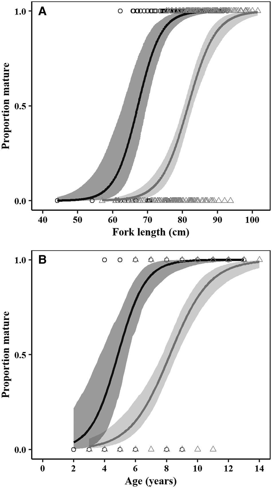
Females matured at larger sizes than males, with estimated L 50 of 81.57 cm FL for females and 67.20 cm FL for males (Figure 8, Table 3). Females also matured at later ages than males, with estimated A 50 of 4.85 years for males and 8.21 years for females (Figure 8, Table 3). There were significant differences between sexes in terms of the parameters of both length (LRT: χ2 = 149.88, df = 2, P < 0.05) and age-based (LRT: χ2 = 103.03, df = 2, P < 0.05) maturity ogives.

Fig. 8. (A) Size and (B) age-based maturity ogives for male (black) and female (grey) crocodile shark (Pseudocarcharias kamoharai), in the tropical Atlantic Ocean. Circles (○) and triangles (Δ) represent individual maturity data for males and females, respectively. The solid line represents the corresponding fitted logistic curve, while the shaded area represents the 95% confidence intervals.
Table 3. Size and age maturity ogive for crocodile shark (Pseudocarcharias kamoharai) from the tropical Atlantic Ocean, fitted with individual observed data
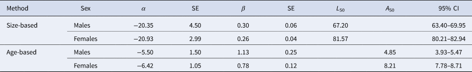
The values of α and β are the estimated parameters of the logistic function, SE is the standard error for the parameters, L 50 and A 50 is the length (cm) and age (years) at 50% maturity, respectively, and the 95% bootstrapped confidence intervals (CI)
Pregnant females were found in February, March, May, June and December, with most pregnancies occurring in May and June. Uterine fecundity varied from 2–4 embryos with a mean of 3.7 (SD = 0.6, n females = 34, n embryos = 123). No differences were found in the mean number of embryos counted in each uterus (Mann–Whitney U test, U = 580.5, n left = 61, n right = 62, P > 0.05). Most pregnant females had two embryos in each uterus, although 1 embryo per uterus (n = 3) and 2 in one uteri and 1 in the other (n = 3) was also found. The sex ratio of the embryos was close to 1:1, but slightly favoured females (53.2% females v. 46.8% males), although no significant statistical difference was detected (two proportion z-test, n females = 58, n males = 51, χ2 = 0.66, df = 1, P > 0.05). The most typical situation observed was for a pregnant female to have one male and one female embryo in each uterus, totalling two males and two females per reproductive cycle.
Discussion
Most of the known length range of the species was covered in the present study, namely with the lengths ranging from 44.2–101.5 cm FL, and with females attaining larger sizes than males. At the higher end, the larger individual in this study is close to the maximum reported length of 105Footnote 1 cm FL (122 cm TL; Lessa et al., Reference Lessa, Andrade, De Lima and Santana2016). Size at birth is reported to be between 36 and 45 cm TL according to White (Reference White2007), this range corresponds to 28–36 cm FL, which implies our study missed only the smallest individuals between the size at birth and 44.2 cm FL. Moreover, only a few samples were available below 60 cm FL. The lack of small individuals has also been reported in several studies focusing on crocodile shark life history (e.g. Oliveira et al., Reference Oliveira, Hazin, Carvalho, Rego, Coelho, Piercy and Burgess2010; Lessa et al., Reference Lessa, Andrade, De Lima and Santana2016; Kindong et al., Reference Kindong, Wang, Wu, Dai and Tian2020; Wu et al., Reference Wu, Kindong, Dai, Sarr, Zhu, Tian, Li and Nsangue2020). Oliveira et al. (Reference Oliveira, Hazin, Carvalho, Rego, Coelho, Piercy and Burgess2010) proposed that the absence of small individuals could be related to size selectivity of the gear or due to the absence of these individuals either due to different geographic distribution or different vertical distribution of the fishing gears compared with the distribution of those smaller specimens.
The sex ratio in the sample was significantly different from the expected 1:1, with more females in the catch as found by several authors (White, Reference White2007; Oliveira et al., Reference Oliveira, Hazin, Carvalho, Rego, Coelho, Piercy and Burgess2010; Dai et al., Reference Dai, Zhu, Chen, Xu and Chen2012; Lessa et al., Reference Lessa, Andrade, De Lima and Santana2016). On the contrary, some studies reported more males than females in fisheries catches (Ariz et al., Reference Ariz, Delgado de Molina, Ramos and Santana2006, Reference Ariz, Delgado de Molina, Ramos and Santana2007; Romanov et al., Reference Romanov, Ward, Levesque and Lawrence2008; Walsh et al., Reference Walsh, Bigelow and Sender2009; Kindong et al., Reference Kindong, Wang, Wu, Dai and Tian2020). The unbalanced sex ratios in different areas may indicate that fish aggregations can be spatially or temporally dependent (Dai et al., Reference Dai, Zhu, Chen, Xu and Chen2012). Sexual segregation and juvenile aggregations in specific areas might lead to a higher vulnerability of crocodile shark to commercial fisheries (Romanov et al., Reference Romanov, Ward, Levesque and Lawrence2008; Dai et al., Reference Dai, Zhu, Chen, Xu and Chen2012).
Regarding the precision of age readings, Campana (Reference Campana2001) mentions that precision is highly influenced by the species and the nature of the structure used, reporting that most ageing studies using vertebrae report a CV higher than 10%. In the current study, CVs were low and PA was high, especially within one band pair readings. The precision of age readings with the bias-plot graphics indicates that our age estimates were consistent.
An annual band-pair deposition rate was assumed in this study. An initial attempt to verify band pair deposition through marginal increment analysis was performed, however due to a heterogeneous sample size by month it was not possible to conduct this analysis. Lessa et al. (Reference Lessa, Andrade, De Lima and Santana2016) conducted a marginal increment analysis but results were inconclusive. Annual band pair deposition has been validated for other species of the same order, for example Alopias superciliosus (Liu et al., Reference Liu, Chiang and Chen1998), Alopias pelagicus (Liu et al., Reference Liu, Chen, Liao and Joung1999), Lamna nasus (Natanson et al., Reference Natanson, Mello and Campana2002) and Isurus oxyrinchus (Ardizzone et al., Reference Ardizzone, Cailliet, Natanson, Andrews, Kerr and Brown2006; Natanson et al., Reference Natanson, Kohler, Ardizzone, Cailliet, Wintner and Mollet2006). However, for shortfin mako other studies have validated a biannual deposition rate in juveniles (Wells et al., Reference Wells, Smith, Kohin, Freund, Spear and Ramon2013; Kinney et al., Reference Kinney, Wells and Kohin2016). A study of several species showed that band pair deposition may be more related with somatic growth and vertebrae size than to time or age (Natanson et al., Reference Natanson, Skomal, Hoffman, Porter, Goldman and Serra2018). Additionally, Harry (Reference Harry2018) alerts to the fact that many validation studies have reported underestimation in shark and ray ageing studies, especially in the larger and presumably older sharks. Ages can be underestimated if vertebrae cease to grow as maximum size is approached (Andrade et al., Reference Andrade, Rosa, Muñoz-Lechuga and Coelho2019), therefore estimated maximum ages in this study should be considered as low estimates of maximum age for this species. Age validation through a species' lifespan is of extreme importance, as incorrect age and growth parameters will influence longevity, mortality estimates and other biological processes, which are important input parameters for stock assessments and fisheries management (Goldman et al., Reference Goldman, Cailliet, Andrews, Natanson, Carrier, Musick and Heithaus2012; Cailliet, Reference Cailliet2015). Validation of band-pair deposition for P. kamoharai through its lifespan is lacking and should be considered in future studies.
In the present study, males and females reached different maximum sizes, but had similar maximum ages. The oldest estimated age was 13 years for males and 14 years for females. These estimates are older than the previous estimates by Lessa et al. (Reference Lessa, Andrade, De Lima and Santana2016) of 8 and 13 years for males and females, respectively, and Kindong et al. (Reference Kindong, Wang, Wu, Dai and Tian2020) of 11 years for males and 10 years for females. The differences in the maximum estimated age could be related to differences in population or sampled areas and sizes but could also be related to differences in vertebrae processing. According to da Silva Ferrette et al. (Reference da Silva Ferrette, Mendonça, Coelho, de Oliveira, Hazin, Romanov, Oliveira, Santos and Foresti2015) there is evidence for only one population in the Atlantic, and even between the Atlantic and the south-west Indian ocean, therefore differences can be due to the methodological aspects. The three available age and growth studies for crocodile shark have used different processing methods. In the current study vertebrae were sectioned and stained with crystal violet, while Lessa et al. (Reference Lessa, Andrade, De Lima and Santana2016) used unstained sections and Kindong et al. (Reference Kindong, Wang, Wu, Dai and Tian2020) used whole vertebrae stained with Alizarin Red S.
Contrary to the previous studies in age and growth for this species, that found no differences between males' and females' growth, in the present study differences were found between sexes, females having a higher L inf and lower growth coefficients than males, for all tested models. Growth is similar up until 6 years old, when the growth curves begin to separate. Taking into consideration that the statistical fit, assessed by AIC and BIC, was best for the 2-parameter VBGF, this model was chosen as the model that best represents growth for this species. Sampling for smaller/younger specimens (see discussion above regarding size range) could help improve the growth curve fit in the initial years, especially for the 3-parameter VBGF that underestimated L 0. It is noteworthy that other lamnoid sharks also present a lower L inf and higher k for males than females (e.g. Isurus oxyrinchus (Rosa et al., Reference Rosa, Mas, Mathers, Natanson, Domingo, Carlson and Coelho2017), Alopias superciliosus (Fernandez-Carvalho et al., Reference Fernandez-Carvalho, Coelho, Erzini and Santos2015a), Alopias vulpinus (Gervelis & Natanson, Reference Gervelis and Natanson2013)).
Regarding trends in HSI and GSI between mature and immature specimens, Oliveira et al. (Reference Oliveira, Hazin, Carvalho, Rego, Coelho, Piercy and Burgess2010) found that in males there was no difference in HSI between maturity stages, while GSI increased with maturity. In the present study, the small sample of immature males with high variance in GSI, without separation of juvenile and maturing specimens, could have hindered the assessment of a significant increase in GSI once males mature. For females, Oliveira et al. (Reference Oliveira, Hazin, Carvalho, Rego, Coelho, Piercy and Burgess2010) had a more detailed analysis into the different maturity stages and found that in the early stages of pregnancy there was an increase in HSI, while late-term pregnant females presented lower HSI, which recovered slightly in resting females. For GSI, the same authors observed that juvenile and resting female specimens had a low GSI, increasing in the initial pregnancy stages followed by a decrease towards late-term pregnancy. For the monthly analysis, the decrease in HSI in the months where GSI peaks, seems to agree with Oliveira et al. (Reference Oliveira, Hazin, Carvalho, Rego, Coelho, Piercy and Burgess2010) that noted a decrease in HSI through pregnancy, as females keep producing ova due to oophagy, spending high quantities of energy on this process. The same authors found all maturity stages throughout the year in females, with a peak in pregnant females occurring from May to July and juveniles in September and October. Both Oliveira et al. (Reference Oliveira, Hazin, Carvalho, Rego, Coelho, Piercy and Burgess2010) in the Atlantic Ocean and Fujita (Reference Fujita1981) in the Pacific Ocean suggest that crocodile shark might have a prolonged mating and parturition season.
Maturity estimates from Indonesia (White, Reference White2007) found males mature around 72.5 cm TL (61 cm FL) and females mature between 87 and 103 cm TL (74–88 cm FL). In the Atlantic, Oliveira et al. (Reference Oliveira, Hazin, Carvalho, Rego, Coelho, Piercy and Burgess2010) reported males mature between 76.0 and 81.0 cm TL (64–68 cm FL) and females L 50 was estimated to be 91.6 cm TL (78 cm FL), while Wu et al. (Reference Wu, Kindong, Dai, Sarr, Zhu, Tian, Li and Nsangue2020) reports an L 50 of 84.9 and 78.5 cm FL for females and males, respectively. In the current study maturity estimates for males (L 50 = 67.2 cm FL) are similar to those reported by Oliveira et al. (Reference Oliveira, Hazin, Carvalho, Rego, Coelho, Piercy and Burgess2010) but lower than the estimates from Wu et al. (Reference Wu, Kindong, Dai, Sarr, Zhu, Tian, Li and Nsangue2020), while for females L 50 (81.6 cm FL) is similar to both Oliveira et al. (Reference Oliveira, Hazin, Carvalho, Rego, Coelho, Piercy and Burgess2010) and Wu et al. (Reference Wu, Kindong, Dai, Sarr, Zhu, Tian, Li and Nsangue2020). Wu et al. (Reference Wu, Kindong, Dai, Sarr, Zhu, Tian, Li and Nsangue2020) notes that differences in maturity could be due to differences in fishing gear selectivity, but highlights that methodological differences in the critical values to define maturity can be a source of between-study variability in the proportion of mature individuals by size and, therefore, estimated L 50.
In terms of age-based maturity, our estimates of A 50 for males (4.85 years) is higher than the age previously reported by Lessa et al. (Reference Lessa, Andrade, De Lima and Santana2016) of 3.1 years but similar to the Kindong et al. (Reference Kindong, Wang, Wu, Dai and Tian2020) estimates of 4.55 years. Regarding females, our current estimate of A 50 of 8.21 years is higher than estimates in previous studies by Lessa et al. (Reference Lessa, Andrade, De Lima and Santana2016) and Kindong et al. (Reference Kindong, Wang, Wu, Dai and Tian2020) of 5.1 and 5.91 years, respectively. It should be noted that in the present study both size- and age-based maturity ogives were calculated directly using size, age and maturity data, while previous studies calculated length-based maturity ogives and then applied the growth equations to convert from size at maturity to age at maturity. Regardless of the differences in values, on all studies conducted so far females mature at greater lengths and ages than males. The same pattern exists in other lamniforms, with females maturing later than males (e.g. Isurus oxyrinchus (Natanson et al., Reference Natanson, Winton, Bowlby, Joyce, Deacy, Coelho and Rosa2020), Alopias superciliosus (Fernandez-Carvalho et al., Reference Fernandez-Carvalho, Coelho, Mejuto, Cortés, Domingo, Yokawa, Liu, García- Cortés, Forselledo, Ohshimo, Ramos-Cartelle, Tsai and Santos2015b), Alopias vulpinus (Natanson & Gervelis, Reference Natanson and Gervelis2013)).
Regarding fecundity, females were found to have mostly 4 embryos per reproductive cycle, but cases with 3 and 2 pups were also observed. This is similar to what has been reported by Oliveira et al. (Reference Oliveira, Hazin, Carvalho, Rego, Coelho, Piercy and Burgess2010), Dai et al. (Reference Dai, Zhu, Chen, Xu and Chen2012) and Wu et al. (Reference Wu, Kindong, Dai, Sarr, Zhu, Tian, Li and Nsangue2020). The length of the reproductive cycle is not yet known for this species, however, as discussed above, previous studies indicate that crocodile shark might have a prolonged reproductive season. Additionally, Oliveira et al. (Reference Oliveira, Hazin, Carvalho, Rego, Coelho, Piercy and Burgess2010) suggested that females might not be able to breed every year given the high expense of energy from the pregnant females during gestation. Further work to improve information on the reproductive cycle duration should be conducted, as this will influence estimates of how many litters, and therefore the overall number of pups a female can have during its mature lifespan.
This study adds to knowledge of important life-history characteristics of crocodile shark in the Atlantic Ocean that can be used to promote science-based fisheries management and conservation actions. Further work should focus on the validation of the band pair deposition rates and the duration of the reproductive cycle. Furthermore, fisheries management and conservation initiatives would greatly benefit from improvements in the recording and reporting of catch data, including discards.
Supplementary material
The supplementary material for this article can be found at https://doi.org/10.1017/S0025315421000588
Acknowledgements
Biological sampling for this study was carried out by IPMA through the National Program for Biological Sampling (PNAB), within the scope of the European Data Collection Framework (EU/DCF). The authors thank all skippers, crews and fishery observers who contributed with data and samples for this study. There was also support from FCT through project UIDB/04326/2020.
Financial support
D. Rosa is supported by an FCT Doctoral grant (Ref: SFRH/BD/136074/2018) through National Funds and the European Social Fund.