1. Introduction

Economic variables are assumptions of a mixed insurance portfolio or pension scheme. To manage the economic and investment risks involved and to simulate the dynamic variation of assets and liabilities, it is crucial to project the economic assumptions in a credible manner. In the literature, deterministic assumptions have been applied in quantitative modelling for actuarial use in China (see Sin, Reference Sin2005; Wang et al., Reference Wang, Hu, Geng and Liu2007; Oksanen, Reference Oksanen2010). With the development of econometric techniques, some countries, such as the United States, Canada, Australia and the United Kingdom, have employed stochastic modelling methods in life insurance and pensions. However, such a stochastic model has not been developed for China yet. So this research is to fill that gap and provide the first stochastic economic model for actuarial use in China.

Stochastic economic models have been widely used among actuaries in recent years for both long-range (30 to 70 years) and short-range (5 to 10 years) forecasting. For example, Frees et al. (Reference Frees, Kung, Rosenberg, Young and Lai1997) build both univariate autoregressive-integrated moving-average (ARIMA) models and vector autoregression (VAR) models with generalised autoregressive conditionally heteroscedastic (GARCH) errors for four economic variables to do short-range tests of the social security system in the United States. Rosenberg & Young (Reference Rosenberg and Young1999) explore a Bayesian approach to analyse time series data. An application to the US unemployment rates is illustrated in their paper. Chan et al. (Reference Chan, Wong and Tong2004) introduce some non-linear threshold autoregressive time series models for actuarial use. Hardy (Reference Hardy2001) defines a regime-switching log-normal model for long-term stock returns. Harris (Reference Harris1999) investigates a Markov chain Monte Carlo (MCMC) regime-switching VAR model based on Australian data for long-term use and a Bayesian MCMC estimation procedure is explored.

In the United Kingdom, Wilkie (Reference Wilkie1986, Reference Wilkie1995) develops a series of transfer function models (TFM) for long-term prediction. In his papers, the price inflation rate is assumed to be the driving force of all the other variables. Thomson (Reference Thomson1996) analyses the Wilkie (Reference Wilkie1986, Reference Wilkie1995) modelling strategy using pre-whitening techniques (see Box & Jenkins, Reference Box and Jenkins1976) with an application to South Africa for projections of not more than 10 years. A non-linear stochastic asset model for UK data is investigated by Whitten & Thomas (Reference Whitten and Thomas1999). The authors consider both autoregressive conditionally heteroscedastic (ARCH) techniques and threshold modelling, which are demonstrated as a useful progression from the Wilkie (Reference Wilkie1995) model. Sahin et al. (Reference Sahin, Cairns, Kleinow and Wilkie2008) revisit the Wilkie investment model by updating the parameters to 2007 and studying the parameter stability. Wilkie et al. (Reference Wilkie, Sahin, Cairns and Kleinow2011) update the Wilkie (Reference Wilkie1995) model to 2009, and the results report that the residuals of many series are much fatter-tailed than a normal distribution. Butt (Reference Butt2010) builds both a Kemp model (as discussed by Smith, Reference Smith1995) and a Wilkie-type model based on Australian data for stochastic management of closed defined benefit retirement schemes. The comparisons of results indicate that the Wilkie model performs better than the Kemp model. Although the Wilkie model has been applied in many economies, it also receives criticisms by many researchers (see Kitts, Reference Kitts1990; Geohegan et al., Reference Geohegan, Clarkson, Feldman, Green, Kitts, Lavecky, Ross, Smith and Toutounchni1992; Huber, Reference Huber1997). In addition, Dickson (Reference Dickson2001) reports that there have been actuaries in other countries, including Australia, who claim that the Wilkie model is inappropriate to apply to their studies. Therefore, it is crucial to explore if the Wilkie model is consistent with features in other countries before using it. And it is also important to develop methodologies that could be employed to derive new cascade structures where the Wilkie model is inappropriate to be adopted.

Given that the time span of the Chinese data is only 10 years, regime-switching methods are inappropriate to apply. As this is the first attempt to do stochastic economic modelling for China, we consider three basic structures: univariate ARIMA models, VAR models and cascade systems. Economic variables to be modelled in this study are: price inflation rate, wage inflation rate, long-term interest rate, short-term interest rate, equity total return (domestic) and bond total return (domestic), which are major economic assumptions for insurance companies and pension schemes in China. The results of this research are suitable to be used for short-term asset and liability cash flow forecasting.

The structure of this paper is as follows. In section 2, data transformations and data sources are introduced for each variable. Three modelling structures are explored in section 3. Model comparisons and model selection are presented in section 4. Methods of model forecasting are introduced in section 5. Finally, conclusions are made in section 6.

2. Data

When analysing data, we first plot each time series and then use some test statistics to determine whether any transformation is necessary. Typical transformations include logarithmic transformation and differencing to remove the trend or seasonality.

Suppose x is an effective rate of return in percentage, then we define the logarithmic transformation as

$$\log (1{\plus}x/100)$$

This logarithmic rate is also called the force of the rate or the continuously compounded (CC) rate. If x is relatively large, such as 10 or more, then taking a logarithmic transformation could dampen the oscillation and straighten the non-linear trend (see Frees et al., Reference Frees, Kung, Rosenberg, Young and Lai1997; Enders, Reference Enders2010).

Augmented Dickey–Fuller (ADF) and Phillips–Perron (PP) tests are used for unit root testing and the Osborn–Chui–Smith–Birchenhall (OCSB) test is used for seasonal unit rootFootnote ¹ testing. If a time series contains a unit root or seasonal unit root, it can be transformed into a stationary series by differencing.

In this research, quarterly data are analysed for modelling purposes from the second quarter of 2002 to the fourth quarter of 2012, which is the largest time span we could obtain. All observations are raw data without seasonal adjustment. We use nominal variables for modelling purposes. Since the price inflation rate has been considered, it will be easy, if desired, to transform the projected nominal series to real series. However, it would be better to model price-inflation-protected bonds to reflect the assets and liabilities in real terms; however, these are currently not available in China.

We denote CC variables for time period t by lower case letters, such as p(t), w(t) and l(t), where t is measured in quarters. Δ and Δ₄ denote the first-order difference and seasonal difference at lag 4, respectively. For example, Δl(t) denotes the first differenced long-term interest rate, which is equal to l(t)−l(t−1) and Δ₄w(t) denotes the seasonal differenced wage inflation rate at lag 4, which is equal to w(t)−w(t−4). In addition, we use the bar notation to denote effective rates. For example, the effective quarterly price inflation rate of return is denoted by $\bar{p}(t)$ .

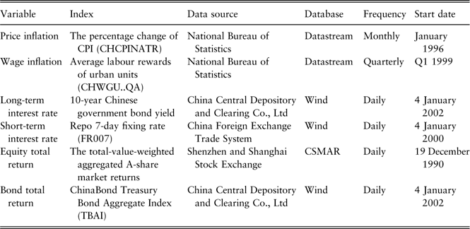
We summarise the data sources for all the variables in Table 1.

Table 1 Data sources.

Price inflation rate. We use the percentage change of consumer price index to reflect the price inflation rate. The OCSB seasonal unit root test resultFootnote ² suggests that there is one seasonal unit root in the CC price inflation rate sequence {p(t)}. Therefore, the seasonal non-stationarity should be removed by taking the seasonal difference Δ₄p(t). Both the original and seasonally differenced time series plots are displayed in Figure 1.

Figure 1 Price inflation rate.

Wage inflation rate. The cumulative average wage of employed staff and workers in urban units without seasonal adjustment is published by the National Bureau of Statistics. The index reflecting the level of wage income is for staff and workers in enterprises, institutions and government agencies. For the quarterly data, the observations refer to the cumulative average wage at the end of each period. Consequently, we need to remove the aggregate effect before using it. Suppose the actual average wage of employed people in time period t is denoted by n(t) and the cumulative average wage to time period t is denoted by m(t) then the actual average wage of employed people can be derived as follows

$$n(t)=\left( {\matrix{ \!\!\!\!\!\!\!\!\!\!\!\!\!\!\!\!\!\!\!\!\!\!\!\!\!\!\!\!\!\!\!\!\!{m(t),\;{\rm if}\,t\,{\rm is}\,{\rm quarter}\,1} \cr {m(t){\minus}m(t{\minus}1),\;{\rm if}\,t\,{\rm is}\,{\rm not}\,{\rm quarter}\,1} \cr } } \right.$$

The effective wage inflation rate $\bar{w}(t)$ for time period t is $\bar{w}(t)=100{\times}\left( {{{n(t)} \over {n(t{\minus}1)}}{\minus}1} \right)$ and the CC rate is $$w(t)=\ln (1{\plus}\bar{w}(t)/100)$$ . We plot the CC wage inflation rate in the first graph in Figure 2. The strong seasonality within the quarterly wage inflation rate sequence is owing to the fact that rewards in the last quarter of each year are much higher than other quarters, which is a common phenomenon in Chinese institutions and enterprises and is called end-of-year rewards. By conducting the seasonal unit root test, we find that there is a seasonal unit root in the CC wage inflation rate sequence {w(t)}. By seasonal differencing of the data, we obtain stationary time series {Δ₄w(t)}, which is shown in the second graph of Figure 2.

Figure 2 Wage inflation rate.

Long-term interest rate. Ten-year Chinese government bond yield is used to represent the long-term interest rate. Both ADF and PP unit root tests of the CC long-term interest rate {l(t)} suggest one unit root. Hence, we difference the data to obtain the stationary sequence {Δl(t)}. Both the original and differenced time series plots are shown in Figure 3.

Figure 3 Long-term interest rate.

Short-term interest rate. Repo 7-day fixing rate is applied as the Chinese short-term interest rate, which is to be used for cash investment. Besides the Repo 7-day fixing rate, there are other candidate proxies for this variable, such as China interbank offered rate (Chibor), Shanghai interbank offered rate (Shibor) and 1-year deposit rate. We choose to use the Repo 7-day fixing rate for several reasons. First, the Thomson Reuters China Pension Fund Index, which is used for enterprise annuities (EA)Footnote ³, changed their short-term interest rate index from the 1-year deposit rate to Repo 7-day fixing rate for cash investment in 2011. Second, another well-accepted index Shibor has a very similar data pattern with the Repo 7-day fixing rate; however, its data starts from 2006, which gives only 6 years of history. In addition, Wang (Reference Wang2012) shows that Repo 7-day fixing rate is the best benchmark short-term interest rate for China based on an empirical study of several possible indices.

Both the ADF and PP unit root tests suggest a unit root in the CC short-term interest rate {s(t)}. So we calculate the difference in the data to obtain stationary time series {Δs(t)}. Both the original and differenced time series plots are displayed in Figure 4. The unusually high volatility that can be observed since December 2010 is owing to reasons such as the slowdown of external liquidity inflow and declined deposit growth rate (see Pan & Cao, Reference Pan and Cao2012).

Figure 4 Short-term interest rate.

Equity total return. The total-value-weighted aggregated market returns are obtained from CSMAR database, which is published via regular and interim announcements from companies listed in Shenzhen and Shanghai A Share Stock Markets (for domestic investors only). Another candidate proxy is China Security Index 300, which includes both the price index and total return index. However, the total return index is only available from 2006. So we have to use the total-value-weighted aggregated market returns from CSMAR to obtain more observations. The CC equity total return sequence is derived from the monthly sequence. The time series plot of {e(t)} is shown in Figure 5. There is a trough in 2008 that is because of the global financial crisis.

Figure 5 Equity total return.

Bond total return. In general, pension funds or insurance companies could invest in bonds with various durations and credit ratings. So we model bond total return as an approximation to all the investment possibilities. ChinaBond treasury bond aggregate index is used as the proxy for Chinese bond total return. This index includes treasury bonds, financial bonds and corporate bonds listed on Shanghai Stock Exchange, Shenzhen Stock Exchange and the interbank market. The terms to maturity are above 1 year. The index is calculated by assuming coupons are reinvested into the bond index. The CC bond total return {b(t)} is stationary and shown in Figure 6. The peak in 2008 is also because of the global financial crisis as investors moved from the equity market to the bond market.

Figure 6 Bond total return.

All variables are summarised in Table 2. Unless otherwise specified, all values of these variables are expressed as percentages throughout this paper. We always use CC rates of return for modelling purposes, except for the long-term interest rate model in the Wilkie-type (price-inflation-driving) cascade system in section 3.3.2, where we model the effective long-term interest rate to be consistent with the original Wilkie model.

Table 2 Variables.

3. Models

In this section, we will investigate three modelling structures: univariate models, VAR and cascade systems. Greek letters, such as μ, α, β, are used to denote coefficients in the models. $\epsilon (t)$ is to denote the error term. In addition, subscripts of the notations are used to distinguish the coefficients for different variables, for example, μ _p and α _p will appear in the model for price inflation rate p(t); 1%, 5% and 10% significance levels are denoted by ***, ** and * respectively, for parameters estimated and relevant statistics.

3.1. Univariate models

Univariate models do not take interrelationships among variables into consideration and exclude the effects of exogenous variables. Box & Jenkins (Reference Box and Jenkins1976) methodology entails three steps to build univariate ARIMA models: model identification, model estimation and model diagnostic checking. Their aim is to provide a technique that leads to parsimonious models. In this paper, the modelling process is described using similar processes with references from modern econometrics (see Hamilton, Reference Hamilton1994; Enders, Reference Enders2010). To begin, we define the ARIMA model and other related models as follows.

Definition 1. Suppose {y(t)} is a stochastic process with the following formulation

$$y(t)=\alpha _{0} {\plus}\mathop{\sum}\limits_{i=1}^p \alpha _{i} y(t{\minus}i){\plus}\epsilon (t){\plus}\mathop{\sum}\limits_{i=1}^q \beta _{i} \epsilon (t{\minus}i)$$

where $\{ \epsilon (t)\} $ is a white-noise process. If all the characteristic rootsFootnote ⁴ of equation (1) lie outside the unit circle, {y(t)} is called an autoregressive moving-average process (ARMA) (p,q). If one or more characteristic roots of equation (1) is greater than or equal to unity, the {y(t)} is called an integrated process and equation (1) is called an ARIMA. If the homogeneous partFootnote ⁵ of equation (1) has d unit roots, then the process {y(t)} is integrated of order d, denoted by I(d). And the d ^th difference of {y(t)}, denoted by {Δ^dy(t)}, is stationary. The ARIMA model for y(t) is denoted by ARIMA (p,d,q), with the interpretation that the d ^th difference of {y(t)} is a stationary ARMA (p,q) process.

Model identification. This is the first stage in the modelling process. The autocorrelation function (ACF) and the partial autocorrelation function (PACF) are used to identify lags of variables that should be incorporated. Generally speaking, it is convenient to use the PACF to identify the lag of the autoregressive component and use ACF to identify the lag of the moving-average component. However, it is still complicated to identify the model structures definitely. Hence, to determine the best p and q in equation (1), we estimate models with different lags and then use Akaike information criterion (AIC) and Bayesian information criterion (BIC) goodness-of-fit measures to select the model with the best fit. There are a number of different ways to report the AIC and BIC. In this paper we use the following definitions

$$\eqalignno{ {AIC}\ & {={\minus}2ln(L)/T{\plus}2n/T,} \hfill \cr {BIC}\ & {={\minus}2ln(L)/T{\plus}ln(T){\times}n/T} \hfill \cr } $$

where L is the maximised value of the log of the likelihood function, n the number of parameters estimated and T the number of observations used for model fitting. Both AIC and BIC have penalties on the number of parameters, and BIC selects more parsimonious model. The smaller is the value of AIC or BIC, the better is the model fitted.

Model estimation. In this paper, the ordinary least squares estimation method is applied. The Newey–West heteroskedasticity and autocorrelation consistent estimation is used to generate robust standard errors.

For GARCHFootnote ⁶ models, maximum likelihood estimation techniques are applied for model estimation. Robust standard errors are estimated using the Bollerslev & Wooldridge (Reference Bollerslev and Wooldridge1992) method.

For the model fitting, we always use the whole period of the data history from the second quarter of 2002 to the fourth quarter of 2012.

Model checking. We check the model from different perspectives, such as the normality and correlations of residuals, goodness-of-fit measures, significance of parameters and out-of-sample validation.

In this paper, we assume the error terms of stochastic models follow Gaussian white-noise processes. The normality of residuals is tested using Jarque–Bera (JB) statistic. The test statistic is defined as

$$JB={n \over 6}{\times}\left( {S^{2} {\plus}{1 \over 4}(K{\minus}3)^{2} } \right)$$

where n is the number of observations, S the sample skewness and K the sample kurtosis. If the data follows a normal distribution, the JB statistic asymptotically follows a χ ² distribution with 2 degrees of freedom.

Independence of the residuals is tested using the ACF and PACF of residuals. Conditional heteroscedasticity of residuals is tested using the ACF and PACF of squared residuals. The Ljung–Box Q-statistic is the test statistic for autocorrelations, which is an asymptotically χ ² distribution with degrees of freedom equal to the number of autocorrelations. Q-statistics at lag one are denoted by AC1(Res) and AC1(Res ²) for the autocorrelations of residuals and squared residuals, respectively.

Goodness-of-fit is tested using AIC and BIC measures, which are discussed above. Significance of parameters is tested using t-tests and F-tests; and t-tests are used to test the significance of a single parameter, while F-tests are to test the significance of a group of parameters. Both of the two tests are used to identify the insignificant parameters and streamline the model. In this paper, we only provide the results of t-tests for parameters in the model that we derive for each variable.

Out-of-sample validations are conducted to evaluate the forecasting performance. Suppose there are n+h observations in total. We use the first n observations for estimation and then use the estimated parameters to generate a one-step-ahead forecast. We then use the generated one-step-ahead forecast observation and estimated coefficients to obtain a second one-step-ahead forecast. Similar methods are applied to generate h one-step-ahead forecasts. The forecast sample is from n+1 to n+h. And we denote the the actual and forecasted values in period t (t ranges from n+1 to n+h) as y(t) and $$\hat{y}(t)$$ . The root mean square forecast error (RMSFE) is defined as follows

$$RMSFE=\sqrt {{1 \over h}\mathop{\sum}\limits_{t=n{\plus}1}^{n{\plus}h} (\hat{y}(t){\minus}y(t))^{2} } $$

RMSFE is used for model selection, and we should select the model with the smallest RMSFE. In this paper, to conduct an out-of-sample validation, the estimation sample is from the second quarter of 2002 to the fourth quarter of 2010; and the forecast sample is from the first quarter of 2011 to the fourth quarter of 2012. However, for model fitting, we always use the whole data period from the second quarter of 2002 to the fourth quarter of 2012. All values of RMSFE are based on CC non-differenced variables.

3.1.1. Price inflation rate

The seasonal differenced price inflation rate Δ₄p(t) is modelled by an AR(1) process:

$$\Delta _{4} p(t)=\alpha _{p} \Delta _{4} p(t{\minus}1){\plus}\epsilon _{p} (t)$$

To interpret the model, the differenced price inflation rate in time period t is proportion to the differenced term in the previous period t−1. The estimation results are shown in Table 3. As discussed above, 1%, 5% and 10% significance levels are denoted by ***, ** and * respectively, for parameters estimated and relevant statistics. So if there is no asterisk with the test statistics, it means the statistics can be regarded as insignificant. For example, in Table 3, the estimated value of α _p is significant at 5% level, AC1(Res), AC1(Res ²) and JB statistic are insignificant based on all three levels. The robust standard error of the parameter estimation is provided in brackets. The results indicate that residuals are normally distributed and exhibit no autocorrelations.

Table 3 Estimations for price inflation rate.

**significant at the 5% level.

AIC, Akaike information criterion; BIC, Bayesian information criterion; RMSFE, root mean square forecast error.

3.1.2. Wage inflation rate

The seasonal differenced wage inflation rate Δ₄w(t) is modelled as a white-noise process:

$$\Delta _{4} w(t)=\epsilon _{w} (t)$$

There is no parameter estimation in this model. The diagnostic checking of results is shown in Table 4. Residuals are normally distributed with no particularly significant autocorrelations.

Table 4 Estimations for wage inflation rate.

*significant at the 10% level.

AIC, Akaike information criterion; BIC, Bayesian information criterion; RMSFE, root mean square forecast error.

3.1.3. Long-term interest rate

The first differenced long-term interest rate Δl(t) is modelled as a white-noise process:

$$\Delta l(t)=\epsilon _{l} (t)$$

Diagnostic checking of the results is shown in Table 5. Residuals are normally distributed. There is no evidence of significant autocorrelations in residuals.

Table 5 Estimations for long-term interest rate.

AIC, Akaike information criterion; BIC, Bayesian information criterion; RMSFE, root mean square forecast error.

3.1.4. Short-term interest rate

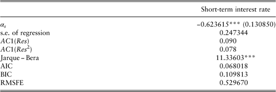
The differenced short-term interest rate Δs(t) is modelled as an AR(1) process:

$$\Delta s(t)=\alpha _{s} \Delta s(t{\minus}1){\plus}\epsilon _{s} (t)$$

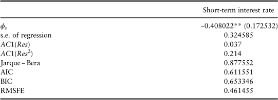
To interpret the model, the differenced quarterly short-term interest rate in time period t is a proportion of the differenced term in the previous period t−1. Estimated parameters are in Table 6. The hypothesis of normally distributed residuals is rejected because of the high volatility from December 2010. A regime-switching model may be appropriate in this case but has not been tested owing to the limitation of data. We have also tried the GARCH framework; however, it does not provide a better model based on AIC, BIC and RMSFE measures. There is no evidence of autocorrelations in residuals.

Table 6 Estimations for short-term interest rate.

***significant at the 1% level.

AIC, Akaike information criterion; BIC, Bayesian information criterion; RMSFE, root mean square forecast error.

3.1.5. Equity total return

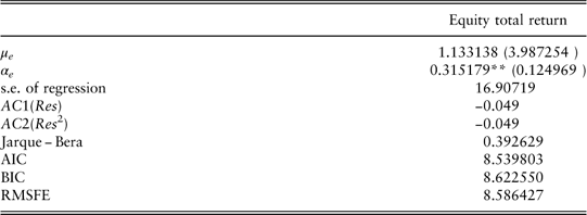
The equity total return e(t) follows an AR(1) process:

$$\eqalignno{ {e(t)} \hfill \,& {\,=\,\mu _{e} {\plus}x_{e} (t)} \hfill \cr {x_{e} (t)} \hfill \,& {\,=\,\alpha _{e} x_{e} (t{\minus}1){\plus}\epsilon _{e} (t)} (6)} $$

where μ _e is the long-term mean. The estimation results are shown in Table 7. The residuals are normality distributed and are not autocorrelated.

Table 7 Estimations for equity total return.

**significant at the 5% level.

AIC, Akaike information criterion; BIC, Bayesian information criterion; RMSFE, root mean square forecast error.

3.1.6. Bond total return

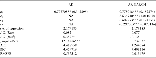
A white-noise process is assumed for the bond total return b(t):

$$b(t)=\mu _{b} {\plus}\epsilon _{b} (t)$$

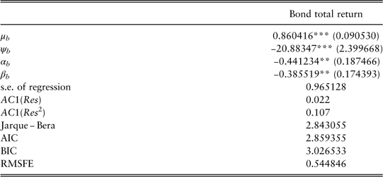
μ _b refers to the expected quarterly bond total return in the long run. The estimated parameters and diagnostic checking of results are shown in Table 8. Residuals are not normally distributed owing to the peak in year 2008. Although there is no autocorrelations of residuals, the squared residuals are autocorrelated and indicate a GARCH (1, 1) structure to capture the conditional heteroskedasticity. Following Bollerslev (Reference Bollerslev1986), a GARCH (p,q) process is defined as follows

$$\eqalignno{ {\epsilon (t)} \hfill \,& {=\nu (t)\sqrt {h(t)} } \hfill \cr {h(t)} \hfill \,& {=c_{0} {\plus}\mathop{\sum}\limits_{i=1}^q c_{i} \epsilon ^{2} (t{\minus}i){\plus}\mathop{\sum}\limits_{i=1}^p d_{i} h(t{\minus}i)} (8)} $$

where {ν(t)} is a white-noise process with variance $\sigma _{\nu }^{2} =1$ ; $\epsilon (t)$ and ν(t) are independent; h(t) can be derived to be the conditional variance of $\epsilon (t)$ ; c _i (i=0,1,...,q) and d _i (i=1,2,...,p) are coefficients.

Table 8 Estimations for bond total return.

**significant at the 5% level; ***significant at the 1% level.

AR-GARCH, autoregressive generalised autoregressive conditionally heteroscedastic; AIC, Akaike information criterion; BIC, Bayesian information criterion; RMSFE, root mean square forecast error.

Compared with the AR model, the normality of residuals is satisfied in the AR-GARCH model. However, the AR model has better forecasting performance based on the out-of-sample validation. So we choose to use the AR model for further comparisons with other models.

3.1.7. Summary

We summarise the model structures and model estimations in Table 9 and Table 10, respectively.

Table 9 Univariate model structures.

Table 10 Univariate model estimations.

**significant at the 5% level; ***significant at the 1% level.

Univariate model checking is presented in Table 11. Given that the first-order autocorrelation of residuals from all the models are insignificant, parameters are significant (except for models of equity total return and bond total return, which are required to be kept to ensure a non-zero mean return), the model checking statistics summarised here only include residual normality checking statistics JB, model selection measures AIC and BIC, and out-of-sample validation measure RMSFE.

Table 11 Univariate model checking.

***significant at the 1% level.

AIC, Akaike information criterion; BIC, Bayesian information criterion; RMSFE, root mean square forecast error.

3.1.8. Correlations of residuals

Table 12 shows the contemporaneous correlations of residuals in the univariate models. The results indicate that there are significant correlations among residuals, which means that the univariate models ignore some correlation patterns among variables. For example, the bond total return and long-term interest rate have very significant correlation, which is reasonable as the long-term interest rate (10-year government bond yield) affects the bond prices and hence affects the bond total return. Under the circumstances, multivariate models should also be investigated to take the correlations among variables into consideration.

Table 12 Univariate model: residual correlations.

Values in bold indicate significant correlations.

*significant at the 10% level; **significant at the 5% level; ***significant at the 1% level.

3.2. VAR

VAR models treat each variable symmetrically. We consider the stationary variables from Table 2 for modelling purposes. Information criterion are employed widely to determine the appropriate lag order of VAR (see Lütkepohl, Reference Lütkepohl1991). In this paper, LR (sequential modified LR test statistic), final prediction error, AIC, BIC and Hannan–Quinn information criterion) are applied for lag-order selections and the lag-order selection results indicate that we should choose the first-order VAR for modelling purposes.

The first-order VAR structure is as follows

$$\eqalignno{ \left[ {\matrix{ {\Delta _{4} p(t)} \cr {\Delta _{4} w(t)} \cr {\Delta l(t)} \cr {\Delta s(t)} \cr {e(t)} \cr {b(t)} \cr } } \right]=\left[ {\matrix{ {a_{{10}} } \cr {a_{{20}} } \cr {a_{{30}} } \cr {a_{{40}} } \cr {a_{{50}} } \cr {a_{{60}} } \cr } } \right]{\plus} & \left[ {\matrix{ {a_{{11}} } & {a_{{12}} } & {a_{{13}} } & {a_{{14}} } & {a_{{15}} } & {a_{{16}} } \cr {a_{{21}} } & {a_{{22}} } & {a_{{23}} } & {a_{{24}} } & {a_{{25}} } & {a_{{26}} } \cr {a_{{31}} } & {a_{{32}} } & {a_{{33}} } & {a_{{34}} } & {a_{{35}} } & {a_{{36}} } \cr {a_{{41}} } & {a_{{42}} } & {a_{{43}} } & {a_{{44}} } & {a_{{45}} } & {a_{{46}} } \cr {a_{{51}} } & {a_{{52}} } & {a_{{53}} } & {a_{{54}} } & {a_{{55}} } & {a_{{56}} } \cr {a_{{61}} } & {a_{{62}} } & {a_{{63}} } & {a_{{64}} } & {a_{{65}} } & {a_{{66}} } \cr } } \right]\left[ {\matrix{ {\Delta _{4} p(t{\minus}1)} \cr {\Delta _{4} w(t{\minus}1)} \cr {\Delta l(t{\minus}1)} \cr {\Delta s(t{\minus}1)} \cr {e(t{\minus}1)} \cr {b(t{\minus}1)} \cr } } \right] \cr {\plus}\left[ {\matrix{ {\eta _{1} (t)} \cr {\eta _{2} (t)} \cr {\eta _{3} (t)} \cr {\eta _{4} (t)} \cr {\eta _{5} (t)} \cr {\eta _{6} (t)} \cr } } \right] $$

where a _ij (i, j=1,2,...,6) are the coefficients and η(t) the error term for each equation. It is crucial to note that the error terms are correlated with each other.

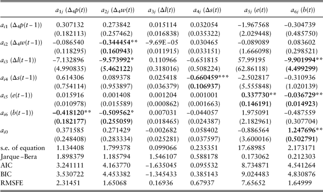
The estimation results are shown in Table 13, where robust standard errors of estimations are presented within brackets. The model checking procedures are similar with those in univariate modelling. The results show that there are many insignificant parameters. According to Enders (Reference Enders2010), unrestricted VARs are overparameterised, and may not be reliable for forecasting. In order to obtain a more parsimonious model for forecasting purposes, we remove the insignificant coefficients and obtain a near-VAR model, which is reestimated using seemingly unrelated regressions (SUR) (see Enders, Reference Enders2010). However, based on the model selection criterion, the near-VAR model does not perform significantly better than the VAR model, and is hence not pursued further. So, in order to obtain a parsimonious model with better performance, we move on to explore the cascade structure in section 3.3.

Table 13 VAR model estimations.

Values in bold indicate significant parameters.

*significant at the 10% level; **significant at the 5% level; ***significant at the 1% level.

VAR, vector autoregression; AIC, Akaike information criterion; BIC, Bayesian information criterion; RMSFE, root mean square forecast error.

3.3. Cascade systems

Although the VAR structure considers correlations among variables, it has some drawbacks for forecasting, such as many insignificant estimated parameters and difficulty in capturing all the patterns within variables. The aim of this subsection is to build a cascade system to circumvent these problems. The definition of a cascade system is as follows.

Definition 2. Suppose there are n stationary time series {x ₁(t)},{x ₂(t)},…,{x _n(t)}. We assume one of the variables x ₁(t) is the driving force of the others x ₂(t),x ₃(t),…x _n(t). The {x ₁(t)} sequence is modelled as a univariate ARMA process. The other variables are modelled with inputs as x ₁(t) and/or other variables using TFM (see Definition 3). The whole structure is called a cascade system.

We introduce the definition of a TFM following Enders (Reference Enders2010).

Definition 3. The TFM is defined as the following equation

$$y(t)=a_{0} {\plus}A(L)y(t{\minus}1){\plus}C(L)x(t){\plus}B(L)\epsilon (t)$$

where y(t) is the variable to be modelled; x(t) is another variable in the cascade system; $$\{ \epsilon (t)\} $$ is a white-noise process; A(L), B(L) and C(L) are polynomials in the lag operator L. C(L) is called the transfer function. In other words, the time path of {y(t)} is affected by the time path of {x(t)} without feedback.

Wilkie (Reference Wilkie1986, Reference Wilkie1995) first uses the cascade structure to project economic variables of the United Kingdom. In his papers, the price inflation rate is assumed to be the driving force of all the other variables. The model structures are derived by examining the time series plots and applying some economic relationships, such as the Fisher (Reference Fisher1930) effect. Dickson (Reference Dickson2001) reports that there have been actuaries in other countries, who have claimed that the Wilkie model is inappropriate to their local conditions, and who have to produce their own stochastic economic models. Therefore, it is significant to derive a generalised methodology, which could be used to build a cascade system for many other countries. In this paper, we use Granger causality tests to identify the driving force. A generalised Wilkie structure is presented based on data rather than economic theories.

Suppose there are several stationary time series to be modelled and two of them are denoted as {y _t} and {z _t}. A p ^th order VAR model for {x(t)} and {y(t)} using lag operator L is

$$\left[ {\matrix{ {x(t)} \cr {y(t)} \cr } } \right]=\left[ {\matrix{ {A_{{10}} } \cr {A_{{20}} } \cr } } \right]{\plus}\left[ {\matrix{ {A_{{11}} (L)} & {A_{{12}} (L)} \cr {A_{{21}} (L)} & {A_{{22}} (L)} \cr } } \right]\left[ {\matrix{ {x_{1} (t{\minus}1)} \cr {y_{1} (t{\minus}1)} \cr } } \right]{\plus}\left[ {\matrix{ {\eta _{x} (t)} \cr {\eta _{y} (t)} \cr } } \right]$$

where η _x(t) and η _y(t) are the error terms; A _i0 (i=1,2) are the parameters of intercept terms; and $a_{{ij}}^{k} (k=1,2,\,\,\ldots\,p,)$ are the coefficients of A _ij(L). The test of Granger causality is used to investigate whether the lags of one variable enter into the equation of the other variable. With reference to Enders (Reference Enders2010), we define the Granger causality for a bivariate model as follows.

Definition 4. In equation (11), {x(t)} does not Granger cause {y(t)} if and only if all the coefficients in A ₂₁(L) are equal to 0, which indicates that the current and past values of {x(t)} do not improve the forecasting performance of {y(t)}. If {x(t)} Granger causes {y(t)}, we denote x(t) → y(t).

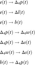
In applications, a large lag order is suggested to be employed for Granger causality testing so that the autocorrelation patterns within the series are completely incorporated. Hence, we always choose the largest possible lag order for each pair of Granger causality test in this research. The variable, which is not Granger caused by other variables, should be regarded as the driving force. Based on the Chinese data, stationary variables are considered and the significant pairwise Granger causality relationships are listed below

$$\eqalignno{ & e(t)\to\Delta _{4} p(t) \cr & e(t)\to\Delta l(t) \cr & e(t)\to\\b(t) \cr & \Delta _{4} p(t)\to\Delta _{4} w(t) \cr & \Delta _{4} p(t)\to\Delta s(t) \cr & \Delta _{4} w(t)\to\Delta s(t) \cr & b(t)\to\Delta _{4} p(t) $$

It is crucial to note that the Granger causality does not indicate real causal relationships. For example e(t) → b(t) should be interpreted in this way: given that b(t) is modelled with its own lagged values, the past and current values of e(t) still help to forecast the future values of b(t). In this case, variables in the right-hand side of the arrow sign should not be treated as the driving force. Consequently, we derive that the equity total return is the driving force. A univariate ARMA model should be specified for the equity total return. It is important to note that the Granger causality tests are only used to identify the driving force, and explicit model structures for other variables are investigated one by one using autoregressive distributed lag (ADL) modelling techniques as introduced below. Pairwise Granger causality testing results shown in equation (12) may not be the best models according to our model selection criterion. So for each response variable, we test all the other variables with various lags as predictors under the ADL framework. In addition, we also test models suggested in other papers, such as Wilkie (Reference Wilkie1995). Then, all the tested models are compared according to our model selection criterion and the best structure for each variable is derived.

To identify the TFM structure for variables that are not the driving force, we transform equation (10) to an ADL model in the following form

$$y(t)=a_{0} {\plus}\mathop{\sum}\limits_{i=1}^p {a_{i} y(t{\minus}i){\plus}\mathop{\sum}\limits_{i=0}^q {c_{i} x(t{\minus}i){\plus}\epsilon (t)} } $$

To estimate an ADL model, we have to begin by using the largest values of p and q. After that F-tests and t-tests are used to identify insignificant parameters and streamline the model. At the same time, AIC and BIC goodness-of-fit measures are applied to select the model with the best fit. Diagnostic checking of results is performed in the same way as for univariate modelling.

3.3.1. The equity-driving system

The equity-driving cascade system is built under the assumption that the equity total return is the driving force, which is similar with the driving force derived based on the South African data in Thomson (Reference Thomson1996). The equity-driving cascade structure is illustrated in Figure 7. The price inflation and long-term interest rate are affected directly by the equity total return. The wage inflation is linked with the price inflation. And the short-term interest rate and bond total return are affected by the long-term interest rate.

Figure 7 The structure of the equity-driving cascade system.

Equity total return. This is the driving force in the cascade modelling structure, whose framework should be the same as the univariate model, that is an AR(1) process:

$$\eqalignno{ {e(t)} \hfill \,& {=\mu _{e} {\plus}x_{e} (t)} \hfill \cr {x_{e} (t)} \hfill \,& {=\alpha _{e} x_{e} (t{\minus}1){\plus}\epsilon _{e} (t)} (14)} $$

The estimations and model checking of results are in Table 7. The positive α _e means an element of short-term momentum.

Price inflation rate. The seasonal differenced price inflation rate is derived to be linked with two periods lagged equity total return:

$$\Delta _{4} p(t)=\psi _{p} (e(t{\minus}2){\minus}\mu _{e} ){\plus}\epsilon _{p} (t)$$

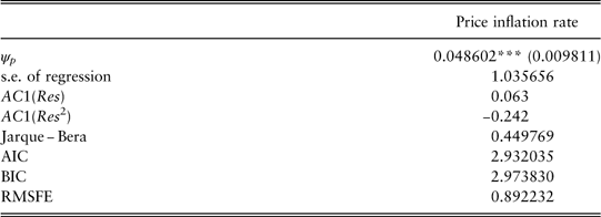
Under the ADL framework, we have tried different models with different lag orders, however, this model turns out to be the best one according to our model selection criterion. The seasonal differenced price inflation rate is modelled as a proportion of the difference between the two periods lagged equity total return and its long-term mean. This model indicates that if the equity total return moves higher (lower) than its long-term mean, then the price inflation rate also tends to increase (decrease) two periods later compared with the same period last year. This is analogous to good (poor) economic performance (as measured by equity returns) leading to future increases (decreases) in general prices. The estimations and diagnostic checking of results are presented in Table 14. The Jarque–Bera normality test indicates that residuals are normally distributed. Autocorrelations of residuals are insignificant and there is no evidence of conditional heteroscedasticity.

Table 14 Estimations for price inflation rate.

***significant at the 1% level.

AIC, Akaike information criterion; BIC, Bayesian information criterion; RMSFE, root mean square forecast error.

Wage inflation rate. The seasonal differenced wage inflation rate Δ₄w(t) is linked with the seasonal differenced price inflation rate Δ₄p(t), with the assumption that the level of the price inflation rate affects the time pace of the wage inflation rate. The model is as follows

$$\matrix{ {\Delta _{4} w(t)=\psi _{w} \Delta _{4} p(t){\plus}x_{w} (t)} \cr \quad \ {x_{w} (t)=\alpha _{w} x_{w} (t{\minus}1){\plus}\epsilon _{w} (t)} \cr } $$

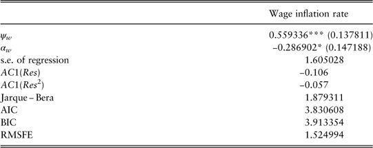
To interpret the model, the seasonal differenced wage inflation rate Δ₄w(t) is modelled by a proportion ψ _w of the contemporaneous seasonal differenced price inflation rate Δ₄p(t) and an AR(1) process without the mean term. This is an intuitive result given that we expect prices and wages to be correlated. The estimated coefficients and diagnostic checking of results are presented in Table 15. It is evident that the residuals are normally distributed, and there is no evidence of autocorrelations in residuals.

Table 15 Estimations for wage inflation rate.

*significant at the 10% level; ***significant at the 1% level.

VAR, vector autoregression; AIC, Akaike information criterion; BIC, Bayesian information criterion; RMSFE, root mean square forecast error.

Long-term interest rate. The first differenced long-term interest rate is derived to be driven by the equity total return and is modelled as a proportion of the difference between the contemporaneous equity total return and its long-term mean. The model is

$$\Delta l(t)=\psi _{l} (e(t){\minus}\mu _{e} ){\plus}\epsilon _{l} (t)$$

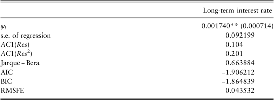
It means that if the equity total return moves higher (lower) than its long-term mean, the contemporaneous long-term interest rate also tends to increase (decrease) compared with last period. This is analogous to investors factoring in an increase (decrease) in general interest rates upon good (poor) economic performance (as measured by equity returns). This structure is also consistent with the macroeconomic policy of the Chinese government: when the country’s equity market is at risk of overheating, the government would increase the benchmark 1-year deposit and lending interest rates to cool down the economy, which would further affect the long-term interest rates (see Li, Reference Li2007). This model is similar with the model for the price inflation rate in equation (15), while the price inflation is affected by the lagged equity total return and the long-term interest rate is affected by the contemporaneous equity total return. The estimations and diagnostic checking of results are shown in Table 16. We find that the residuals can be regarded as normally distributed, and there is no evidence of autocorrelations in residuals.

Table 16 Estimations for long-term interest rate.

**significant at the 5% level.

AIC, Akaike information criterion; BIC, Bayesian information criterion; RMSFE, root mean square forecast error.

Short-term interest rate. As discussed before, we test various structures including a modified short-term interest rate model in Wilkie (Reference Wilkie1995). By applying the model selection criterion, we find that the modified Wilkie model is the best. To build the model, we first compute the sequence {ln(l(t))−ln(s(t))}, which is non-stationary based on ACF and PP unit root tests. So we first difference the sequence and then model it as an AR(1) process in the following form

$$\matrix{ {\Delta [{\rm ln}(l(t)){\minus}{\rm ln}(s(t))]=x_{s} (t)} \cr {x_{s} (t)=\phi _{s} x_{s} (t{\minus}1){\plus}\epsilon _{s} (t)} \cr } $$

The estimated coefficients and diagnostic checking of results are presented in Table 17. There is nothing unusual in the residual analysis and no conditional heteroskedasticity is observed.

Table 17 Estimations for short-term interest rate.

**significant at the 5% level.

AIC, Akaike information criterion; BIC, Bayesian information criterion; RMSFE, root mean square forecast error.

Bond total return. The bond total return is modelled as the contemporaneous effect of the first differenced long-term interest rate plus a second-order autoregressive component:

$$\eqalignno{ {b(t)} \hfill \,& {=\mu _{b} {\plus}\psi _{b} \Delta l(t){\plus}x_{b} (t)} \hfill \cr {x_{b} (t)} \hfill \,& {=\alpha _{b} x_{b} (t{\minus}1){\plus}\beta _{b} x_{b} (t{\minus}2){\plus}\epsilon _{b} (t)} \hfill (19) $$

where μ _b is the long-term mean of bond total return. It is intuitive that bond returns are linked with changes in bond yields and the long-term interest rates end up proxying for bond yields. We have also tested models that have undifferenced or differenced long-term and/or short-term interest rates as explanatory variables, which, however, do not perform better than equation (19), according to our model selection criterion. The residual diagnostic checking of results in Table 18 show that the normality assumption of residuals holds. There is no evidence of autocorrelations in residuals.

Table 18 Estimations for bond total return.

**significant at the 5% level; ***significant at the 1% level.

AIC, Akaike information criterion; BIC, Bayesian information criterion; RMSFE, root mean square forecast error.

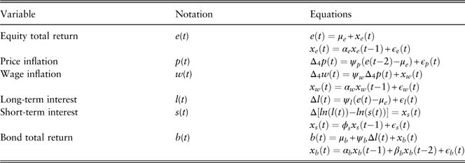
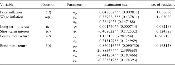
Summary.Table 19 presents the models developed based on quarterly data. The parameter estimations of the models are summarised in Table 20. And the summarised model checking of results are in Table 21. We can observe that the standard error of the residuals and RMSFE for equity total return model is much higher than others. The reason is owing to the much higher volatility of equity total returns as shown in Figure 5.

Table 19 Equity-driving cascade system: model structures.

Table 20 Equity-driving cascade system: model estimations.

*significant at the 10% level; **significant at the 5% level; ***significant at the 1% level.

Table 21 Equity-driving cascade system: model checking.

AIC, Akaike information criterion; BIC, Bayesian information criterion; RMSFE, root mean square forecast error.

Correlations of residuals. The correlations of residuals are helpful to check whether the correlations of variables have been well captured. The results shown in Table 22 indicate that there are no contemporaneous correlations among residuals at the significance level of 5%. We have also tried to model bond total return with both first differenced short-term interest rates and first differenced long-term interest rates. In this case, although the significant correlation at 10% level between bond total return and short-term interest rate disappear, the model performs worse according to our model selection criterion (which prefer a more parsimonious model).

Table 22 Equity-driving cascade system: residual correlations.

Values in bold indicate significant correlations.

*significant at the 10% level.

3.3.2. The price-inflation-driving system

The Wilkie (Reference Wilkie1986, Reference Wilkie1995) model has been widely accepted and discussed in developed countries. Although the driving force variable has been identified as the equity total return for the Chinese data at the beginning of section 3.3, the Wilkie-type structure is still employed for comparison purposes. Some variables used in this paper are different from those in the Wilkie model. For example, the equity total return and bond total return are not considered in the Wilkie structure. Instead, Wilkie models the equity dividend and dividend yield. In this circumstances, the Wilkie-type frameworks are modified where necessary.

The cascade structure of the price-inflation-driving system (Wilkie-type model) is illustrated in Figure 8. It shows that if we assume the price inflation to be the driving force, the equity total return is not related with any other variable. The price inflation model is the same as the univariate model. And the wage inflation, short-term interest rate and bond total return are the same as those in the equity-driving cascade system. Therefore, the model of long-term interest rates is the only one that is different from previous models.

Figure 8 The structure of the price-inflation-driving cascade system.

Long-term interest rate. The Wilkie model for long-term interest rate models the effective rate of return rather than CC rate of return. So here we also use the effective long-term interest rate $$\bar{l}(t)$$ for modelling purposes. We introduce a modified version of the long-term interest rate model in Wilkie (Reference Wilkie1995):

$$\eqalignno{ {\bar{l}(t)} \hfill \,& {=\gamma _{l} c_{l} (t){\plus}\rho _{l} exp(x_{l} (t))} \hfill \cr {c_{l} (t)} \hfill \,& {=\psi _{l} p(t){\plus}(1{\minus}\psi _{l} )c_{l} (t{\minus}1)} \hfill \cr {x_{l} (t)} \hfill \,& {=\alpha _{l} x_{l} (t{\minus}1){\plus}\beta _{l} {\varepsilon}_{e} (t){\plus}\epsilon _{l} (t)} \hfill (20)$$

where the effective long-term interest rate $\bar{l}(t)$ is linked with the price inflation rate. In equation (20), c _l(t) is an exponentially weighted moving average of the price inflation, which represents the unit gain from the price inflation. x _l(t) is a first-order autoregressive process and $\epsilon _{e} (t)$ the error term from the equity total return modelFootnote ⁷. With γ _l=1, the model fully takes the “Fisher effect'” into consideration. So for simplicity, γ _l is set to be 1. However, when applying the framework to the Chinese data, we find that $\bar{l}(t){\minus}c_{l} (t)$ contains many negative values owing to the high inflation rate, which is not suitable for further modelling. In this case, we modify equation (20) and derive the following form

$$\eqalignno{ {\bar{l}(t)} \hfill \,& {=c_{l} (t){\plus}x_{l} (t)} \hfill \cr {c_{l} (t)} \hfill \,& {=\psi _{l} p_{l} (t){\plus}(1{\minus}\psi _{l} )c_{l} (t{\minus}1)} \hfill \cr {\Delta _{4} x_{l} (t)} \hfill \,& {=\alpha _{l} \Delta _{4} x_{l} (t{\minus}1){\plus}\epsilon _{l} (t)} (21)} $$

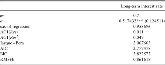
where the long-term interest rate consists of the price inflation effect c _l(t) and the real interest component x _l(t). We set ψ _l to be 0.7, so that the mean of the real term is around 0.2%, which is the expected real long-term interest rate over the entire estimation period. The seasonal unit root test indicates that x _l(t) contains one seasonal unit root. So we remove the seasonal unit root and model Δ₄x _l(t) as a first-order autoregressive process. We also find that the error term of equity total return has no effect on the long-term interest rate, so $\epsilon _{e} (t)$ is excluded in equation (21).

The estimations for the long-term interest model are shown in Table 23. For the residuals, there is no evidence of autocorrelation and the assumption of normality holds.

Table 23 Estimations for long-term interest rate.

***significant at the 1% level.

AIC, Akaike information criterion; BIC, Bayesian information criterion; RMSFE, root mean square forecast error.

4. Model selection

In this section, JB statistic, AIC, BIC and RMSFE are used for model selection among univariate models, VAR, equity-driving and price-inflation-driving cascade systems for each variable. We indicate the significance levels of JB statistic of residuals by ***, ** and * and insignificant JB values mean that the normality assumptions hold. Values of AIC, BIC and RMSFE in bold are the best according to the selection criteria. For the long-term interest rate model in the price-inflation-driving cascade system and the short-term interest rate model in the equity-driving cascade system, the values of AIC and BIC are not suitable for comparisons with other models, as the sequences for modelling are not the same. So “NA” will be used for the values of AIC and BIC for those models in the model selection tables.

∙ Price inflation rate (Table 24).

Table 24 Model selection: price inflation rate.

Values of AIC, BIC and RMSFE in bold are the best according to the model selection criteria.

VAR, vector autoregression; AIC, Akaike information criterion; BIC, Bayesian information criterion; RMSFE, root mean square forecast error.

∙ Wage inflation rate (Table 25).

Table 25 Model selection: wage inflation rate.

Values of AIC, BIC and RMSFE in bold are the best according to the model selection criteria.

VAR, vector autoregression; AIC, Akaike information criterion; BIC, Bayesian information criterion; RMSFE, root mean square forecast error.

∙ Long-term interest rate (Table 26).

Table 26 Model selection: long-term interest rate.

Values of AIC, BIC and RMSFE in bold are the best according to the model selection criteria.

VAR, vector autoregression; AIC, Akaike information criterion; BIC, Bayesian information criterion; RMSFE, root mean square forecast error.

∙ Short-term interest rate (Table 27).

Table 27 Model selection: short-term interest rate.

Values of AIC, BIC and RMSFE in bold are the best according to the model selection criteria.

***significant at the 1% level.

VAR, vector autoregression; AIC, Akaike information criterion; BIC, Bayesian information criterion; RMSFE, root mean square forecast error.

∙ Equity total return (Table 28).

Table 28 Model selection: equity total return.

Values of AIC, BIC and RMSFE in bold are the best according to the model selection criteria.

VAR, vector autoregression; AIC, Akaike information criterion; BIC, Bayesian information criterion; RMSFE, root mean square forecast error.

∙ Bond total return (Table 29).

Table 29 Model selection: bond total return.

Values of AIC, BIC and RMSFE in bold are the best according to the model selection criteria.

***significant at the 1% level.

VAR, vector autoregression; AIC, Akaike information criterion; BIC, Bayesian information criterion; RMSFE, root mean square forecast error.

It is evident that the equity-driving cascade system is the best model to use based on the Chinese data. In addition, all the residuals in the equity-driving cascade system can be regarded as normally distributed without correlation patterns.

5. Model forecasting

Monte Carlo simulation methods can be employed to forecast all the economic variables into the future. For example, Wilkie (Reference Wilkie1995) presents simulation results based on 1,000 simulations. In order to make a forecast, we need to set initial conditions before the simulation process. Since the initial values will dominate the projected series, they should be determined carefully. One possibility is to use the actual values at the time just before the projected period. For example, to make a 1-year forecasting of 2013, we could set the actual values at the fourth quarter of 2012 as the initial conditions. This method is appropriate for short-term forecasting, as the actual values just before the projected period will significantly affect the projected values. Alternatively, we could set the means of the entire historical period or a specified historical period as the initial conditions. For example, to make a 5-year forecasting from 2013 to 2017, we could use the means of the entire historical period from the second quarter of 2002 to the fourth quarter of 2012 as the initial conditions. This method is suitable for medium or long-term forecasting, as we set the medium or long-term means as the initial conditions to avoid the dominance of any specific values. In all, setting initial conditions for model forecasting depends on the objectives of users.

6. Conclusion

In this paper, we have built three different types of stochastic economic models for actuarial use based on the Chinese data. Univariate ARIMA models do not take the correlations among variables into consideration. The VAR model considers all the variables symmetrically, however, it contains many insignificant estimated parameters and ignores some patterns in variables. As for the cascade system, we use Granger causality tests to identify the driving force variable, which is the equity total return based on the Chinese data. After that, TFM for other variables are formulated with the help of econometric techniques. Given that the Wilkie (Reference Wilkie1986, Reference Wilkie1995) model is widely accepted and applied, we have also employed the Wilkie-type structure for comparison purposes. Finally, we use JB, AIC, BIC and RMSFE values to compare different models for each variable. The results show that the equity-driving cascade system performs best among all the candidate structures. In addition, the assumption of normality for residuals holds and there is no evidence of correlation patterns.

Although the proposed models could be used for short-term asset and liability projections of pensions or life insurance portfolios, they have limitations and should be used with caution. For example, the models are data driven and do not incorporate information in the expected yield curves. This means that they are not suitable to model market-consistent valuation of liabilities, which could be solved by employing stochastic equilibrium models (see Thomson & Gott, Reference Thomson and Gott2009).

For future research, it is important to explore how to build a long-term forecasting model with limited data, which is the case for China and also many other developing countries. Further, we may explore whether these stochastic economic models are consistent with broadly accepted economic theories, such as the market-efficient theory or portfolio theory (see Huber, Reference Huber1997). In addition, we could investigate other modelling structures, such as non-linear models and non-parametric models (see Rosenberg & Young, Reference Rosenberg and Young1999; Chan et al., Reference Chan, Wong and Tong2004). When there is enough data, we could also try regime-switching methods, as discussed in Hardy (Reference Hardy2001) and Harris (Reference Harris1999). One of the assumptions in this research is that we do not allow for any interlinking between Chinese and international markets, which could be problematic especially for a country as substantial as China. Hence, it would be of interest if we could model Chinese economy within an international context in the long-term future.