


1. Introduction
Internal waves are an important driver of mixing in confined stratified basins such as lakes and reservoirs, and there is a great deal of interest in understanding and predicting their effect on the transport of sediment, nutrients and biological material that affects the water quality of such bodies (Mortimer & Horn Reference Mortimer and Horn1982; Imberger Reference Imberger1998; Michallet & Ivey Reference Michallet and Ivey1999; MacIntyre et al. Reference MacIntyre, Flynn, Jellison and Romero1999, Reference MacIntyre, Clark, Jellison and Fram2009; Nakayama & Imberger Reference Nakayama and Imberger2010; Dorostkar, Boegman & Pollard Reference Dorostkar, Boegman and Pollard2017; Flood et al. Reference Flood, Wells, Dunlop and Young2020). Internal waves often occur due to surface winds, which have been shown to trigger the onset of low-frequency internal waves, known as internal seiches, at the basin-scale. These phenomena have been extensively observed in the field (Wedderburn Reference Wedderburn1907; Farmer Reference Farmer1978; Mortimer & Horn Reference Mortimer and Horn1982; Boegman et al. Reference Boegman, Imberger, Ivey and Antenucci2003), and have also been studied both in the laboratory and numerically (Wu Reference Wu1977; Monismith Reference Monismith1986; Koue et al. Reference Koue, Shimadera, Matsuo and Kondo2018). The evolution of internal seiches and their interaction with the basin itself can lead to the generation of higher-frequency internal waves (Horn, Imberger & Ivey Reference Horn, Imberger and Ivey2001; Boegman, Ivey & Imberger Reference Boegman, Ivey and Imberger2005a,Reference Boegman, Ivey and Imbergerb). Furthermore, as internal waves approach a topographic slope, they have been observed to steepen and break, causing irreversible diapycnal mixing and increasing of the potential energy of the water column. These phenomena have been characterized by a number of researchers who found that the mixing efficiency associated with these breaking events ranges from 4 % to 25 % (Helfrich Reference Helfrich1992; Michallet & Ivey Reference Michallet and Ivey1999; Hult, Troy & Koseff Reference Hult, Troy and Koseff2011a; Arthur & Fringer Reference Arthur and Fringer2014).
Laboratory experiments by Holyer & Huppert (Reference Holyer and Huppert1980), Rimoldi, Alexander & Morris (Reference Rimoldi, Alexander and Morris1996), Monaghan et al. (Reference Monaghan, Cas, Kos and Hallworth1999), Maxworthy et al. (Reference Maxworthy, Leilich, Simpson and Meiburg2002), Sutherland, Kyba & Flynn (Reference Sutherland, Kyba and Flynn2004), Flynn & Sutherland (Reference Flynn and Sutherland2004), Snow & Sutherland (Reference Snow and Sutherland2014) and others, as well as field observations by Brizuela, Filonov & Alford (Reference Brizuela, Filonov and Alford2019) and Sawyer et al. (Reference Sawyer, Mason, Cook and Portnov2019) in stratified systems, have shown that gravity currents are also capable of triggering an internal wave response. Tanimoto, Ouellette & Koseff (Reference Tanimoto, Ouellette and Koseff2020) identified two different types of internal waves generated by a gravity current, but the longer time scale effects of these waves were not investigated. Previous studies with turbidity currents have shown that in a confined basin, these internal waves will be reflected by the basin boundaries and will continue to affect the system at times long after the initial gravity current has ceased. Rimoldi et al. (Reference Rimoldi, Alexander and Morris1996), for example, conducted experiments on dense turbidity currents in a confined two-layer stratified system, and found that the internal waves generated by the turbidity current reflected off the back of the tank and remobilized sediment on the ramp. Recent observations by Sawyer et al. (Reference Sawyer, Mason, Cook and Portnov2019) found that submarine landslides produced large internal waves with amplitudes of up to 100 metres on the surface of a brine pool, and observations by Brizuela et al. (Reference Brizuela, Filonov and Alford2019) found evidence of an underwater landslide that triggered internal seiches. While turbidity currents and landslides are themselves types of gravity currents (Meiburg & Kneller Reference Meiburg and Kneller2010), we focus here instead on the more general case of a gravity current differing from the ambient fluid only in density. There have been few, if any, detailed studies focused on the evolution of internal waves generated by gravity currents after they are reflected, and how they interact with the confined basin geometry. In particular, we focus here on the following questions.
(i) What are the temporal and spatial characteristics of the reflected internal waves?
(ii) How do these reflected waves interact with each other and with the basin geometry?
(iii) How much additional mixing is produced by these interactions?
In performing our analyses, we draw a strong analogy between internal seiches driven by wind shear and gravity currents. In essence we suggest that the tilting of the basin density interface by the interaction between the gravity current and back wall of the basin is similar to that caused by a wind shear, and the relaxation of the perturbation leads to a basin response similar to wind-induced internal motions. Thus, in the following we first provide the theoretical framework for a wind-induced internal wave in § 2, before subsequently describing the details of the experiments and the experimental methods in § 3. In § 4, we present the results from our experiments, followed by a discussion of the results in § 5 and conclusions in § 6.
2. Existing wind-driven internal seiche theory
In the summer, many lakes develop a layered (with respect to temperature) structure comprised of a surface epilimnion and a lower hypolimnion separated by a narrow region with a strong temperature gradient called the metalimnion or thermocline (Chapra Reference Chapra1997; Wetzel Reference Wetzel2001). Because the epilimnion and hypolimnion are often fairly well mixed, we can approximate such a lake as a two-layer system, with an upper layer of thickness  $h_1$ and density
  $\rho _1$, and a lower layer with height
  $h_2$ and density
  $\rho _2$ separated by a pycnocline with a strong density gradient (Thorpe Reference Thorpe1971; Farmer Reference Farmer1978). The length of the basin is
  $L$, as shown in figure 1.

Figure 1. Schematic of a two-layer stratified lake system under a sustained wind forcing with shear velocity  $u_*$.
If a sustained wind stress  $\tau$ is applied with an associated shear velocity
  $u_*$, the analytical steady-state solution consists of the free surface
  $\xi (x)$ being elevated at the leeward end and the pycnocline
  $\eta (x)$ deflected downward, which can be derived assuming a free-slip condition between the two layers and at the bottom, and is given by Monismith (Reference Monismith1987) as
 \begin{equation} \left.\begin{gathered} \xi(x)=\frac{u_*^2}{g h_1} \left( x-\frac{L}{2} \right), \\ \eta(x)=\frac{u_*^2}{g_{12}' h_1} \left( x-\frac{L}{2} \right). \end{gathered}\right\} \end{equation}
 The baroclinic pressure gradient depends on  $g_{12}'=g(({\rho _2-\rho _1})/{\rho _0})$, the effective reduced gravity of the interface, where
  $\rho _0$ is a reference density scale and
  $g$ is the gravitational constant. The slope of the interface is then given by taking the spatial derivative of (2.1), and is inversely proportional to the Richardson number based on the imposed shear velocity, the reduced density of the interface, and the depth of the upper layer
 \begin{equation} \frac{\textrm{d} \eta}{\textrm{d} x} ={-} \frac{u_*^2}{g_{12}'h_1} ={-}Ri^{{-}1}, \end{equation}
consistent with the experimental results of Wu (Reference Wu1977). Spigel & Imberger (Reference Spigel and Imberger1980) showed that the interaction between, and the relative importance of, the wind stress on the surface and the baroclinic restoring force depends on this Richardson number, as well as the aspect ratio  $A={h_1}/{L}$. Thompson & Imberger (Reference Thompson and Imberger1980) further extended these results and introduced a combined parameter called the Wedderburn number, defined as
 \begin{equation} W=RiA=\frac{g_{12}'h_1}{u_*^2} \frac{h_1}{L} \end{equation}
which is a key parameter that characterizes the mixing, seiching and circulation responses of a lake, while neglecting the rotational effects, in small to medium sized, or long narrow lakes (Horn et al. Reference Horn, Imberger and Ivey2001). Once the wind stress is relaxed, an internal seiche is expected with a period
 \begin{equation} T_i=\frac{2L}{c_0}, \end{equation}
where  $c_0=\sqrt {g_{12}'({h_1 h_2}/({h_1 + h_2}))}$ is the Boussinesq linear long-wave speed in a two-layer system. The amplitude of the seiche is limited by the amplitude of the maximum initial pycnocline deflection given by Monismith (Reference Monismith1987) as
 \begin{equation} \eta_0 = \frac{L u_*^2}{g_{12}'h_1}. \end{equation}
Combining the expression for the maximum deflection (2.5) and the Wedderburn number (2.3), it can be seen that the inverse Wedderburn number
 \begin{equation} W^{{-}1}=\frac{\eta_0}{h_1} \end{equation}
can be recast as the internal seiche amplitude non-dimensionalized by the top-layer height for a two-layer system (Monismith Reference Monismith1986; Horn et al. Reference Horn, Imberger and Ivey2001). In our effort to draw a parallel between internal ‘seiches’ generated by interactions between a gravity current and the basin boundaries and those due to wind shear, we will draw an analogy to this Wedderburn number framework in § 5 to present and analyse our experimental results.
3. Experimental methods
3.1. Facility and procedure
Our experiments used the same laboratory facility as reported in Tanimoto et al. (Reference Tanimoto, Ouellette and Koseff2020), with a two-layer stratification and a uniform of slope of  $6^{\circ }$. As shown in figure 2, a lock of length 58 cm containing fluid of density
  $\rho _3$ is located at the top of the slope. The upper-layer density was
  $\rho _1 \approx 1001\ \textrm {kg}\ \textrm {m}^{-3}$, and the lower layer was set to a density of
  $\rho _2 \approx 1013\ \textrm {kg}\ \textrm {m}^{-3}$. We chose
  $\rho _1$ to be the reference density,
  $\rho _0$. The gravity current fluid that was initially in the lock was set to a density
  $\rho _3$ ranging from
  $1021$ to
  $1038\ \textrm {kg}\ \textrm {m}^{-3}$, as listed in table 1. The top and bottom layer heights, as well as the horizontal length of the pycnocline, were kept constant for all experimental runs at
  $h_1=21$ cm,
  $h_2=27.5$ cm and
  $L=255$ cm, respectively, resulting in
  $T_i=43$ s as defined by (2.4). A conductivity and temperature (CT) probe (Precision Measurements Engineering, model 125) traversed vertically at a speed of
  $10\ \textrm {cm}\ \textrm {s}^{-1}$, was used to verify that the initial conditions of the ambient stratification was consistent throughout the experiments. When the dividing wall was lifted, a gravity current was generated to begin the experiment. The following sections provide details of the experimental methods where they differ from those in provided in Tanimoto et al. (Reference Tanimoto, Ouellette and Koseff2020), where specifics of other aspects of the experimental apparatus are provided in detail.

Figure 2. Schematic of the facility and measurement instrumentation. The blue dotted-line box shows the region where PLIF was conducted, and the two red boxes show the fields of view of the cameras used to image the tracer dye.
Table 1. Parameters for the different experimental runs. Here  $\rho _1$ and
  $\rho _2$ are the densities of the upper and lower ambient layers,
  $\rho _3$ is the gravity current density and
  $h_0$ is the gate opening at the lock. The Richardson number of the gravity current is
  $Ri_{\rho }$ (see text for definition).

3.2. Planar laser-induced fluorescence
Planar laser-induced fluorescence (PLIF) was used to obtain vertical profiles of density and the interfacial displacement over time at a location slightly downstream of where the pycnocline originally met the slope (see figure 2). This location was chosen such that portions of both the top and bottom layers of the ambient stratification are included in the images characterizing the mixed layer. The fluid was seeded with a fluorescent dye (Rhodamine 6G) with a similar Schmidt number as the salt used to create the stratification ( $Sc=\nu / \kappa$ of 600–1200 and
  $700$, respectively, where
  $\nu$ is the kinematic viscosity and
  $\kappa$ is the molecular diffusivity). The amount of dye added to each of the different-density fluids was proportional to the salinity of that fluid. The concentration of the dye can then be directly related to the salinity concentration field (Crimaldi & Koseff Reference Crimaldi and Koseff2001). The index of refraction was not matched, as the vertical variance of the index of refraction at the pycnocline does not change the location of the pycnocline in the acquired image, and the small mismatch in the refractive index should not be an issue for these density gradients (Samothrakis & Cotel Reference Samothrakis and Cotel2006).
A computer-controlled scanning mirror was used to generate a light sheet with a width of approximately 0.5 mm at its focal point from a 532 nm laser, illuminating the dye in a two-dimensional plane along the centreline of the tank. Images were acquired using a  $2048 \times 2048$ pixel CCD camera with a spatial resolution of 0.2 mm (Redlake ES 4.0 with a SIGMA 30 mm F1.4 DC HSM lens) fitted with a bandpass filter to capture only the fluorescent light emitted by the dye. The pixel intensity from the imaging was converted to dye concentration and then to density using the calibration methodology of Crimaldi & Koseff (Reference Crimaldi and Koseff2001) and Troy & Koseff (Reference Troy and Koseff2005). Images were acquired at a frame rate of 7.5 Hz. This approach provided a record of the vertical density structure and the vertical position of the pycnocline across the field of view of the camera (in this case, 18 cm). The limited span of the horizontal extent of the field of view is due to the light sheet being produced by a radially scanning mirror, therefore, density profiles cannot be obtained across the full width of the image.
Using the PLIF technique, we also established virtual wave gauges from vertical sequences of image pixels to obtain a temporal record of both the vertical density structure and the position of the displaced interface. Because the lower layer contains fluorescent dye, the pixels at the boundary between the fluorescent part of the image and the non-fluorescent part demarcates the interface. Defining an exact criterion for defining the location of the pycnocline is challenging because the thickness and the density distribution of the fluid between the ambient layers rapidly changes due to the gravity current interflow and other phenomena. Therefore, following the approach of Hult et al. (Reference Hult, Troy and Koseff2011a), we fit an error function to the measured vertical density profile from the PLIF and used the inflection point of the error function as the height of the interfacial displacement. More details on the functional form of the error function are given in § 4.4.1.
3.3. Flow visualization
Two 12 megapixel cameras were set up along the length of the tank (denoted by two red boxes in figure 2) to capture the progression of the gravity current as well as the response of the pycnocline. Dye (McCormick® food colouring) of different colours was added to the different ambient layers and to the gravity current to distinguish the different density fluids.
Uniform density drafting paper was placed behind the tank to provide a uniform background, and four 100 W white LED lights mounted on light stands were used to illuminate the tank. Although the density structure of the water column could not be extracted from these images, the gravity current speed and any pycnocline movement could easily be quantified by processing time series of the illumination signal on the drafting paper. The cameras (which could also record sound) were synchronized using a timestamp established by dropping a large plastic lid prior to the experiment, and then calculating the time delay of the maximum audio cross-correlation between the audio signals from a 48 kHz sample. The images were processed with a simple gradient detection algorithm to obtain the vertical displacement of the pycnocline for the entire spatial extent of the tank, providing the amplitude and period of the pycnocline response (as a function of time and spatial location), as well as bolus propagation speeds along the slope.
3.4. Non-dimensional framework
We use a Richardson number proposed by Wallace & Sheff (Reference Wallace and Sheff1987) to characterize a gravity current entering a two-layer stratification, given as
 \begin{equation} Ri_{\rho} = \frac{g'_{12}h_1}{B^{2/3}} \end{equation}
where  $B$ is the buoyancy flux per unit width. The buoyancy flux is given as
  $B=g'_{13}Q/b$, where
  $g_{13}'=g(({\rho _3-\rho _1})/{\rho _0})$ and
  $b$ is the width of the tank. For a finite-volume gravity current release (before the return bore affects the flow), the buoyancy flux is given analytically by the flow per unit width
  ${Q}/{b}=h_c U_c$, where
  $h_c=\frac {4}{9}h_0$ and
  $U_c=(\frac {2}{3} g'_{13} h_0 )^{1/2}$ are the height and velocity of the current exiting the lock,
  $h_0$ is the partial lock extraction depth, such that
  $B=\frac {8}{27}(g'_{13}h_0)^{3/2}$ (Acheson Reference Acheson1990; Monaghan et al. Reference Monaghan, Cas, Kos and Hallworth1999; Tanimoto et al. Reference Tanimoto, Ouellette and Koseff2020). The experimental parameters are given in table 1, and span a wide range of
  $Ri_{\rho }$ from 1.55 to 7.41. Each experimental set-up was performed twice (once with food dye with run names ending in -V and once with fluorescent dye denoted with -P) so as to avoid the interference of the food dye with the laser-fluorescent dye used for PLIF. Due to the slight variation in densities, the
  $Ri_{\rho }$ between the -V and -P runs for a specific experiment differed slightly. For example, run 1-V had an
  $Ri_{\rho }=1.55$ and run 1-P had an
  $Ri_{\rho }=1.61$. Where applicable in the text, the specific run name is referenced in order to avoid ambiguity.
4. Results
We focus on answering the questions of how the gravity current and the pycnocline interact in a closed basin to generate internal waves and how much, if any, mixing is produced. In the following sections, we address each of these questions in turn, starting with a qualitative presentation of the results from the experiments with tracer dye. The time when the gate was opened and initiated the experiment is defined to be  $t=0$ to provide a common time origin for all experiments.
4.1. Overall flow development
The dynamics of the gravity current before it interacts with the back wall of the tank are described in Tanimoto et al. (Reference Tanimoto, Ouellette and Koseff2020). Here, we focus instead on the system response following the interaction with the back wall of the tank. The early stages of this interaction largely depend on whether the interfacial waves generated by the gravity current are ‘locked’ or ‘launched’ (see Tanimoto et al. Reference Tanimoto, Ouellette and Koseff2020). In the locked wave regime, the bulk of the gravity current passes through the pycnocline and enters the ambient fluid at the bottom of the water column as an underflow, as shown in figure 3(a). As the underflow portion of the gravity current proceeds downslope, it loses momentum through viscous drag and through entrainment of the quiescent ambient fluid. It may eventually encounter the back wall of the tank, which rotates the momentum of the current into the vertical direction (figure 3b) and causes an upward deflection of the density interface. This behaviour is similar locally to what occurs at the pycnocline at the windward end of a basin subject to a surface wind stress. Effectively, as the deflection of the pycnocline reaches its peak, the energy from the gravity current will be entirely converted into potential energy by elevating the dense fluid above its level of neutral buoyancy.

Figure 3. Experimental snapshots at  $t=34$ s (a) and 46 s (b) of
  $Ri_{\rho }=1.96$ (run 4-V) of an underflow dominated locked wave interacting with the back wall.
In the case of an interflow-dominated launched wave regime, the launched wave reaches the back wall before the gravity current underflow does (figure 4a), after which it is reflected off the back wall. Although the pycnocline perturbation mechanism is fundamentally different from the locked wave case, the outcome is qualitatively the same: there exists a point in time at which the pycnocline at the end of the tank reaches its maximum upward deflection (figure 4b).

Figure 4. Experimental snapshots at  $t=46$ s (a) and 55 s (b) of
  $Ri_{\rho }=5.49$ (run 9-V) of an interflow dominated launched wave interacting with the back wall. The pycnocline perturbation is well ahead of the gravity current fluid.
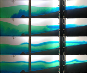
The development of the reflected waves is shown in figure 5 for a sequence of images that were spatially combined from the cameras imaging both red boxes shown in figure 2. Initially, the gravity current is propagating to the left of the image as it flows downslope, resulting in the lifting of the pycnocline at the left wall. After the pycnocline reaches its level of highest deflection (figure 5b), the built-up potential energy is converted back into kinetic energy and the system relaxes, resulting in a low-frequency surge of the lower layer to the right, followed by higher frequency internal waves (figure 5c,d), also propagating to the right. These waves were observed to be nonlinear and their shape continued to evolve as they continuously interacted with the topographic slope as they progressed. In the lowest  $Ri_{\rho }$ cases, Kelvin–Helmholtz instabilities were observed along the pycnocline resulting from the shear across the interface driven by the surge of the ambient layers, as the launched wave may still be propagating to the left at this point. Both the surge and the internal waves cause fluid to be displaced above its level of neutral buoyancy, providing opportunities for mixing via gravitational instabilities. The internal waves are then observed to break on the slope (figure 5d), providing another possible mechanism for mixing. The surge is observed to propagate across the length of the tank multiple times before its motion is dissipated.

Figure 5. Experimental images from two combined cameras showing the progression of the gravity current and pycnocline response for  $Ri_{\rho }=1.55$ (run 1-V). Snapshots are shown for
  $t=32$ s (a), 43 s (b), 70 s (c) and 99 s (d).
4.2. Temporal response of the pycnocline
As the deflected pycnocline starts to return to its neutral level, the phenomena we observe are similar to those reported by Boegman et al. (Reference Boegman, Ivey and Imberger2005a) where a tilting tank was used to set up an initial pycnocline deflection and then was returned to its original position, to replicate what occurs to a stratified system once a sustained wind stress is removed, as discussed in § 2. The top panel in figure 6 shows the temporal response of the pycnocline, extracted using the PLIF virtual wave gauge technique described above, at a position 20 cm downstream from where the pycnocline originally met the slope. Initially, the pycnocline is deflected upwards and downwards due to the underflow portion of the gravity current passing beneath the pycnocline. At 43 s ( $t/T_i=1$), the low frequency surge manifests as a long-period wave, followed by higher frequency internal waves. After the initial 5–7 waves, internal waves are no longer observed at the wave gauge, but the lower frequency signal does persist.

Figure 6. Temporal response of the pycnocline (a) positioned 20 cm downstream from where the pycnocline originally meets the slope obtained from a virtual PLIF wave gauge, and the associated continuous wavelet transform (b) where the colours indicate the power spectral density (PSD), for  $Ri_{\rho }=2.06$ (run 2-P).
The amplitude of these internal waves was measured where the internal waves were first generated, near the base of the slope where the water depth was constant. Figure 7 shows the amplitude  $(a_w)$ of the first wave (the low frequency surge) normalized by the upper layer height
  $(h_1)$ as a function of the initial Richardson number. Generally, we find that a lower
  $Ri_{\rho }$ leads to a higher wave amplitude due to the higher deflected momentum of the larger underflow. For lower
  $Ri_{\rho }$ the dominant wave generation mechanism is the interaction between the locked wave and the underflow with the back wall of the tank, though subsequent measured waves are a superposition of the generated waves and the launched wave that arrives later. The observed trend is also similar to previous observations by Monaghan et al. (Reference Monaghan, Cas, Kos and Hallworth1999) in their figure 5, who also found the relationship between the wave amplitude and gravity current strength to hold across a range of topographic slopes.

Figure 7. Normalized amplitude of the first observed internal wave as a function of  $Ri_{\rho }$.
Figure 6(b) shows the continuous wavelet transform of the time series shown in figure 6(a), computed using the jLab analysis package (Lilly Reference Lilly2021). Because the wavelet basis functions are not orthogonal, specific amplitudes cannot be attributed to specific frequencies, but trends of the energy containing frequencies can be inferred from the continuous wavelet transform. A low frequency mode (that we identify as the surge) with a period between  $T_i$ and
  $T_i/2$ can be observed, with a strong signal from approximately 43 s (
 $t/Ti=1$) until approximately 258 s (
 $6T_i$). This period is similar to that observed in the continuous wavelet transform computed by Boegman et al. (Reference Boegman, Ivey and Imberger2005a) in their figure 4. The higher frequency internal waves observed in figure 6 between 65 s (
 $1.5T_i$) and 129 s (
 $3T_i$) have a period of around
  $Ti/4$ to
  $Ti/8$, which can be compared with the solitary waves observed by Boegman et al. (Reference Boegman, Ivey and Imberger2005a), which had a period closer to
  $Ti/16$. In general, the frequencies associated with the packet of solitary waves generated by the evolution of the surge observed by Horn et al. (Reference Horn, Imberger and Ivey2001) and Boegman et al. (Reference Boegman, Ivey and Imberger2005a) were higher than the frequencies of the waves generated here after the initial surge (in terms of
  $T_i$). The waves in this time frame are propagating to the right, and continue to steepen as they interact with the bottom topography. One difference between the solitary waves of Boegman et al. (Reference Boegman, Ivey and Imberger2005a) and the waves observed here is the generation mechanism. The solitary waves in Boegman et al. (Reference Boegman, Ivey and Imberger2005a) arose from the evolution of the surge through steepening, whereas the waves here were generated separately following the surge. In the experiments of Boegman et al. (Reference Boegman, Ivey and Imberger2005a) the layer heights were much more unequal, a stronger baroclinic initial forcing was applied, and the horizontal pycnocline length was longer. All of these factors contributed to increased wave steepening and nonlinearity resulting from the initial surge, as explained by the theory derived by Horn et al. (Reference Horn, Imberger and Ivey2001) and Boegman et al. (Reference Boegman, Ivey and Imberger2005a,Reference Boegman, Ivey and Imbergerb). These factors, in addition to the higher level of stratification supporting higher frequency motions, may explain the observed differences. The energy in the high frequency band drastically drops off after approximately 170 s (
 $4T_i)$, due to the internal waves shoaling and breaking on the slope, consistent with previous observations in experiments with inclines.
After the high frequency internal waves dissipate, there are small nodules that travel across the pycnocline, like beads on a string, which manifest as small amplitude oscillations in the time series in figure 6(a) after 200 s ( $5T_i$) or so, for example. The initial head of the intrusion of the interflow portion of the gravity current reflecting from the back wall appears to be the first nodule ( figure 8a, red solid arrow), similar to the gravity current in figure 4 of Maxworthy et al. (Reference Maxworthy, Leilich, Simpson and Meiburg2002). The structure of these nodules is similar to the intrusive gravity currents observed by Lowe, Linden & Rottman (Reference Lowe, Linden and Rottman2002), though they lack the highly dissipative wake region behind the head. The structure is also similar to the undular bore case in figure 13.11 in Simpson (Reference Simpson1997) where the head has detached from the following flow and no mixing is observed across the interface. Finally, the absence of Kelvin–Helmholtz instabilities developing on either side of the nodules is consistent with the observations of Britter & Simpson (Reference Britter and Simpson1981) where mixing between the intrusion and the ambient fluid ceases when the thickness of the interface and the intrusion become comparable.

Figure 8. Experimental snapshots of  $Ri_{\rho }=1.55$ (run 1-V) showing the formation of nodules along the pycnocline. Red solid and blue hollow arrows indicate certain nodules observed in the flow. The snapshots are at
  $t=81$ s (a), 135 s (b), 153 s (c) and 183 s (d).
In the present case, subsequent nodules appear to be generated after the internal surge progresses up the slope (right-hand side in figure 8a) and the fluid mixed at the front of the surge recedes downslope, generating a nodule of fluid with momentum along the pycnocline (figure 8b blue hollow arrow). As these nodules traverse the pycnocline (figure 8c), they appear to pass through each other, though some amount of interaction is observed where one nodule appears to traverse above the other (figure 8d).
4.3. Bolus formation and breaking
4.3.1. Bolus classification
The high frequency waves are absent from the time series and continuous wavelet analysis after the first 5–7 waves are observed, and the time series does not show signs of reflection as the waves break on the slope. A time progression of an internal wave breaking event is shown in figure 9 for  $Ri_{\rho }=1.96$. As the first internal wave is about to break (figure 9a), the internal surge is receding. As the second wave is about to break in figure 9(b), the receding surge has produced a thin shear layer flowing downslope (indicated by the white arrow in figure 9b), causing the wave to break as a forward breaker (figure 9c), using the classifications of internal waves breaking on a slope as defined by Moore, Koseff & Hult (Reference Moore, Koseff and Hult2016). At the time the third wave is expected to break (figure 9d), the fluid from the first two waves is starting to flow downslope. Combined with the shear layer from the receding surge, the fluid at the slope is flowing strongly downslope, inhibiting the formation of a coherent bolus and resulting instead in a turbulent surge (Moore et al. Reference Moore, Koseff and Hult2016).

Figure 9. Experimental snapshots of wave breaking for  $Ri_{\rho }=1.96$ (run 4-V), at
  $t=106$, 117, 121 and 129 s. The lower layer surge is seen receding during this time.
The phase and period of the surge was also observed to affect the wave-breaking process. Figure 10 shows a sequence of an internal wave-breaking event for  $Ri_{\rho }=3.32$, a case in which less of the initial gravity current results in an underflow. The first wave is breaking in figure 10(a), the second wave is breaking in figure 10(b) and the surge is receding between these first two frames. However, as the third wave is about to break, the lower layer surge returns, visible from the increase of the green lower layer fluid to the right of the support column between figures 10(c) and 10(d), indicated by the white arrows. The upward surge now carries the would-be bolus fluid upslope, drastically changing the wave-breaking process.

Figure 10. Experimental snapshots of wave breaking for  $Ri_{\rho }=3.32$ (run 6-V) at
  $t=114$, 127, 137 and 146 s. The lower layer surge is receding in panels (a–c) but is progressing in panel (d), affecting the wave breaking.
4.3.2. Bolus propagation speed
The average bolus propagation speed  $C_{avg}$ is shown in figure 11, where the speed has been normalized by a characteristic wave velocity
  $\omega a_w$, where the incoming wave frequency
  $\omega$ and amplitude
  $a_w$ are extracted from Hovmoller diagrams obtained by processing the images from the tracer dye experiments. In figure 11(a), the bolus speeds are plotted against the wave Froude number defined by Moore et al. (Reference Moore, Koseff and Hult2016) as
 \begin{equation} Fr=\frac{\omega a_w}{c_0}. \end{equation}
Similarly, in figure 11(b), the speeds are plotted against the wave steepness  $k a_w$, where
  $k$ is the wavenumber. Although, as discussed previously, the boundary conditions for breaking are greatly modified by the internal surge and the downslope boundary flow, the bolus speed follows the same trends observed by Moore et al. (Reference Moore, Koseff and Hult2016). At high wave forcings of
  $Fr>0.2$ and
  $k a_w>0.35$, the average bolus speed asymptotes to the characteristic velocity scale
  $\omega a_w$, consistent with the results of Moore et al. (Reference Moore, Koseff and Hult2016) and noted as a point where the incoming wave energy shifts from the forward propagation of the bolus to the production of turbulence. Note that the average bolus speeds in the current study were not measured at the slope as in previous studies, but rather at a vertical location immediately above the thin shear layer created by the surge. The velocities of the boluses in the experiments were constant over time as they progressed upslope, consistent with previous observations by Venayagamoorthy & Fringer (Reference Venayagamoorthy and Fringer2007) and Moore et al. (Reference Moore, Koseff and Hult2016), suggesting that despite the change in the bottom boundary condition, the forward momentum imparted from the internal wave and the bottom shear quickly reaches a steady-state balance.

Figure 11. Normalized average bolus propagation speeds plotted against wave Froude number and wave steepness (red), along with experimental data from Moore et al. (Reference Moore, Koseff and Hult2016) (blue), reproduced with permission.
4.4. Mixing due to reflections and breaking waves
4.4.1. Change in density structure
In the absence of any horizontal gradients or motion, the potential energy of the tank can be calculated from the vertical density profile following the approach of Ivey & Nokes (Reference Ivey and Nokes1989) and Michallet & Ivey (Reference Michallet and Ivey1999), as
 \begin{equation} PE=g \int_z z A(z) \rho(z)\,\textrm{d}z \end{equation}
so that the change in potential energy for a density profile before ( $\rho _{initial}$) and after mixing events (
 $\rho _{final}$) can be expressed as
 \begin{equation} \Delta PE = g \int_z z A(z) (\rho_{final}-\rho_{initial}) \,\textrm{d}z \end{equation}
where  $A(z)$ is the horizontal cross-sectional area of the tank at a given height. Using an initial density profile taken before the release of the gravity current and a final profile taken at the end of the experiment, we calculate the total change in potential energy in the experiment due to the gravity current fluid intrusion, reflections and internal wave breaking, all manifest as a change in the pycnocline thickness, by this method.
As discussed in Hult et al. (Reference Hult, Troy and Koseff2011a), obtaining a reliable estimate of  $\Delta PE$ from numerically integrating a measured profile is difficult, due to noise and possible drift of the probe. In addition, in the present experiments, some of the gravity current fluid will be introduced into the bottom of the water column as an underflow, displacing the pycnocline, and carrying out the numerical integration of the density profile would result in a much higher potential energy compared with the initial profile due to this upward displacement. To avoid these complications, we turn to the approach used by Hult et al. (Reference Hult, Troy and Koseff2011a) and fit an error function of the form
 \begin{equation} \rho(z)=\rho_0 - \frac{\rho_2 - \rho_1}{2} \textrm{erf}(\beta z) \end{equation}
to the initial and final profile (for densities less than or equal to that of the lower layer) using a standard nonlinear fitting algorithm (MATLAB nlinfit). The error associated with fitting the density profile was extremely low, with  $r^2$ values consistently higher than 0.96. The 95 % confidence intervals of the pycnocline thickness and position were also propagated in subsequent calculations. The length scale
  $\beta ^{-1}$ can be related to the 99 % thickness of the interface as defined by Troy & Koseff (Reference Troy and Koseff2005) and Fringer & Street (Reference Fringer and Street2003), using the relation
  $\delta =3.64 \beta ^{-1}$. By substituting (4.4) into (4.3), the integral and change in potential energy can be calculated numerically.
Although the gravity current underflow is the only way to introduce a fluid denser than the lower layer fluid into the water column, there are multiple pathways to generate fluid of intermediate density between those of the upper and lower layers and thus change  $\beta _{final}$. As the gravity current splits into an underflow and an interflow, the part that is introduced at the pycnocline will increase the thickness of the interface. Furthermore, as reflections and the generated internal waves break on the slope, the resulting mechanical mixing can also generate more fluid of intermediate density and thus alter the density structure. However, with knowledge of only the density profiles at the beginning and at the end of experiment, it is not possible to apportion the change in potential energy between these two contributing sources.
To resolve the change in potential energy due to the mechanical mixing from wave breaking, we must measure a density profile before the internal waves have broken but after the gravity current has split into an interflow and underflow, using PLIF. Previous experiments with internal waves generated on a thin two-layer interface, such as those of Michallet & Ivey (Reference Michallet and Ivey1999), Troy & Koseff (Reference Troy and Koseff2005) and Hult et al. (Reference Hult, Troy and Koseff2011a), were able to capture an initial density profile using a conductivity probe prior to any wave generation as well as a final profile at a time after all horizontal gradients had dissipated, but prior to when viscous diffusion had thickened the interface. Density profiles obtained at the start of the experiment from PLIF and the CT probe shown in figure 12 show good agreement, apart from a small deviation in the upper portion of the pycnocline in the PLIF profile. This deviation does not affect the results as the density profiles are fitted to an error function. There is a small ‘knee’ in the top of the lower layer in the baseline profile obtained by the CT probe most likely due to the differences in response times between the on-board thermistor and conductivity sensor. The resulting unstable density is an artefact of the probe, and not an actual unstable density configuration prone to gravitational instabilities. These kinds of erroneous readings typically occur when sharp density gradients are present, but are not present when the interface thickens. In the present case, we need to rely on the PLIF density measurement to obtain a profile prior to wave breaking during the experiment. As there is continuous motion along the interface during this time where a density profile needs to be obtained, we use the average thickness of the pycnocline during the initial largest amplitude internal waves (typically three wave periods). An example of a profile acquired by PLIF in this time is given in figure 12, and an explanation of the temporal variability of the interface thickness in the presence of internal waves is given in § 5.2.

Figure 12. Normalized density profiles obtained for  $Ri_{\rho }=1.61$ (run 1-P), centred around the vertical location of the interface. The initial profile prior to breaking is taken with PLIF at
  $t=106$ s, and the final profile with the CT probe two hours after the experiment.
The final profile is acquired using the conductivity probe when the tank is at a quiescent state with no horizontal gradients. To avoid any possible contamination of the vertical profile due to nodules in the interface, multiple profiles are taken to ensure that all motion has ceased, at least two hours after the initial release of the gravity current. As shown in figure 12, the final profile shows a larger pycnocline thickness as compared with the initial profile prior to breaking, as well as a vertical displacement of the pycnocline due to the gravity current underflow compared with the profile at the beginning of the experiment. Using this final profile and the initial density profile before the experiments allows the calculation of the overall total change in potential energy during the experiment. The final profile along with the intermediate-time profile obtained from PLIF allows for the calculation of the change in potential energy due to the mechanical mixing from the wave-breaking events. The ratio of the wave-induced change in potential energy to the total change in potential energy varied from 1 % to 53 % with a mean of 27 %; however, we observed no trend with  $Ri_{\rho }$. This result suggests that the mixing due to the wave activity can be a significant factor in changing the potential energy of the system, but that the fraction of the mixing due to the waves is seemingly independent of
  $Ri_{\rho }$.
4.4.2. Mixing efficiency
With internal wave breaking, we can also use the vertical density structure and pycnocline position time series to calculate the overall mixing efficiency,  $R_{f,o}$, of the breaking events, following the procedure of Hult et al. (Reference Hult, Troy and Koseff2011a) and using the tank as a control volume. The calculation consists of determining the change in potential energy due to the wave-breaking events (see § 4.4.1) and then calculating the work done due to the wave energy from the time integrated signal of the internal waves. In the following sections we outline the methodology of each of these steps.
(i) Work done due to wave energy.
The wave energy can be calculated from the time series of the interfacial displacement from the PLIF images as
 \begin{equation} WE=c_p g \Delta\rho \int_{t_1}^{t_2} \eta_{wave}^2 (t) \,\textrm{d}t, \end{equation}
where  $c_p$ is the phase speed of the wave, assuming an equal partitioning between the potential and kinetic energy of the wave (Bogucki & Garrett Reference Bogucki and Garrett1993). The assumption of equal partitioning is valid in the case where the pycnocline is near the midheight of the water column, where the ratio of the potential and kinetic energies has been shown to be between 1 and 1.01 (Lamb & Nguyen Reference Lamb and Nguyen2009). The phase speed is measured directly by placing two virtual wave gauges with a known spatial separation at the edges of the PLIF images and using the interfacial displacement time series from each. The measured phase speeds ranged from
  $c_p/c_0=0.58$ to 0.64 with no clear trend with
  $Ri_{\rho }$, with a mean of 0.61, lower than the long wave limit. The bounds of integration,
  $t_1$ and
  $t_2$, are chosen such that
  $\eta _{wave}(t_1)=\eta _{wave}(t_2)=0$, consistent with Michallet & Ivey (Reference Michallet and Ivey1999), among others.
The time series of the interfacial displacement derived from PLIF in figure 6 is not due only to the wave signal, but rather is the summation of the wave and the internal surge of the lower layer. Thus, we decompose it as
 \begin{equation} \eta(t)=\eta_{wave}(t) + \eta_{surge}(t) \end{equation}
and use the wave signal to compute the incoming energy to the incline. From the continuous wavelet analysis in figure 6(b) as well as visual inspection of the full time series, it is evident that the internal waves and surge have different characteristic frequencies. We thus follow the spectral filtering approach of Boegman et al. (Reference Boegman, Ivey and Imberger2005a) and use a low-pass, second-order Butterworth filter with a cutoff of  $f=3/2 T_i$ to remove the surge component from the full signal, with the residual then being the desired wave signal. Figure 13 shows the different components from the spectral filtering, based on the interfacial displacement obtained from PLIF. The extracted surge signal (dashed, green line) has a much lower frequency as compared with the high-frequency wave time series (dash–dot, blue line), and roughly one surge period is present during the initial series of internal waves from 75 s to 125 s. The mean of the wave signal after the passing of the surge was very close to zero, as the spectral filtering was effective in differentiating the two signals. The amplitude of the waves are often proportional to the amplitude of the initial surge shown in figure 7, and the wave energy calculated by (4.5) generally was seen to decrease with increasing
  $Ri_{\rho }$.

Figure 13. Time series of different interfacial displacement components using the spectral filtering method of Boegman et al. (Reference Boegman, Ivey and Imberger2005a), for  $Ri_{\rho }=1.61$ (run 1-P). The original displacements are obtained from PLIF.
(ii) Overall mixing efficiency.
The overall mixing efficiency for a packet of internal waves is computed as the change in potential energy resulting from the work input of the internal waves, or
 \begin{equation} R_{f,o}=\frac{\Delta PE}{WE}. \end{equation}
 The calculated  $R_{f,o}$ over the entire Richardson number range varies from
  $0\text {--}0.05 \pm 0.01$. There is no observable trend with
  $Ri_{\rho }$ rather,
  $R_{f,o}$ is constant over the experiments with a relatively low value. The relatively low mixing efficiency can be compared with the mixing efficiencies from other experiments and computations involving breaking waves on slopes (see table 2), and is discussed in more detail in § 5.
Table 2. Comparison of overall mixing efficiencies from previous studies. DNS, direct numerical simulation.

5. Discussion
5.1. Characterization of the reflections
Given the similarities between this flow and that generated by surface shear due to wind, the question arises as to whether something like a Wedderburn number can be used to characterize the behaviour of the reflections in our flow. The maximum pycnocline deflection at the end of the tank was measured from the imaging with the tracer dye. Because the back of the tank was lit fairly uniformly, a Hovmoller diagram can be extracted from the images and a simple gradient detection method can be employed to determine the position of the pycnocline, denoted by the red line in figure 14.

Figure 14. Hovmoller diagram of a transect from the back wall of the tank for  $Ri_{\rho }=1.96$ (run 4-V), the pycnocline location is denoted in red.
While the ratio of the maximum pycnocline deflection to the top layer height is similar to the inverse of the Wedderburn number given in (2.6), an exact analogy cannot be made because the Wedderburn number describes the basin-scale pycnocline tilt from wind shear. In our case, the tilted pycnocline arises from a displacement of the pycnocline from the plunging gravity current. Consequently, to acknowledge the inherent differences in the tilt generation mechanisms, we refer to this number as  $W_{GC}$, and
  $W^{-1}_{GC}$ is computed with (2.6). Figure 15 shows the Richardson number of the gravity current plotted against
  $W^{-1}_{GC}$ for each experimental case. Tanimoto et al. (Reference Tanimoto, Ouellette and Koseff2020) previously showed that
  $Ri_{\rho }$ predicts the degree of splitting of the gravity current into underflow and interflow components. We would, therefore, expect that with increased underflow (lower
  $Ri_{\rho }$), we should see a stronger pycnocline deflection and, therefore,
  $W^{-1}_{GC}$; this is indeed what figure 15 shows. A least-squares linear fit of the data gives
  $r^2=0.98$, suggesting that
  $W^{-1}_{GC}$ for our system is a linear function of the forcing, characterized by
  $Ri_{\rho }$. As seen in figure 7, however, the initial surge amplitude is not as linear with respect to
  $Ri_{\rho }$ as
  $W^{-1}_{GC}$ is, because the initial interaction of the gravity current and the pycnocline results in two waves (Tanimoto et al. Reference Tanimoto, Ouellette and Koseff2020).

Figure 15. Here  ${W^{-1}_{GC}}$ plotted as a function of the initial Richardson number of the gravity current (
 $Ri_{\rho }$). Errors propagated from the uncertainty in the measurements are smaller than the symbol size.
From our current experiments, we cannot determine how generalizable this parameterization is because the effect of the length of the basin on the baroclinic response needs to be investigated. Specifically, for the same  $Ri_{\rho }$, we would expect that
  $W^{-1}_{GC}$ will decrease as the length of the basin increases (holding all other variables constant), since the locked wave due to the underflow or the launched wave will be arrested by viscous forces in longer basins, thus reducing the magnitude of the baroclinic response at the basin wall. Thus, more experiments to quantify the baroclinic response with basins of different lengths but the same forcing mechanisms are needed. The time or length scales over which the motions generated by the gravity current will vary should be a function of
  $Ri_{\rho }$ and the dominant wave regime identified by Tanimoto et al. (Reference Tanimoto, Ouellette and Koseff2020). For low
  $Ri_{\rho }$, the time until the gravity current is arrested will be a function of the viscous bottom drag and entrainment of the quiescent ambient layer, and for higher
  $Ri_{\rho }$ the time until motions cease may potentially be predicted by the viscous theory of Troy & Koseff (Reference Troy and Koseff2006), for example.
If the upper layer height were reduced in our experiments, we expect the following to occur. A shallower upper layer will lead to less entrainment of the ambient fluid by the gravity current and a corresponding decrease in  $Ri_{\rho }$, leading to more of the gravity current fluid entering the bottom of the water column as an underflow. This in turn will lead to more elevated pycnocline at the back wall, resulting in a higher
  $W^{-1}_{GC}$ (a result that is consistent with figure 15). Complete upwelling (
 $W^{-1}_{GC}=1$) is possible at low
  $Ri_{\rho }$ when the pycnocline reaches the free surface, but as the pycnocline cannot penetrate the free surface,
  $W^{-1}_{GC}$ will saturate for lower
  $Ri_{\rho }$. A thinner upper layer would also change the wave dynamics, as the dispersion relation for interfacial waves in a two-layer stratified system depends on the heights of each of the two layers, and could also change the wave breaking at the slope. Our expectation, however, is that in relatively short confined basins, dense gravity currents are in fact likely to induce a baroclinic system response. As the basin length increases, more of the momentum of the gravity current along with any generated internal motions will be dissipated by viscous forces.
While a general parameterization of the baroclinic response from a dense gravity current is difficult to derive, Horn et al. (Reference Horn, Imberger and Ivey2001) previously identified the expected dominant phenomena in wind-forced stratified systems for different inverse Wedderburn numbers and normalized pycnocline depths,  $h_1/H$, where
  $H$ is the full height of the water column. The forcing mechanism in the present experiments is different from those used by Horn et al. (Reference Horn, Imberger and Ivey2001) in deriving this theory, however, there are consistencies between the predicted theory and the observed baroclinic response from a gravity current. In the present experiments, the measured
  $W^{-1}_{GC}$ ranged from 0.2 to 0.67, and
  $h_1/H$ was fixed at 0.43, falling in regime 1 according to figure 2 of Horn et al. (Reference Horn, Imberger and Ivey2001) where damped basin-scale waves are expected, as was observed. The present experiments do not show the transformation of the surge into solitary waves, which is consistent with the theory presented in Boegman et al. (Reference Boegman, Ivey and Imberger2005b) that the nonlinear coefficient diminishes as the height of the original interface approaches the mid-depth of the water column. In the situation mentioned previously where the layer heights are made more unequal, the theory of Boegman et al. (Reference Boegman, Ivey and Imberger2005b) predicts that this nonlinear coefficient will increase, hence the surge will undergo nonlinear steepening to evolve into solitons.
Although field observations of this phenomenon are sparse, Brizuela et al. (Reference Brizuela, Filonov and Alford2019) observed a submarine landslide that induced internal seiches with a period close to that of the fundamental period in a stratified lake, followed by high-frequency internal waves. Brizuela et al. (Reference Brizuela, Filonov and Alford2019) also reported that the gravity current traversed across the basin eight times, which allowed it to continue to generate and drive internal motions long after the initial event. Based on the data from their figures 2 and 3, it can be estimated that  $W^{-1}_{GC}=0.2$ and
  $h_1/H=0.2$, not too dissimilar to the current experiments, suggesting that the current framework and parameterization is applicable to their case as well.
5.2. Interface thickness
The effect of varying pycnocline thicknesses on wave forcing has not been studied extensively in the laboratory, and the effects are not fully known. We observed from the PLIF images that the pycnocline thickness changed in phase with the pycnocline deflection, and that the interfacial thickness was not constant in the presence of internal waves, as shown in figure 16. Although this is not the focus of the present study, we offer one possible explanation for these phenomena here. A thick interface will behave as a many-layered system with multiple densities in a stable configuration. At the crest of an internal wave, all of the layers will be elevated, but to an unequal degree due to the different densities, resulting in a spreading of the stacked layers and a thicker pycnocline. At the trough of a wave, the different layers will be accelerated downward and assisted by gravity, resulting in a thinning of the pycnocline beyond its natural thickness. So as not to bias our estimates of the thickness of the initial profile, we computed an averaged thickness over the first three wave periods. After this time, the intermediate fluid resulting from the breaking waves starts to recirculate back into the PLIF measurement domain.

Figure 16. Time series of the interface deflection and thickness from PLIF for  $Ri_{\rho }=1.61$ (run 1-P).
5.3. Mixing efficiency
The overall mixing efficiency of 0–0.05 is relatively low compared with previously measured values from laboratory experiments and numerical simulations, listed in table 2. Even so, however, we argue that these values provide an upper bound on the efficiency of the system. The calculation of the overall mixing efficiency by measuring the change in potential energy hinges on the physical assumption that the wave energy causing irreversible mixing is the only pathway to generate more intermediate density fluid in a two-layer interfacial wave system.
Some additional assumptions that were necessary to perform the analysis are discussed here. First, the initial vertical profile density profile was used to establish the baseline potential energy in the tank before any wave-breaking events caused mixing. We measured it using a conductivity probe before the generation of internal waves, as in the experiments of Michallet & Ivey (Reference Michallet and Ivey1999), Hult et al. (Reference Hult, Troy and Koseff2011a) and others. This approach assumes that a single vertical profile of density can be used to characterize the potential energy using the tank as a control volume, an assumption valid in the absence of any motion and lateral density gradients. In the present experiments, however, the flow is more complex and this assumption breaks down. As the waves approach the slope, the interface thickens due to recirculation by the internal wave field, so that the interface thickness is different near the slope and off the slope. In computing the initial  $\beta$, we used an average thickness over the first few waves as in § 5.2, but perhaps a more representative measure would be a weighted average of the pycnocline thickness across the entire tank. However, this would require a measurement of the pycnocline thickness at all points in the tank, which is difficult to obtain in most laboratory settings. Recalculating the overall mixing efficiency using the maximum
  $\beta _{initial}$, and thus the thinnest interface thickness observed, yielded efficiencies of 0.03–0.06 – still relatively low, but a more extreme upper limit on the efficiency of our system. Propagating the 95 % confidence intervals for the pycnocline position and thickness through the mixing efficiency calculations yielded differences much smaller than differences computed from assessing the temporal fluctuations of these parameters.
Second, the final density structure is more readily obtained from a density profile measured once all motion has ceased in the tank, again assuming that the change in potential energy results solely from the mixing due to breaking waves. While molecular diffusion plays a part in thickening the interface, it is only significant after much longer times and so it is reasonable to neglect it. Third, in the present experiments, the surge generated nodules that traverse the pycnocline; by the time the final profiles were taken, however, the nodules had all disappeared due both to viscous dissipation and hydrostatic pressure. The intermediate density fluid generated from the surge would also add to the interfacial thickness measured in the final density profile. Thus, computing the change in density solely from the nodules is extremely difficult due to the number of nodules traversing the pycnocline and because these nodules also interact with the topographic slope and may generate small-scale boluses themselves.
The wave energy is calculated from (4.5), and considers the work done by the internal waves. As shown in Troy & Koseff (Reference Troy and Koseff2006), sidewall friction can play a key role in viscous damping of the wave energy, along with bottom boundary friction. These effects are to some degree captured in the current formulation, as the wave energy is extracted from the PLIF imagery at a location prior to steepening but close to the breaking site. Any energy loss due to friction, therefore, would have already affected the waves, and would be captured in the measured wave signal. What our formulation does not account for, however, is the energy imparted by the lower layer surge, possibly resulting in an underestimate of the work done by the waves. As the surge progresses up the slope, fluid is continuously displaced above its level of neutral buoyancy, and the surge provides opportunities for both shear-induced mixing and gravitational instabilities, which are not accounted for in our calculation of the work.
Taking all the points in the above discussion together, we have possibly overestimated  $\Delta PE$ and underestimated
  $WE$ in our
  $R_{f,o}=\Delta PE/WE$ calculation and, therefore, we expect the efficiency we have reported to be an overestimate. Compared with values reported from the previous studies listed in table 2, however, our efficiency appears to be relatively low.
There are a number of possible reasons for this. First, compared with the deep water breaking events of Fringer & Street (Reference Fringer and Street2003) as discussed in Hult et al. (Reference Hult, Troy and Koseff2011a), a lower mixing efficiency is somewhat expected in a topographically induced breaking event where the wave flow is focused along the topographic boundary instead of being focused along the interface, where it can result in mixing. Second, it is also possible that the turbulence generated by the breaking is concentrated in areas without density gradients, as was the case in Hult, Troy & Koseff (Reference Hult, Troy and Koseff2011b). Examination of this possibility would require simultaneous measurements of the velocity and density fields, which we do not do in these experiments.
A third possible reason is the intense shear at the bottom boundary (due to the receding surge). Before the turbulence generated by the forward breaking is able to cause mixing, much of the fluid is transported off the slope, and so the resultant mixing tends to be concentrated along the interface instead of mixing the lower layer fluid from the bolus with the upper layer as in a typical wave-breaking event. In some cases, such as  $Ri_{\rho }=1.96$ in figure 9, the second break does not occur before the fluid is well away from the slope. Fourth, with breaking internal waves, there is a secondary recirculation pattern established that also transports fluid off the slope, resembling the formation of an intermediate nepheloid layer (Arthur & Fringer Reference Arthur and Fringer2016; Masunaga et al. Reference Masunaga, Arthur, Fringer and Yamazaki2017). Based on observations from our experiments, this recirculation pattern appears to affect and reduce the mixing due to the internal waves by recirculating the receding surge fluid (mostly comprised of the lower layer density) into the interface after the first few waves, thus causing a thickening of the pycnocline and affecting the nature of the following breaking events, as also reported by Moore et al. (Reference Moore, Koseff and Hult2016). This process, which results in the removal of the bolus fluid (prior to mixing) by the receding surge, appears to be the main mechanism responsible for the low mixing efficiency.
There are also other considerations when comparing the mixing efficiency to values reported from previous experiments. For example, Michallet & Ivey (Reference Michallet and Ivey1999) showed that the efficiency is a function of the ratio of the length scale of the wave to the length scale of the slope. At low ratios, the efficiency is low due to viscous forces being dominant over the mild slope, while at high ratios, a greater proportion of the incoming energy is reflected, again lowering the efficiency. The peak efficiency of 0.25 was measured at a wave-to-slope ratio of approximately 0.5. However, the experiments of Michallet & Ivey (Reference Michallet and Ivey1999) had much greater ratios of the lower layer to the total water depth and density ratios of the two layers, and also measured the mixing from a sole internal solitary wave. Thus, their experiments and conditions are somewhat dissimilar to the present study. A direct comparison of the results would be more appropriate if the ratio of the top and bottom layers were modified in the current setting. Then, if the framework proposed by Horn et al. (Reference Horn, Imberger and Ivey2001) holds as previously discussed, a gravity current could produce more nonlinear waves from the initial surge, similar to those observed by Boegman et al. (Reference Boegman, Ivey and Imberger2005a,Reference Boegman, Ivey and Imbergerb), and the interaction of these waves with the topography would increase the potential for mixing. Past results from Moore et al. (Reference Moore, Koseff and Hult2016) also show that wave breaking will be greatly altered by the change in the interface thickness, which is unavoidable as a gravity current splits into underflow and interflow. A gravity current entering a stratified environment will insert itself into multiple levels of neutral buoyancy, and with it will also trigger motions at multiple time scales, adding complexity to the system. These complexities are absent in other experiments were the primary scope of the work was purely to measure the mixing efficiency of breaking internal waves.
6. Conclusions
We used laboratory experiments to study the dynamics of a dense gravity current flowing down an incline into a quiescent two-layer stratification in a confined basin and the subsequent generation of an internal surge and internal waves. Although the generation of internal waves in stratified confined systems is often attributed to wind induced shear, our experimental observations show that dense gravity currents may also lead to the generation of internal waves. The perturbation of the interface initially is described by Tanimoto et al. (Reference Tanimoto, Ouellette and Koseff2020) and as the pycnocline deflection interacts with the back wall of the basin, the baroclinic response was observed to be similar to that resulting from a sustained wind forcing. Using a Wedderburn-like number to characterize the baroclinic response, we found that the response for our system is a linear function of the initial Richardson number of the gravity current.
Once the pycnocline relaxes, an internal surge was observed, followed by a train of nonlinear internal waves. The lack of evolution from the surge to a packet of solitary waves is consistent with predictions by Horn et al. (Reference Horn, Imberger and Ivey2001) and Boegman et al. (Reference Boegman, Ivey and Imberger2005a,Reference Boegman, Ivey and Imbergerb). Spectral analysis of the time series of the interfacial displacement showed that the energy was mainly contained in a persistent low frequency mode of the internal surge, and a more rapidly dissipating higher frequency mode in the form of the internal waves. The internal waves shoaled and broke upon encountering the topographic slope, which led the energy contained in the higher frequencies to dissipate quickly. The presence of the lower layer surge during the internal wave-breaking process led to forward-breaking boluses, following the classification scheme of Moore et al. (Reference Moore, Koseff and Hult2016). The surge changed the wave-breaking boundary condition at the slope to a strong, thin, shear layer, enhancing the downward flow caused by the initial wave typically observed in past internal wave-breaking experiments and simulations. In addition to the internal wave breaking, the surge introduced intermediate density fluid in the form of nodules that traversed the pycnocline, similar to the head of gravity current observed by Lowe et al. (Reference Lowe, Linden and Rottman2002) though lacking the tail portion.
The overall mixing efficiency of the internal waves was calculated using the tank as a control volume, following the approach of Hult et al. (Reference Hult, Troy and Koseff2011a). Although the calculation of both the change in potential energy and the work energy yielded an upper-bound estimate of the mixing efficiency, the value was found to be low compared with previous studies. Although more investigation and measurements are needed to determine the mechanism for this low value, it is most likely attributed to the lower layer surge changing the boundary conditions for breaking, and exporting the fluid that would mix with the upper layer after breaking away from the slope. The relatively low mixing efficiency of the breaking waves in the presence of the surge poses a question of the applicability of the mixing efficiencies of breaking waves computed in the laboratory and through idealized simulations, to confined basins settings or in the near coastal environment where internal wave breaking is not the only dynamical process occurring.
Acknowledgements
The authors thank B. Sabala for the fabrication of the experimental apparatus. We are also grateful for three anonymous reviewers for their thoughtful critique of the manuscript.
Funding
This work was supported by National Science Foundation Grant no. OCE 1634389.
Declaration of interests
The authors report no conflict of interest.


