


1. Introduction
1.1. The sphere wake as a model problem
The evolution of a sphere wake in a uniform density stratification is a convenient model problem to investigate the fluid dynamics of practical geophysical and nautical applications, such as the wakes generated by islands or the flow around submerged bodies. In addition to the Reynolds number,  $Re =\rho UL/\mu$, a second dimensionless group characterises the relative strength of stratification, known as the internal Froude number,
  $Fr = U/NL$, where
  $N^2 = -(g/\rho _0){\partial \rho }/{\partial z}$. Here,
  $U$ and
  $L$ are characteristic velocity and length scales in the flow,
  $\rho _0$ is a reference density,
  ${\partial \rho }/ {\partial z}$ is the density gradient,
  $g$ is the acceleration due to gravity in the direction of the density gradient and
  $\mu$ is the dynamic viscosity of the fluid. For the particular case of the sphere wake,
  $U$ and
  $L$ are taken as the body speed and diameter, respectively. The internal Froude number is
  $Fr = 2U/ND$, based on radius,
  $D/2$, so the value
  $Fr = 1$ denotes the maximum resonance between a convective time and a buoyancy time, as explained in § 2.3.
After some time, initially turbulent wakes evolving in a background density gradient develop a regular pattern of alternating vortices whose origin can be traced back to instabilities in the developing shear layers (Spedding Reference Spedding2002). The coherent structures emerge during what has been termed the non-equilibrium regime (NEQ) as the density gradient increasingly exerts an influence on the fluctuating and then mean vertical velocities. This period of adjustment of the wake to its background begins at approximately  $Nt = 2$, and ends at approximately
  $Nt = 50$, depending on the initial conditions. During this time, suppression of the fluctuating vertical velocity components reduces the associated Reynolds stress components and so decreases the kinetic energy dissipation rate (Brucker & Sarkar Reference Brucker and Sarkar2010; Redford, Lund & Coleman Reference Redford, Lund and Coleman2015). The vertical velocity fluctuations are diminished partly by the work required to lift fluid parcels from their equilibrium position, and partly because they can be removed from the wake as wake-generated internal waves. The energy contained in these waves, and removed from the wake, is an increasing fraction of the total as
  $Re$ increases (Abdilghanie & Diamessis Reference Abdilghanie and Diamessis2013; Rowe, Diamessis & Zhou Reference Rowe, Diamessis and Zhou2020) and high-resolution simulations in Watanabe et al. (Reference Watanabe, Riley, de Bruyn Kops, Diamessis and Zhou2016) demonstrated that the energy loss from wave radiation can be equal to the energy dissipated in turbulence in the wake itself.
1.2. The influence of initial conditions
After NEQ, the vortex motions persist. Streamwise averages of the mean and fluctuating velocities then yield statistically similar profiles in both lateral and vertical directions, and can be re-scaled based only on an effective drag coefficient (Meunier & Spedding Reference Meunier and Spedding2004, Reference Meunier and Spedding2006). In that case, the only amplitude variations come from the net horizontal momentum flux, and in all other respects the particular shapes have no far-wake influence. Instead, the dynamics is self-similar, much as the original hypothesis proposed by Townsend (Reference Townsend1976) for three-dimensional turbulent wakes. However, even in unstratified turbulent wakes, the hypothesis has been called into question in experiment (Bevilaqua & Lykoudis Reference Bevilaqua and Lykoudis1978; George Reference George1989) and in computations (Redford, Castro & Coleman Reference Redford, Castro and Coleman2012), which showed that differences in the wake structure far downstream could be traced back to differences in the initial conditions, affecting the evolution of mean and fluctuating quantities in differing ways.
Experiment and simulations agree on some approximate measures of the evolution of various length and velocity scales (Gourlay et al. Reference Gourlay, Arendt, Fritts and Werne2001; Dommermuth et al. Reference Dommermuth, Rottman, Innis and Novikov2002; Brucker & Sarkar Reference Brucker and Sarkar2010; Diamessis, Spedding & Domaradzki Reference Diamessis, Spedding and Domaradzki2011), but it is not easy to find general rules and predictions for when and how special features from initial conditions will prevent agreement. Early numerical simulations (Métais & Herring Reference Métais and Herring1989) indicated that stably stratified turbulence-in-a-box would retain memory of different initial conditions (such as balances of vortical vs internal wave motions). On the other hand, the widespread emergence of late-wake coherent structures and similar wake growth/decay rates in simulations having widely differing initialisations (Gourlay et al. Reference Gourlay, Arendt, Fritts and Werne2001; Dommermuth et al. Reference Dommermuth, Rottman, Innis and Novikov2002; Diamessis et al. Reference Diamessis, Spedding and Domaradzki2011; Redford et al. Reference Redford, Lund and Coleman2015) suggests that the particular route to the late wake may well be unimportant.
1.3. Scaling and turbulence in stratified wakes
A scale similarity in strongly stratified wakes has been demonstrated analytically by Billant & Chomaz (Reference Billant and Chomaz2001) who showed that, when  $Fr_h \ll 1$, a vertical length scale would be
  $l_v = U/N$, when energy is approximately equally partitioned between kinetic and potential energy. In that case a local Froude number based on vertical length scales and local fluctuating horizontal velocity,
  $u_h$,
  $Fr_v = u_h/N l_v = O(1)$. Lindborg (Reference Lindborg2006) showed that the
  $Fr_v = 1$ invariance can alternatively be demonstrated as a consequence following the stipulation of energy equipartition. The dynamics of stratified turbulence is ultimately determined by the relative magnitudes of turbulent, buoyancy and viscous dynamics. Spedding (Reference Spedding1997) proposed that turbulent stratified wakes evolve through three distinct regimes: a presumed three-dimensional (3-D) regime is initially unaffected by stratification, followed by a NEQ interval when buoyancy begins to significantly modify the dynamics then transitions into a flow state (Q2D) consisting mostly of 2-D motion, where the vertical velocity component,
  $w$, is small compared with
  $\{u,v\}$. The wake regime sequence of 3-D–NEQ–Q2D is based on wake-scale and mean quantities, which themselves are outcomes from local turbulence dynamics, as well as the initial forcing at
  $U$ and
  $D$. If we define local Reynolds and Froude numbers based on horizontal integral length scales,
  $l_h$, so
  $Re_h = u_h l_h/\nu$ and
  $Fr_h = u_h/N l_h$, then a combination of these yields a buoyancy Reynolds number,
 \begin{equation} \mathcal{R} = Re_h Fr_h^2, \end{equation}
the magnitude of which measures the range of scales over which horizontal turbulent motions can occur, even while being constrained by the condition of strong stratification, when  $l_v \ll l_h$ and
  $Fr_v = 1$. Lindborg (Reference Lindborg2006) showed that this kind of strongly stratified turbulence produces a forward energy cascade with horizontal wavenumber scaling of
  $k_h^{-5/3}$, as indeed measured in the atmosphere (Nastrom, Gage & Jasperson Reference Nastrom, Gage and Jasperson1984; Nastrom & Gage Reference Nastrom and Gage1985). Brethouwer et al. (Reference Brethouwer, Billant, Lindborg and Chomaz2007) extended the analysis to show that flows for
  $\mathcal {R} \gg 1$ are little affected by viscosity, and furthermore that within that regime there are two distinct sub-regimes. If we define an Ozmidov scale,
  $l_O = (\epsilon /N^3)^{1/2}$ as a scale where overturning motions are damped by stratification, and a Kolmogorov scale,
  $l_K = (\nu ^3/\epsilon )^{1/4}$, as a small scale where viscosity consumes turbulent fluctuations, then there is a range
  $l_K \leq l_t \leq l_O$ where turbulence can proceed mostly unaffected by either stratification or viscosity, and another range
  $l_t > l_O$ where energetic turbulence is nevertheless strongly influenced by buoyancy. In many laboratory experiments, especially at late times, size limitations lead to
  $\mathcal {R} \ll 1$ and Godoy-Diana, Chomaz & Billant (Reference Godoy-Diana, Chomaz and Billant2004) proposed that the observed independence of the late-time dynamics from
  $Fr$ can be understood as a limit when flows reach a viscous-dominated attractor, although relevant scaling laws for a
  $\mathcal {R} \gg 1$ state to reach the viscous regime could depend on the initial state.
Turbulence can occur in scales from  $l_K$ up to
  $l_O$, and de Bruyn Kops & Riley (Reference de Bruyn Kops and Riley2019) have drawn attention to a parameter we shall term
  $\mathcal {G}$, following early work by Gibson (Reference Gibson1980) and Gargett, Osborn & Nasmyth (Reference Gargett, Osborn and Nasmyth1984). Writing
  $l_O/l_K = \epsilon /N^2 \nu$, then since a root-mean-scale (r.m.s.) turbulent length scale can be written as
  $l_t = u_t^3/\epsilon$, the scale ratio is
 \begin{equation} \mathcal{G} = \frac{\epsilon}{N^2 \nu} = Re_t Fr_t^2, \end{equation}
where  $Re_t$ and
  $Fr_t$ are based on the r.m.s. turbulent velocity,
  $u_t$ and
  $l_t$;
  $\mathcal {G}$ was described as an activity parameter in de Bruyn Kops & Riley (Reference de Bruyn Kops and Riley2019) and together with a local Froude number, its value can be used to separate dynamically dissimilar regimes as an initial turbulence decays against a stratified background. The expressions in (1.1), (1.2) depend on
  $l_h, u_h$ and
  $l_t, u_t$, respectively, where
  $u_h$ is an r.m.s. velocity scale in the horizontal and
  $u_t$ is the total r.m.s. velocity. The ratio of
  $\mathcal {G}/\mathcal {R}$ varies with time, and with
  $Re$ (de Bruyn Kops & Riley Reference de Bruyn Kops and Riley2019). The relationships between a dissipation rate,
  $\epsilon$ and other length and velocity scales is readily supported in strong, box-filling turbulence, but less clear in weaker turbulence that evolves in highly anisotropic fashion from its start. Wakes are also non-uniform in space, and measures such as
  $\mathcal {G}$ and
  $\mathcal {R}$ will be non-uniformly distributed across the wake, declining to zero outside it. Zhou & Diamessis (Reference Zhou and Diamessis2019) considered these matters in some detail in temporal simulations that ran up to
  $Re = 4 \times 10^5$.
There is interest in how a turbulent stratified wake makes the transition from strongly stratified turbulence (SST) to viscous dominated and at what critical values of  $\mathcal {R}_c$ and
  $\mathcal {G}_c$ the transition may occur. Rigorous estimates of
  $\mathcal {R}$ and
  $\mathcal {G}$ require accurate information at scales approaching
  $l_K$ (Riley & de Bruyn Kops Reference Riley and de Bruyn Kops2003; de Bruyn Kops & Riley Reference de Bruyn Kops and Riley2019), and these authors explored how such criteria for different dynamical regimes could apply to experiments and simulations where only larger-scale information is known.
In a similar spirit, Zhou & Diamessis (Reference Zhou and Diamessis2019) considered the regime  $\mathcal {R} > 1$ and
  $Fr_h \ll 1$, (where the requirement on
  $\mathcal {R}$ is less stringent than the original
  $\mathcal {R} \gg 1$ prescription) and interrogated simulations where
  $Re = [5k, 100k, 400k]$ and
  $Fr = [4, 16, 64]$. Intervals of
  $Nt$ from 50 to 200 were identified where
  $Fr_v \approx 1$, but the measure declined steadily in all cases. If the conditions
  $\mathcal {R} > 1$ and
  $Fr_h \ll 1$ are used to define SST, then a threshold value based on initial parameters of
  $ReFr^{-2/3} \geq 5 \times 10^3$ was proposed. Body-inclusive simulations are reaching higher
  $Re$, with regions in the wakes that can claim to be fully turbulent and that then transition to SST states. Chongsiripinyo & Sarkar (Reference Chongsiripinyo and Sarkar2020) ran large eddy simulations to simulate a disk wake at
  $Re = 5 \times 10^4$, and described successive transitions from weakly stratified, to intermediate-stratified, to strongly stratified (WST–IST–SST) turbulence. This succession of regimes could be identified in localised regions of the disk wake and could be reached because the initial
  $Re$ was comparatively high.
1.4. Sphere wake regimes at low  $Re$–$Fr$


Early experiments on the wake of a sphere show a range of distinct shedding and wave regimes at comparatively low  $Re$ and
  $Fr$ (Lin, Boyer & Fernando Reference Lin, Boyer and Fernando1992; Chomaz et al. Reference Chomaz, Bonetton, Butet and Hopfinger1993). It is clear specific flow regimes can be established, although it is perhaps less clear how these specific flow regimes evolve far downstream. In particular, the claims of geometry independence (Spedding Reference Spedding1997; Meunier & Spedding Reference Meunier and Spedding2004) can only be made for flows where initial
  $Re \geq 5000$ and
  $Fr \geq 4$ are high enough so that some scale independent turbulent motions can exist. Therefore, wakes with lower initial
  $Re$ and
  $Fr$ may then contain some details specific to the initial conditions downstream of the body. Xiang et al. (Reference Xiang, Madison, Sellappan and Spedding2015) have already shown that there are no universal characteristics in the near wake of a towed grid over a range
  $2700 \leq Re \leq 11\,000$ and
  $0.6 \leq Fr \leq 9$. Such a conclusion might be anticipated when the
  $Re$,
$Re$,  $Fr$ values extend so low. Numerical simulations that include the body (Orr et al. (Reference Orr, Domaradzki, Spedding and Constantinescu2015), Pal et al. (Reference Pal, Sarkar, Posa and Balaras2016), Pal et al. (Reference Pal, Sarkar, Posa and Balaras2017), Chongsiripinyo, Pal & Sarkar (Reference Chongsiripinyo, Pal and Sarkar2017), Chongsiripinyo & Sarkar (Reference Chongsiripinyo and Sarkar2020) and Ortiz-Tarin, Chongsiripinyo & Sarkar (Reference Ortiz-Tarin, Chongsiripinyo and Sarkar2019), the latter two are for a circular disk and a prolate spheroid, respectively) now reach
  $Re = 5 \times 10^4$, and much focus is on extending techniques to increase
  $Re$ further. Here, we refocus on the sphere wake at moderate
  $Re$ and
  $Fr$, using computational and experimental methods that match in parameter space to measure wake characteristics near the sphere and then extending to downstream distances where stratification begins to dominate.
1.5. Objectives
The purpose of this study is to systematically cover a region of  $\{Re - Fr\}$ parameter space that covers a number of distinct regimes depending on the relative dominance of
  $Fr$ or
  $Re$-dependent effects. The space
  $Re \in [200, 1000]$,
  $Fr \in [0.5, 8]$ contains completely laminar flows and those with irregular motion that are the first signs of turbulence. The parameter space also has flows that are strongly constrained by body-generated lee waves to those where the near wake is fully separated. There is explicit overlap with the flow visualisation experiments of Lin et al. (Reference Lin, Boyer and Fernando1992) (LI92) and Chomaz et al. (Reference Chomaz, Bonetton, Butet and Hopfinger1993) (CH93), and with the numerical simulations of Orr et al. (Reference Orr, Domaradzki, Spedding and Constantinescu2015) (OR15). Here, the focus is on independent and systematic variation of both
  $Re$ and
  $Fr$ in this parameter range, and numerical simulations and laboratory experiments were run together, under the same nominal conditions. The goal is to compare descriptions of the varying flow regimes within this study and with existing literature, and moreover to give quantitative descriptions of characteristic features. Ultimately we seek to predict when and if the quantitative data can be used to extract wake generator information from the wake signatures themselves.
2. Methods
2.1. Numerical method
Numerical experiments of the stratified sphere wake were solved using a finite volume solver in OpenFOAM. Given an initial stratification in the vertical ( $z$) direction, the density and pressure, p, fields are decomposed into mean and fluctuating components given by (2.1) and (2.2), where
  $\boldsymbol {x}$ is the 3-D coordinate in space and
  $t$ is time
 \begin{gather} \rho(\boldsymbol{x},t) = \bar\rho(z) + \rho'(\boldsymbol{x},t) \end{gather}
 \begin{gather}p(\boldsymbol{x},t) = \bar{p}(z) + p'(\boldsymbol{x},t) . \end{gather}
 Equations (2.3), (2.4) and (2.5) are the continuity, momentum and density evolution equations, solved under the Boussinesq approximation along with a hydrostatic balance term (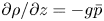 $\partial \rho /\partial z = -g\bar {p}$) where
  $\boldsymbol {u}$ is the velocity,
  $\boldsymbol {g}$ is the gravitational acceleration in the direction of the density gradient,
  $\alpha$ is the thermal diffusivity and
  $\nu$ is the kinematic viscosity
 \begin{gather} \boldsymbol{\nabla}\boldsymbol{\cdot} \boldsymbol{u} = 0; \end{gather}
 \begin{gather}\frac{\partial \boldsymbol{u}}{\partial t} + \boldsymbol{u} \boldsymbol{\cdot}\boldsymbol{\nabla}\boldsymbol{u} ={-}\boldsymbol{\nabla} p' +\nu \cdot \nabla^2 \boldsymbol{u} + \rho'\boldsymbol{g} \end{gather}
 \begin{gather}\frac{\partial \rho '}{\partial t} + \boldsymbol{u} \boldsymbol{\cdot} \boldsymbol{\nabla} \rho ' = w\cdot \frac{\textrm{d} \bar \rho}{\textrm{d} z} + \alpha \cdot \nabla^2 \rho ' . \end{gather}
 Simulations were conducted at  $Re = [200, 300 , 500, 1000]$ and
  $Fr = [0.5, 1, 2, 4, 8]$. Both
  $U$ and
  $R$ are maintained at a constant value of 1 for each simulation, so changes to
  $Fr$ are made by altering
  $\textrm {d}\rho /\textrm {d} z$ and changes to
  $Re$ are made by altering
  $\nu$. In a thermally stratified water column, the ratio of momentum to thermal diffusivity, as measured by the Prandtl number is
  $Pr = \nu/\alpha = 7$. In a salt stratification with molecular diffusivity,
  $D_s$, the equivalent Schmidt number is
  $Sc = \nu/D_s = 700$. The small-scale resolution requirements in the simulations thus rise accordingly, and here we set
  $Pr = 1$. The computations will not be expected to resolve the small scales of scalar gradients. Temporal and spatial derivatives are second-order accurate. Figure 1 shows the computational domain and observation window. The computational domain was
  $16D \times 16D\times 70D$ in the
  $(y,z,x)$ directions respectively. To focus on the near-wake properties, and to avoid possible boundary effects, measurements are only taken up to
  $x/D = 15$. A coarse mesh with 3 M cells was used for
  $Re = (200, 300, 500)$. A finer mesh with approximately 17 M cells is used for
  $Re = 1000$. The mesh is always finer close to the body: the near wake has 1.7 M cells in the coarse mesh and 11.8 M for the fine mesh. In order to reduce reflections from internal waves at the domain boundaries, zero gradient boundary conditions are adopted. The sphere is oscillated back and forth in each direction once to break flow symmetry (Lee Reference Lee2000).

Figure 1. Computational domain for near-wake sphere simulations. Results are taken from a smaller domain outlined in red with dimensions  $4D \times 4D \times 15D$, in the
  $(y,z,x)$ directions respectively.
2.2. Experimental set-up
Experiments were conducted in a  $1\,\textrm {m} \times 1\,\textrm {m}\times 2.5\,\textrm {m}$ tow tank. Stratification and optical access were achieved using a refractive index matched two-tank filling method (Xiang et al. Reference Xiang, Madison, Sellappan and Spedding2015). The sphere was towed from right to left and was suspended from a translation stage with three thin wires of diameter,
  $d = 0.5$ mm as shown in figure 2;
  $Re$ and
  $Fr$ were kept near nominal values of
  $Re = [200, 300, 500, 1000]$ and
  $Fr = [0.5, 1, 2, 4, 8]$, matching the simulations. Each experimental run was performed a minimum of six times.

Figure 2. Experimental set-up for sphere wake experiments. Distances shown are with respect to the largest diameter sphere tested,  $D = 11.1$ cm.
Table 1 shows the experimental parameters for each  $Re$ and
  $Fr$ tested. The kinematic viscosity,
  $\nu = 1.0005 \times 10^{-6}$ m
 $^2$ s
 $^{-1}$. The temperature of the water was maintained near
  $25 \pm 1\,^{\circ }$C. Refractive index matching can cause variations in the kinematic viscosity. For
  $N=0.37$ rad s
 $^{-1}$ the salinity of the water at the bottom of the tank was 35 g NaCl kg
 $^{-1}$ H
 $_2$O. A transition from fresh water to a salinity of 35 g kg
 $^{-1}$ at 25
  $^{\circ }$C corresponds to a
  ${\rm \Delta} \nu /\nu \approx 0.1$ over the height of the fluid (Nayar et al. Reference Nayar, Sharqawy, Banchik and Lienhard2016) for a possible 10 % variation in
  $\nu$. The variations of
  $\nu$ over the diameter of the largest sphere are less than 2 %. Although flow transitions for sphere wakes, both stratified and unstratified, are sensitive to
  $Re$ for
  $Re \leq 1000$, the difference in
  ${\rm \Delta} Re$ from
  ${\rm \Delta} \nu$ did not move the data from one flow regime to another in these tests.
Table 1. Tow speed,  $U$ (cm s
 $^{-1}$), sphere diameter,
  $D$ (cm), and buoyancy frequency,
  $N$ (rad s
 $^{-1}$), for each experimental configuration. The naming convention
  $RxFy$ will be used for
  $Re$ = x00,
  $Fr =y$.

The tank was filled with water/salt/alcohol to a height,  $H = 80$ cm, which ensured the centre of the largest diameter sphere was 3.6
 $D$ away from both the free surface and the bottom of the tank. In this configuration the sphere travelled 10
 $D$ before data acquisition. Data acquisition began when the centre of the sphere was in the middle of the field of view, which was set to a streamwise location to postpone contamination from start and end conditions. The startup transients in the wake propagate upstream, dragged there by the wake itself. When the sphere stops, the wake collides with the sphere, and any bow-wave type conditions bounce off the front wall, and back into the sphere and wake. These effects limit the observation time window available. That time window depends on operating conditions, and is determined from flow visualisation experiments and then checked when practicable by ensuring statistical similarity at different
  $x$ positions within the field of view (FOV).
Two components of velocity were obtained in the horizontal ( $xy$) and vertical (
 $xz$) centreplanes using a planar particle imaging velocimetry system. The tank was filled with titanium dioxide particles with an average density of 4.23 g cm
 $^{-3}$ and diameter of 15
  $\mathrm {\mu }$m. The image plane was illuminated with an Nd:YAG laser operated at a wavelength of 532 nm and a repetition rate of 20 Hz. Images were processed using a multipass algorithm with initial interrogation box size of
  $64 \times 64$ pix with 50 % overlap to a final box size of
  $32 \times 32$ pix. The box resolution therefore ranged from 0.05
 $D$ to 0.22
 $D$ in the horizontal plane.
2.3. Analysis
The averaged results from experiments are ensemble averages over all repeated experimental runs. Wake quantities are averaged with respect to the moving body for each downstream position,  $\boldsymbol {x}$. In a vertical slice, the mean wake quantity can be written
 \begin{equation} \bar{q}(\boldsymbol{x}) = \frac{1}{K}\sum_{i=1}^{K} q_{i}(x, 0, z), \end{equation}
where  $\bar {q}$ is the ensemble-averaged wake quantity at downstream location
  $\boldsymbol {x}$,
  $q_{i}$ is the instantaneous value at
  $\boldsymbol {x} = (x, 0, z)$. Subscript
  $i$ designates the laboratory reference frame of the data. For example
  $q_{1}(c,0)$ is the first instance when wake data were available at downstream location
  $(c,0)$. The parameter
  $K$ is the total number of ensembles for a single run;
  $K = 100$ for the smallest diameter sphere and 54 for the largest. The ensemble averages for each experimental run are then averaged together over all runs. Figure 3 shows an example of three ensembles at downstream location
  $x = 0$ and
  $x=c$ for three laboratory reference frames. The same averaging technique is used in the horizontal plane,
 \begin{equation} \bar{q}(\boldsymbol{x}) = \frac{1}{M}\sum_{i=1}^{M} q_{i}(x, y, 0), \end{equation}
where,  $\bar {q}(\boldsymbol {x})$, is the wake-averaged quantity at coordinates
  $\boldsymbol {x}=(x, y, 0)$, and
  $M$ is the total number of ensembles available in the horizontal plane for position
  $\boldsymbol {x}$. In the horizontal plane
  $M$ varied between 124 and 287 for the largest and smallest sphere cases, respectively. The r.m.s. fluctuating quantities based on temporal averaging in the vertical and horizontal plane are
 \begin{gather} q'(\boldsymbol{x}) = \left[\frac{1}{K}\sum_{i=1}^{K} (q_{i}(\boldsymbol{x}=(x, 0, z))-\overline{q_i}(\boldsymbol{x}))^2\right]^{1/2} \end{gather}
 \begin{gather}q'(\boldsymbol{x}) = \left[\frac{1}{M}\sum_{i=1}^{M} (q_{i}(\boldsymbol{x}=(x, y, 0))-\overline{q_i}(\boldsymbol{x}))^2\right]^{1/2} . \end{gather}
Vertical and horizontal half-wake heights and widths,  $L_v$ and
  $L_h$ respectively, are calculated based on distance from the centreline to the point where the local time-averaged velocity is 15 % of the centreline velocity,
  $\bar {u} = 0.15U_0$ (matching the criteria in Orr et al. Reference Orr, Domaradzki, Spedding and Constantinescu2015) with which we make comparison.

Figure 3. Example of wake quantity,  $q$, ensembles at downstream locations
  $x = 0$ and
  $x=c$ as the sphere moves through the field of view in a fixed laboratory frame of reference;
  $q$ could be a directly estimated quantity, such as
  $\{u, v, w\}$, or a derived measure from spatial derivatives.
The buoyancy frequency,  $N$, has units of rad s
 $^{-1}$, so a buoyancy time scale in seconds is
  $t_b = 2{\rm \pi} /N$. The time required for a neutrally buoyant particle at mid-equator to move on a semi-circle around a sphere of diameter
  $D$ is
  $t_c = {\rm \pi}D/2U$. A maximum resonance between buoyancy-induced internal waves and displacement of fluid over the body occurs when the buoyancy time scale,
  $t_b$, is twice the convective time scale,
  $t_c$. Their ratio is then
 \begin{equation} \frac{t_b}{2t_c} = \frac{2{\rm \pi}}{N}\frac{U}{{\rm \pi} D}=\frac{2U}{ND}, \end{equation}
and a Froude number based on  $D/2$ will equal 1 when
  $t_b=2t_c$.
3. Results
3.1. Wake structure
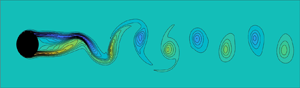
The wake vorticity field will be described from the simulation results, since simulation and experimental results will later be shown to be similar. Figures 4 and 5 show the instantaneous vertical,  $\omega _z$, and lateral,
  $\omega _y$, vorticity in the horizontal and vertical centreplane, respectively, at
  $Re = [200, 500, 1000]$ and
  $Fr = [0.5, 1, 8]$. All snapshots were taken at the same simulation time step
  $t^{*} = Ut/D = 75$.

Figure 4. Vertical vorticity,  $\omega _z(x,y)$ for
  $Re = [200, 500, 1000]$ and
  $Fr = [0.5, 1, 8]$ from simulations. Each plot has 10 evenly spaced contours over
  $\pm {|\omega _z/N|_{max}}$. The reference colour bar in the figure is for
  $F8R10$. Note that the vertical scale in
  $y$ is expanded.

Figure 5. Lateral vorticity,  $\omega _y(x,z)$ for
  $Re = [200, 500, 1000]$ and
  $Fr = [0.5, 1, 8]$ from simulations. Each plot has 10 evenly spaced contours over
  $\pm {|\omega _y/N|_{max}}$.
In figure 4 there are distinct, and different, variations in the wake geometry for variations in both  $Re$ and
  $Fr$. The middle column, for
  $Fr = 1$, varies the least with
  $Re$. At this maximum resonance condition ((2.10),
  $t_b=2t_c$) the lee waves control the conditions on the sphere and the wake is symmetric, at all
  $Re$, in both horizontal and vertical centreplanes (figure 5, centre column). As the stratification is relaxed (
 $Fr = 8$, right column), the centreline symmetry is maintained in both horizontal and vertical planes at low
  $Re = 200$, but is broken for
  $Re \geq 500$ (cases
  $R5, R10$ in the rightmost
  $F8$ column). In
  $F8R10$ there are strong gradients in both
  $\omega _z$ and
  $\omega _y$, and evidence of a number of smaller scales of motion behind the sphere and in the developing wake.
When  $Fr = 1$, the flow in the vertical centreplane travels around the sphere edge, rejoining almost at the equatorial plane. The dominant wavelength in the streamwise direction does not vary with
  $Re$ (middle column, figure 5). In the left column of figures 4 and 5,
  $t_b \approx t_c$ and the preferred internal wavelength is shorter than a half-circumference, so the flow departs from the sphere at an azimuth angle of approximately
  $2{\rm \pi} /3$. In the horizontal centreplane, the shear layers extend further downstream as the flow is forced to travel around the sphere, rather than above and below it. At all
  $Re$, the wake now destabilises in the horizontal, with high amplitude (
 $\xi > R$) excursions. The wavelength decreases with increasing
  $Re$. Pal et al. (Reference Pal, Sarkar, Posa and Balaras2016) and Chongsiripinyo et al. (Reference Chongsiripinyo, Pal and Sarkar2017) also found a rebirth of turbulent fluctuations with decreasing
  $Fr$ below 0.5 (at fixed
  $Re = 3700$), and although
  $Re$ here is insufficient to produce turbulence, the strong gradients in
  $\omega _z$ and in
  $\omega _y$ for
  $F.5R10$ (bottom left corner of figures 4 and 5) show the same, and somewhat counter-intuitive, consequence of the quasi-2-D forcing.
The qualitatively different wakes in figures 4 and 5 are placed in a { $Re$–
$Re$– $Fr$} diagram and compared with the observations from CH93 in figure 6. A classification of the wakes from both experiment and simulation is shown by coloured symbols. For
  $Fr \leq 1$, variations in
  $Re$ were not important and the wakes transition from steady, planar symmetric (red) to unsteady vortex shedding (purple) as
  $Fr$ decreases from 1. The regimes from CH93 are saturated lee wave, and two-dimensional, the latter since the centreplane and nearby layers generate vortex wakes much as a 2-D cylinder would. For
  $Fr = 2,4$ the CH93 classification was of a transitional regime (T) without, and then with Kelvin–Helmholtz (KH) instability with increasing
  $Fr$. In the current study, there is a variation with
  $Re$ at these intermediate
  $Fr$, and the wakes at
  $Fr = 2$ can be planar symmetric (red), vertically asymmetric but horizontally symmetric (yellow) or planar oscillating (green, the equivalent of KH in T). The planar oscillation is seen at higher
  $Fr$, lower
  $Re$ also, in regions that lie outside the experiments of CH93. Multiple unsteady modes appear at higher
  $Fr$ (blue), at lower
  $Fr$ for higher
  $Re$. The detailed studies of LI92 and CH93 paid close attention to conditions on the sphere, especially at low {
 $Re$,
$Re$,  $Fr$}. Here, we are mostly concerned with the pattern and geometry in the intermediate wake (omitting details of recirculation and separation zones) that then may, or may not persist into later times. In this respect, we note that the wake decay at large
  $x$ could be enhanced in figures 4, 5 through numerical diffusion in the low-order method. The regimes identified are qualitatively consistent with existing literature, and the flow fields and their parametric variations can now be examined quantitatively

Figure 6. The { $Re$,
$Re$,  $Fr$} regime diagram for the current experiments (coloured shapes) and from CH93 (background). CH93 divided the space mainly by
  $Fr$ into four main subregions: two-dimensional, saturated lee wave (SLW), transition (T) and three-dimensional (3-D). The vertical dashed lines bound each subregion in
  $Fr$,
$Fr$,  $Re$ space. The symbols denote wake structure across
  $Fr$,
$Fr$,  $Re$ for the present study: horizontal vortex street (purple circles), steady, planar symmetric (red squares), vertical asymmetric (yellow triangle), planar oscillation (green diamonds) and multiple unsteady modes (blue right facing triangle).
3.2. Time-averaged wake properties
3.2.1. Streamwise velocity comparison
Figure 7(a,c,e,g) shows the time-averaged streamwise velocity,  $\bar {u}/U$, for simulations and experiments (b,d,f,h) in the vertical centreplane for constant
  $Fr = 1$ and varying
  $Re$. The most prominent feature at
  $Fr = 1$ is the lee wave which causes an initial decrease in wake height just behind the sphere. The amplitude of the contraction increases with increasing
  $Re$. The contraction occurs with a local minimum in the streamwise centreline velocity and has been observed at
  $Re > 1000$ for spheres (Bonnier & Eiff Reference Bonnier and Eiff2002; Pal et al. Reference Pal, Sarkar, Posa and Balaras2017) and behind towed grids (Xiang et al. Reference Xiang, Madison, Sellappan and Spedding2015). The minimum
  $\bar {u}$ occurs at
  $x/D = 1.5$ for all
  $Re$ simulations and at
  $x/D = 1.3 \pm 0.1$ for the experiments. The spacing and amplitude of the wake pulsations is unaffected by
  $Re$. The background level in experiments is lower (darker) because very small pixel displacements are on average drawn back to 0 due to peak locking.

Figure 7. Time-averaged streamwise velocity,  $\bar {u}/U(x,z)$ for
  $Fr = 1$ and
  $Re=[200, 300, 500, 1000]$. Simulations are in (a,c,e,g), laboratory experiments are in (b,d,f,h). Each case has 10 evenly spaced contours between
  $\bar {u}_{max}$ and
  $\bar {u}_{min}$.
Figure 8 shows a similar comparison at fixed  $Re = 500$ and varying
  $Fr$. As
  $Fr$ increases, so does the wavelength,
  $\lambda$, of the lee waves;
  $x/D$ can be related to a buoyancy time,
  $Nt$ through
  $x/D = Nt Fr/2$, and the minimum in
  $\bar {u}$ occurs at
  $Nt = 3.3 \pm 0.3$ and
  $Nt = 3.2 \pm 0.3$ for simulations and experiments, respectively at
  $Fr = [1,2,4]$. At
  $Fr = 8$, the minimum would be expected at
  $x/D = 25$, which is outside the observation windows in figure 8. The location of
  $\bar {u}_{min}$ agrees with towed grid experiments where
  $\bar {u}_{min}$ was found between
  $3 \leq Nt \leq 4$ for
  $2700 \leq Re \leq 11000$ and
  $0.6 \leq Fr \leq 9$. The wavelength
  $\lambda$ is expected to be a linear function of
  $Fr$,
$Fr$,  $\lambda = {\rm \pi}Fr$ as verified later.

Figure 8. Time-averaged streamwise velocity,  $\bar {u}/U(x,z)$ for
  $Re =500$ and
  $Fr=[1,2,4,8]$. Conventions are same as in figure 7.
3.2.2. Mean velocity profiles
Figure 9 shows the mean streamwise velocity profiles at several downstream locations rescaled by the local centreline value,  $\bar {u}/U_0$, in both the vertical and horizontal centreplanes for
  $Re = 1000$,
  $Fr = 8$. The vertical and horizontal coordinates are normalised by the local half-height and width,
  $L_v$ and
  $L_h$, respectively. In the vertical centreplane there is good agreement between the simulations and experiments, although for positive values of
  $z/L_v$ the profiles from experiments do not fall to zero. The defect is caused by the wakes of the tow wires, which otherwise appear to be superimposed upon the mean wake with no other effect. The mean wake profile shapes are not otherwise distinguishably different from each other, over
  $x/D = [4 - 15]$.

Figure 9. Rescaled streamwise velocity in the vertical (a) and horizontal (b) centreplanes for  $Re = 1000$ and
  $Fr = 8$. Black and red lines correspond to simulations and experiments, respectively.
Initially the horizontal plane velocity profiles in figure 9(b), are more varied, and the peak values of  $\bar {u}/U_0$ may be off centreline, as also found in OR15 for
  $Re = 1000,\ Fr \geq 4$. The horizontal profiles reach a similar state by the end of the simulation domain. For this particular case
  $x/D = 8$ corresponds to
  $Nt = 2$, when buoyancy effects are thought to become significant, and vertical and horizontal profiles, although similar, are not the same.
Figure 10 shows rescaled velocity profiles from experiment further downstream at  $x/D = [15, 20, 25, 30]$ for the horizontal and vertical centreplanes. Profiles in the vertical plane retain their shape even at
  $x/D = 30$. At the furthest
  $x/D$ observed the horizontal plane profiles have a similar shape to the velocity profiles in the vertical plane. The similar profile shapes encourage a search for regularities that govern the time evolution of length and velocity scales.

Figure 10. Rescaled streamwise velocity profiles farther downstream in measurements from horizontal and vertical centreplane experiments for  $Re = 1000$ and
  $Fr = 8$.
3.2.3. Wake length scales
Figure 11 shows the variation in vertical length scales with  $Re$ and
  $Fr$, and for experiment and simulation. The agreement between experiment and simulation is satisfactory, as the amplitudes and wavelengths together with variations in governing parameters are the same. At the lowest
  $Fr = 1$, local wake heights are strongly shaped by lee waves initiated at the body. For each {
 $Re$,
$Re$,  $Fr$} pair, the internal wave oscillation is superimposed on a gradual growth in
  $L_v$. At lower
  $Re$,
$Re$,  $L_v$ almost doubles over
  $x/D \approx 15$. Higher
  $Re$ wakes have smaller
  $L_v$ and they grow less rapidly in
  $x$, as seen qualitatively in figure 7. At higher
  $Re$, kinetic energy can be driven towards small-scale mixing, rather than slow laminar growth in an internal-wave-dominated near field. The vertical growth is strongly limited by the background stratification when everywhere
  $Fr \leq 1$.

Figure 11. Downstream evolution of  ${L_v}/{R}$ for simulations (black lines) and experiments (red lines); (a)
  $F1$, (b)
  $F2$, (c)
  $F4$, (d)
  $F8$.
$F8$.
As  $Fr$ increases, the wavelength and amplitude of the wake disturbances increase. At
  $Fr = 8$ the
  $Re$ trend abruptly reverses as now higher
  $Re$ leads to higher
  $L_v$. At
  $Re = 1000$,
  $L_v$ increases at first, and then stays almost constant. This region of constant
  $L_v$ was found by Spedding (Reference Spedding2002) where the first available measurements were at
  $x/D = 10$. This almost constant
  $L_v(x/D)$, even decreasing slightly at first, can also be seen in Diamessis et al. (Reference Diamessis, Spedding and Domaradzki2011), where the initial height increases with
  $Re$, and in Dommermuth et al. (Reference Dommermuth, Rottman, Innis and Novikov2002), Brucker & Sarkar (Reference Brucker and Sarkar2010) and Zhou & Diamessis (Reference Zhou and Diamessis2019). Reports of
  $L_v(x)$ vary considerably in detail in the literature (ops cit.), with variations from both
  $Fr$ and
  $Re$. Differing physical mechanisms could be behind similar
  $L_v$ observations, and Meunier, Diamessis & Spedding (Reference Meunier, Diamessis and Spedding2006), for example, contend that the low-growth region is only a consequence of the slow transition between turbulent and viscous scaling regimes.
It has been noted before (Spedding, Browand & Fincham Reference Spedding, Browand and Fincham1996b) that a lower limit on  $Fr$ that allows turbulence over some range of scales can be estimated through the Ozmidov scale,
  $l_0$, the largest overturning scale allowed by the stratified ambient
 \begin{equation} l_0 \sim \left(\frac{\epsilon}{N^3}\right)^{1/2}, \end{equation}
where  $\epsilon$ is the kinetic energy dissipation rate. In homogeneous turbulence
  $\epsilon \sim u'^3/l$, where
  $u'$ is a fluctuating velocity and
  $l$ an integral length scale so
 \begin{equation} l_0 \sim \left(\frac{u'^3}{lN^3}\right)^{{1}/{2}}. \end{equation}
For turbulent scales of  $l$ to be initially unaffected by the stratification,
  $l_0 \geq l$ and
 \begin{equation} \left(\frac{l_0}{l}\right) = \left(\frac{u'}{U}\right)^{{3}/{2}} \left(\frac{l}{D}\right)^{-({3}/{2})} \left(\frac{U}{ND}\right)^{{3}/{2}} \geq 1. \end{equation}
In unstratified sphere wakes (Gibson, Chen & Lin Reference Gibson, Chen and Lin1968; Uberoi & Freymuth Reference Uberoi and Freymuth1970),  $u'/U \approx 0.3$ and
  $l/D \approx 0.4$ so
 \begin{equation} \left(\frac{U}{ND} \right)^{{3}/{2}} \geq 5,\quad Fr \geq 3. \end{equation}
These arguments are concerned with when a minimum range of length scales for turbulent energetics could be expected, hence when the turbulent dynamics may explain wake length scales. Here, the { $Re$–
$Re$– $Fr$} range covers a region mostly in laminar and stratification-dominated wakes, and the strong influence of the body-generated lee wave can be seen throughout figure 11. Figure 12 shows the first minimum half wake height
  $(L_v/D)_{min}$ as a function of
  $Fr$ for all the simulations. When
  $Fr < 4$,
  $(L_v/D)_{min}$ decreases as
  $Re$ increases. For
  $Fr \geq 4$ the vertical scales can be influenced by the first signs of turbulence, and the differences in
  $(L_v/D)_{min}$ with
  $Re$ begin to shrink. Computations at higher
  $Re \in [1, 4 \times 10^5]$ (Zhou & Diamessis Reference Zhou and Diamessis2019) show that
  $Fr$ is less influential in determining vertical scales as
  $Re$ increases, perhaps because the evolving flow has spent longer at
  $\mathcal {R} > 1$.

Figure 12. Vertical wake half-height,  $(L_v/D)_{min}$ for simulations as a function of
  $Fr$.
$Fr$.  $Re$ are given by the symbols in the legend.
The mean wake height (minus lee-wave-induced oscillations) increases with downstream distance, and given the similar forms of the velocity profiles found in figures 9 and 10 we may find a power law of the form  $L_v/D \approx \alpha (x/D)^\beta$. Table 2 shows the fitting coefficients,
  $\alpha$ and
  $\beta$, for the simulations and experiments. The average growth rate,
  $\beta$, for the simulations is
  $0.29 \pm.05$ and for the experiments is
  $0.27 \pm.06$. These wake growth rates do not show a clear dependence on either
  $Fr$ or
  $Re$. They have been measured at
  $x/D$ much smaller than previous experimental vertical stratified wake data (Spedding Reference Spedding2002). Pal et al. (Reference Pal, Sarkar, Posa and Balaras2017) have measured
  $L_v$ in a sphere-inclusive simulation but did not attempt a parametrisation. Chongsiripinyo et al. (Reference Chongsiripinyo, Pal and Sarkar2017) have given detailed descriptions of the vortex dynamics and structures, focusing on
  $Fr < 1$, pointing out that the near-wake structures would be essential in carrying information from the near wake into the later stages of development.
Table 2. Power law coefficients for wake height,  $L_v$, for all
  $Re$ and
  $Fr$ found from simulation results;
  $\alpha _e$ and
  $\beta _e$ are coefficients for the experiments.

It is clear that vertical length scales in the stratified wake can show significant variation with both  $Re$ and
  $Fr$, and that the relative importance of turbulent motions then also delineates regimes where
  $\mathcal {R}$ is large or small. Furthermore, it is also likely, given the different literature findings, that initial conditions play an as-yet unexamined role. We shall return to this topic in the discussion section.
The lee wavelength,  $\lambda$, was determined from the streamwise distance between extrema in
  $x$ of the half-wake height. Figure 13 shows the normalised lee wavelength as a function of
  $Fr$ for the
  $R10$ simulations and experiments. In a linear density gradient, the natural cyclic buoyancy frequency is
  $N/2{\rm \pi}$, and the wavelength is then
  $\lambda = 2{\rm \pi} U/N$ or
  $\lambda /D = {\rm \pi}Fr$, independent of
  $Re$. This relationship accounts well for the observations from experiment and simulation, and from measurements from Meunier et al. (Reference Meunier, Le Dizes, Redekopp and Spedding2018) for
  $Fr \leq 2$. When
  $Fr > 2$, the experiments, simulations and Meunier et al. (Reference Meunier, Le Dizes, Redekopp and Spedding2018) still agree but are slightly larger than the values predicted by linear theory.

Figure 13. Wake wavelength,  $\lambda /D$ vs
  $Fr$ for
  $R10$ simulations, experiments and from Meunier et al. (Reference Meunier, Le Dizes, Redekopp and Spedding2018).
Figure 14 shows the downstream evolution of the half-wake width,  $L_h/R$. The
  $L_h(x)$ curves are qualitatively different, depending on
  $Fr$. At low
  $Fr \leq 4$ the same footprint of lee waves as seen in figure 11 occurs in
  $L_h$ (cf. figures 7 and 8). Only when
  $Fr = 8$ do the curves show a more gradual increase. There are significant differences between experiment and computations over the intermediate ranges
  $Fr = 2,4$ and
  $Re = 500, 1000$. The
  $F2R10$ case has been re-run and investigated closely, and the differences remain. The
  $L_h$ measure is affected by the unsteadiness in the simulation, which is not present in experiment, or in the simulations of OR15. The unsteady solution appears to be affected by the startup conditions where the sphere is accelerated back and forth, sending this borderline case to the KH regime rather than a regime without KH modes (SKH). The
  $F8R5$ curves differ because the grid resolution was too low as the emerging turbulence generates smaller scales. In general, the solutions for experiment and simulation match closely.

Figure 14. Wake width,  ${L_h}/{R}$ from experiment and simulation for
  $Fr = 1, 2, 4, 8$ in (a–d). Simulations are in black, experiments in red.
3.2.4. Centreline velocity
Figure 15 shows the mean centreline velocity evolution,  $(U_0/U)$ vs
  $(x/D)$ for various
  $Re$ and
  $Fr$ combinations in simulation and experiment. At the lower
  $Re$ (figure 15a) and lower
  $Fr$ (figure 15c), there is no strong dependence on either
  $Fr$ or
  $Re$. At
  $Fr = 1$ (figure 15c), the lee waves are the dominant influence, and
  $U_0$ cycles up and down out of phase with the product of
  $L_h L_v$, as required for continuity. These fluctuations at lower
  $Re$,
$Re$,  $Fr$ have been referred to as wake collapse (cf. Bonnier & Eiff Reference Bonnier and Eiff2002; Xiang et al. Reference Xiang, Madison, Sellappan and Spedding2015) although nothing is collapsing (figures 11 and 14) and the oscillatory function lies on top of a gradual and uniform decay. At higher
  $Re$ and higher
  $Fr$ there is a single rise in
  $U_0$ and then a decay with
  $x/D$ that is more pronounced at higher
  $Fr$ and
  $Re$, respectively.

Figure 15. Downstream evolution of the normalised mean centreline velocity,  $U_0/U$ for (a)
  $Re = 200$, (b)
  $Re = 500$, (c)
  $Fr = 1$, (d)
  $Fr = 8$. Simulations in black, experiments in red.
There is good agreement between experiment and simulation for  $U_0(x)$, better than for the
  $L_h$ measure, supporting the idea that the physics computed and measured are the same, but some averaging processes are less robust in limited averaging domains.
Early work on stratified sphere wakes had no means of reliably measuring wake characteristics at early times because the apparatus could not readily deploy refractive index matching, and the earliest measurement times were at  $Nt \approx 10$. From these times onward, it was notable, and curious, that the mean and turbulence quantities then seemed to evolve according to power laws which could be written in terms as though the influence of stratification (through
  $Fr$) were negligible. Then, since
  $x = Ut$, we can make the equivalence
  $x/D = (Nt)Fr/2$ and expressions of the form
 \begin{equation} \left.\begin{gathered} \frac{U_0}{U} = \alpha \left(\frac{x}{D}\right)^\beta \\ \frac{U_0}{U}Fr^{-\beta} = \alpha \left(Nt\right)^\beta \end{gathered}\right\}, \end{equation}
can be written. The exponent  $\beta$ does not change between the two forms, and the only difference is the position in
  $x/D$ or
  $Nt$ for the data, which depends on
  $Fr$. In stratified flows that decay and eventually come under the leading influence of buoyancy, one might expect
  $Fr$-independent, 3-D dynamics first and then when buoyancy enters, it may do so at some fixed
  $Nt$. Instead,
  $Fr$-independent power laws were measured even at late times. The
  $Fr$-independence in strongly stratified turbulence was explained and predicted by Billant & Chomaz (Reference Billant and Chomaz2001), when
  $l_v = U/N$. Here, we are interested in when the initial early wake transitions into NEQ and Q2D states, so it is useful to plot a rescaled
  $U_0 (Nt)$.
Figure 16 shows the evolution in  $Nt$ of the centreline velocity for
  $Re = 300, 1000$ with varying
  $Fr$. Here, the wake defect is just emerging into the
  $Nt$ domain (
 $Nt \approx 3$) where previous experiments made their first measurements (Spedding Reference Spedding2001). The data do not show a low decay rate that has classically described the NEQ regime, but at low and high
  $Re$ emerge at approximately
  $Nt = 10$ with a decay law that is similar to
  $-2/3$ (
 $-0.66 \pm 0.14$ and
  $-0.63 \pm 0.11$) for simulation and experiment, respectively. Spedding, Browand & Fincham (Reference Spedding, Browand and Fincham1996a) found NEQ–Q2D scaling only for
  $Re \geq 4000$, so the rather moderate success in collapsing
  $U_0$ at
  $Re = 1000$ is not in conflict. If the early signs of
  $-2/3$ decay are correct, then, if applicable, they must describe a regime that precedes the previously measured wakes. Although the decay rates are the same as for a turbulent, unstratified wake, the non-negligible influence of the stratification has been evident in all the preceding data.

Figure 16. Rescaled centreline velocity,  $(U_0/U)Fr^{-2/3}$ for (a)
  $Re = 300$ and (b)
  $Re = 1000$ vs buoyancy time scale,
  $Nt$, for
  $Fr = 1,2,4,8$. Solid, dash, dash-dot and dotted lines correspond to
  $Fr = 8,4,2,1$, respectively.
3.3. Fluctuating velocities and the buoyancy Reynolds number
The maximum  $Re$ here, based on the sphere diameter and tow speed, is 1000, and the flow can hardly be considered turbulent. However, all decaying wakes, globally, or locally, will eventually enter a stage in which
  $Re$ is small, so there is some interest in what fluctuating quantities look like even at small
  $Re$. Then the questions arise as to how this state was achieved and whether the origin from a higher energy state is relevant.
In this experiment, fluctuating quantities as defined in (2.8) and (2.9) can come from two sources: one is from unsteady activity in the wake at large scales, where coherent structures pass through measurement points, or volumes. The second is from fluctuations that derive from the turbulent dynamics. Referring to figures 4 and 5, only the lower right corner could qualitatively be described as turbulent, although it is easy to see how non-negligible fluctuations will occur in other situations, such as for  $Fr = 0.5$. The measurements of
  $u', v', w'$ described here are therefore not measures of turbulence, but are diagnostic measures of these early wakes in their various {
 $Re$–
$Re$– $Fr$} states.
Figure 17 compares { $u', v', w'$} at three downstream locations,
  $x/D = [3, 5, 10]$ for
  $Re = 1000$ and
  $Fr = 8$. At each downstream location the simulations and experiments agree well. The magnitude of the peaks of the streamwise fluctuations decreases with downstream distance while the width of the peaks increases as the wake width increases.
  $u'(y)$ has a double-peaked profile, as would be obtained when fluctuating quantities are associated with mean shear.
  $v'(y)$ has a similar shape although with smaller-amplitude peaks.
  $w'(z)$ has only a single maximum, which decays faster with
  $x/D$ than the horizontal components. The first turbulence profiles for a stratified wake (Spedding Reference Spedding2001) were measured at
  $x/D = 6$ (or
  $Nt = 9$) and all three fluctuating velocity components were initially double peaked. The difference comes from
  $Re$, which was 5000 in the previous study, and 1000 here.

Figure 17. Fluctuating velocity components (a)  $u'(y)$, (b)
  $v'(y)$ and (c)
  $w'(z)$ for
  $Re = 1000$,
  $Fr = 8$. Simulations and laboratory experiments are represented by solid and dashed lines, respectively.
The dependence of the velocity fluctuation magnitudes on  $Re$ and
  $Fr$ is shown in figure 18. At
  $Re = 300$
  $w'_0$ falls almost immediately to approximately 1 % of
  $u'_0$, for all
  $Fr$. At
  ${\rm Re} = 1000$ the
  $Fr = 4, 8$ cases remain at
  $w'_0/u'_0 \approx 1$ up to
  $x/D = 15$. There are fluctuations in the ratio with wavelength equal to the lee wavelengths. The averages are temporal averages so the lee waves themselves, which are steady in the sphere reference frame, do not directly contribute to
  $w'_0$, but some components of this wave-induced field clearly impact the measurement. In this respect then, all wakes are buoyancy influenced at all times.

Figure 18. Ratio of centreline fluctuations  ${w_0' }/{u_0'}$ for (a)
  $Re = 300$ and (b)
  $Re = 1000$ for varying
  $Fr$, as given in legend of (a).
It is useful to locate the sphere wakes discussed here in  $Fr_h-\mathcal {G}$ space described by de Bruyn Kops & Riley (Reference de Bruyn Kops and Riley2019). The wake properties are not uniform so we make local measures as explored and detailed in Xiang et al. (Reference Xiang, Madison, Sellappan and Spedding2015) and Zhou & Diamessis (Reference Zhou and Diamessis2019). The latter authors proposed a criterion of
  $ReFr^{-2/3} \geq 5 \times 10^3$, based on initial wake parameters,
  $D$ and
  $U$, could be used to indicate activity in a strongly stratified regime ((1.2) and after). At the highest {
 $Re$,
$Re$,  $Fr$} combination here
  $ReFr^{-2/3} = 250$, far below the suggested criterion. The relationship is counter-intuitive, however, as the product
  $ReFr^{-2/3}$ decreases for increasing
  $Fr$ and fixed
  $Re$. Thus for
  $Fr = 1$, the product is 1000, while for
  $Fr = 32$, it is 100. This is because the quantity
  $\mathcal {G}$ aims to give relations when stratification is strongly felt, yet
  $Re$ is still high, and blindly following this prescription would indicate that the
  $R10F1$ case is closer to SST than is
  $R10F8$. This cautionary note notwithstanding, we may make some local calculations, close to the wake edge, in order to estimate both
  $\mathcal {G}$ and
  $Fr_h$. The reasoning follows the arguments of Billant & Chomaz (Reference Billant and Chomaz2001) who show that there is a limit where a strongly stratified flow adjusts so that
  $Fr_v = 1$, when
  $l_v = U/N$. The length scale evolution is then indicated by
  $Fr_h = u'/Nl_h$, where
  $l_h$ is the local horizontal length scale. This measure is derived from autocorrelations of time series of
  $w'$. The autocorrelation is plotted vs the lag number and the distance to the first zero crossing of the autocorrelation function is multiplied by the time interval, expressed as
  $t_{loc}$. Then the associated local horizontal length scale,
  $l_h = u't_{loc}$. The process is similar to that used by Diamessis, Gurka & Liberzon (Reference Diamessis, Gurka and Liberzon2010) and Xiang et al. (Reference Xiang, Madison, Sellappan and Spedding2015), and is repeated for each experimental run and then averaged over all runs. If we retain the local
  $u'$ as a measure of the available kinetic energy in velocity fluctuations, and we keep
  $l_h$ as an indicator of turbulent length scales, then
 \begin{equation} \left.\begin{gathered} Fr_t = \frac{u'}{Nl_h} \\ Re_t = \frac{u'l_h}{\nu}, \end{gathered}\right\} \end{equation}
and  $\mathcal {G}$ can be calculated from (1.2) without direct recourse to assumptions about the isotropy of
  $\epsilon$, for example. We may note that variations in
  $\rho$ and its gradient
  $\partial \rho /\partial z$ are neglected, and a truly local measure may take these into account, however, again, these are approximate indicators of a state which in detail requires the Navier–Stokes equations. Estimates of
  $\mathcal {G}$ and
  $Fr_h$ are plotted in figure 19. The highest value of
  $\mathcal {G}$, for R10F8, is less than 30. Although the condition
  $\mathcal {G} > 1$ is met, recall that
  $\mathcal {G}$ represents the range of scales between an Ozmidov scale
  $l_O$ and a Kolmogorov scale,
  $l_K$, and their ratio,
  $l_O/l_K \sim \mathcal {G}^{4/3}$ (de Bruyn Kops & Riley Reference de Bruyn Kops and Riley2019). The small range of scales implied by
  $\mathcal {G} \leq 30$ is not sufficient for turbulent dynamics to exist or be sustainable. Two lower
  $Fr$ cases are also plotted for the earliest
  $Nt$ available, and even ignoring the dubious calculation assumptions at these low {
 $Re$–
$Re$– $Fr$}, the data lie firmly in the viscous-dominated regime, as they ought. Chongsiripinyo & Sarkar (Reference Chongsiripinyo and Sarkar2020) constructed a similar plot, albeit for a disk wake, and with
  $\mathcal {R}$ on the abscissa. The initial condition of
  $Re = 5 \times 10^4$ allowed a starting point in weak buoyancy effects which then transitioned through all stages, WST–IST–SST, before significant viscous damping.

Figure 19. Plot Regime diagram,  $Fr_h$ vs
  $\mathcal {G}$ for
  $R10$ wakes. The
  $F1$ and
  $F2$ wakes immediately start in the viscous dissipation regime.
4. Discussion and conclusions
This work presents the first quantitative and systematic study through independent variations of  $Re$ and
  $Fr$ of the canonical stratified sphere wake problem. It focuses on the domain of moderate values of both parameters (
 $Re \in [200, 1000]$,
  $Fr \in [0.5, 8]$) where the competing influences of inertial, buoyancy and viscous terms result in a number of qualitatively different flow regimes. The {
 $Re$–
$Re$– $Fr$} parameter space is covered equally for experiments and simulations. By design it also overlaps with certain cases in OR15, and the
  $R10F1$ comparisons are shown in figure 20(a). When
  $Fr = 1$, the lee waves have their strongest influence on the near wake, and there is reasonable agreement up to
  $x/D = 5$. After that, the OR15 values are greater. Figure 20(b), for
  $R10F4$, shows that the differences may be caused at least in part by numerical resolution, as the higher resolution results agree much more closely at large
  $x/D$. Figure 20(a) also includes the equivalent result from Pal et al. (Reference Pal, Sarkar, Posa and Balaras2017) which comes from a significantly higher
  $Re$ run.

Figure 20. Vertical length scale for (a)  $R10F1$ simulations, OR15 and Pal et al. (Reference Pal, Sarkar, Posa and Balaras2017) and (b)
  $R10F4$, OR15 low and high resolutions. Experiments excluded for clarity, as they have been shown to be similar to simulations in the present study.
The reasonable agreements between experiment and simulation here are not completely trivial, since the early wake length and velocity scales depend on details of the separation location. Nevertheless, we would not advocate pushing these second-order methods to higher  $Re$, as significantly more sophisticated numerical methods are required (e.g. Pal et al. Reference Pal, Sarkar, Posa and Balaras2017; de Bruyn Kops & Riley Reference de Bruyn Kops and Riley2019; Zhou & Diamessis Reference Zhou and Diamessis2019) to deal with complex boundaries and/or initial high
  $Re$ turbulence over a range of scales. One should also note that extension to lower
  $Fr$ also requires significant resolution to resolve the fine structures that re-emerge when
  $Fr < 0.5$ (Pal et al. Reference Pal, Sarkar, Posa and Balaras2016; Chongsiripinyo et al. Reference Chongsiripinyo, Pal and Sarkar2017), the lowest
  $Fr$ covered here. Both simulations and experiments will aim to explore higher
  $Re$ domains, and existing work on the importance of the activity parameter denoted here
  $\mathcal {G}$ will be helpful in understanding the location in turbulence–buoyancy interactions.
Funding
This work was supported under grants N00014-15-1-2506 and N00014-20-12548 under program managers Dr R. Joslin, Dr T. Fu and Dr P. Chang. We are most grateful for this.
Declaration of interests
The authors report no conflict of interest.
Appendix A. Checking the numerical simulations
Early experiments and simulations have investigated the unstratified wake behind a sphere for  $Re \leq 1000$ (e.g. Achenbach Reference Achenbach1974; Tomboulides & Orszag Reference Tomboulides and Orszag2000), and results from current simulations are compared in figures 21 and 22.

Figure 21. Streamline projections onto horizontal (a,c,e,g) and vertical (b,d,f,h) planes for the unstratified flow past a sphere.

Figure 22. Estimates of drag coefficient and Strouhal number for unstratified sphere wakes.
The streamlines are shown in figure 21 for unstratified flow in simulations. The wake at  $Re = 200$ is axisymmetric, and has a recirculation region of length
  $1.4D$. At
  $Re = 300$, with weak initial perturbation, the wake cannot maintain axisymmetry, but oscillates at
  $St = fD/U = 0.133$ in one plane, where
  $f$ is the oscillating frequency, while keeping planar symmetry in the other plane. The plane in which the wake oscillates depends on the initial perturbation. The spiral mode forms at
  $Re = 500$ and, in a convective time window of 250, a dual-frequency oscillation at
  $St = 0.168$ and
  $St = 0.044$ is recorded. The wake becomes more irregular at
  $Re = 1000$. A lower frequency is found at
  $St = 0.191$, and another higher frequency around 0.33, but of lower amplitude than the lower-frequency peak. The structural transitions as a function of
  $Re$ were analysed in some detail in Tomboulides & Orszag (Reference Tomboulides and Orszag2000), and the symmetry breaking sequence in figure 21 is in agreement. The steady and unsteady separation sequence leads to variations in
  $C_D$ and
  $St$, which are compared with literature values in figure 22. The agreement is satisfactory for the integrated force measure of
  $C_D$ and for
  $St$, including the simultaneous presence of high and low modes.
Finite volume methods yield numerically induced wave dispersion errors (cf. Fletcher Reference Fletcher1991) where wave propagation angles and speeds vary with frequency/wavenumber. The magnitude of these errors depends on the wavelength,  $\lambda$, in the flow compared with the mesh size,
  $\varDelta$, and can be estimated both a priori and a posteriori for certain configurations (including multidimensional, nonlinear flows) (Schranner et al. Reference Schranner, Domaradzki, Hickel and Adams2015; Castiglioni, Sun & Domaradzki Reference Castiglioni, Sun and Domaradzki2019) but accurate estimates are difficult for 3-D flows on unstructured meshes, and one strives for large
  $\lambda /\varDelta$, The internal waves that we may claim to simulate have
  $\lambda = O(D)$, and dispersion errors will be small when
  $\lambda /\varDelta \approx 0.025$. Internal waves propagate from their source and then the selection of appropriate far-field boundary conditions also becomes more critical. The selection of boundary conditions for the finite volume solvers in OpenFOAM is described in some detail in Chen & Spedding (Reference Chen and Spedding2017), which also describes the generation of the expected St Andrew's cross internal waves in response to periodic pointwise forcing in the domain centre. For
  $\omega /N = \sqrt {3}/2, \sqrt {2}/2$ and 1/2, the angle of the isophase lines from the vertical,
  $\theta$, were not significantly different from predicted values (Lighthill Reference Lighthill1978; Voisin Reference Voisin1991) of
  $\theta = {\rm \pi}/6, {\rm \pi}/4$ and
  ${\rm \pi} /3$.
At low  $Fr$, the near wake is strongly influenced by the lee wave of the sphere and denoting
 \begin{equation} \overline{{\rm \Delta} C_D} = C_D(Re, Fr) - C_D(Re, \infty) \end{equation}
the difference in drag coefficient for varying  $Fr$ is plotted in figure 23(a). In the range
  $0.5 \leq Fr \leq 8$ there is reasonable agreement between experiment and simulations (these and from Rottman et al. Reference Rottman, Brucker, Dommermuth and Broutman2010; Orr et al. Reference Orr, Domaradzki, Spedding and Constantinescu2015). Below
  $Fr = 0.5$ there is considerable variation and Pal et al. (Reference Pal, Sarkar, Posa and Balaras2016) have shown how small-scale fluctuations re-appear at very low
  $Fr$, requiring once again very fine grid resolution.

Figure 23. (a) The change in time-averaged drag coefficient at varying  $Fr$ for a range of experiments and simulations (modified from Orr et al. Reference Orr, Domaradzki, Spedding and Constantinescu2015); (b) lee wavelengths immediately behind the sphere closely match the
  $\lambda = 2{\rm \pi} R.Fr$ prediction.
The wavelength,  $\lambda /2R$ of linear internal waves is
  ${\rm \pi}.Fr$, and matches well with observations here and in the literature, both for spheres (Hanazaki Reference Hanazaki1988; Chomaz et al. Reference Chomaz, Bonetton, Butet and Hopfinger1993) and even quite well for circular cross-section grids (Xiang et al. Reference Xiang, Madison, Sellappan and Spedding2015). At
  $Fr \geq 1$, Voisin (Reference Voisin2007) invokes
  $U/N$ as a scale for outer regions influenced by low-amplitude oscillations in the inner wake and from table 1, for case R10F8,
  $U/(2{\rm \pi} N) \approx 1.7$ cm which is close to the physical sphere diameter. Low-amplitude wake oscillations that generate internal waves ought therefore to be accommodated in the numerical scheme, but we cannot make a general claim about turbulence-generated, small-scale waves.


