LIST OF SYMBOLS
- a
constant of intermolecular forces
- b
constant of molecular size
- m
critical mass flow
- u
internal energy
- v
specific volume
- w
work
- A
area of a nozzle section
- H
enthalpy
- M
Mach number
- P
pressure
- R
gas constant
- S
entropy
- T
temperature
- V
velocity
- Z
compressibility factor
- CP
specific heat at constant pressure
- CV
specific heat at constant volume
- CT
constant determined at constant temperature
- CF
thrust coefficient
- CS
sound velocity
- b 1, b 2
coefficients of the function of the condensation
- γ
specific heat ratio
- ρ
density
- θ
molecular vibrational energy constant
- ε
tolerance of computation
Abbreviations
- PG
Perfect gas
- HT
High temperature
- RG
Real gas
Subscripts
- 0
stagnation conditions
- *
critical condition
- S
exit section area
- E
exit nozzle parameter
1.0 INTRODUCTION
A wide variety of problems in compressible flow has been solved on the assumption that air behaves as a perfect gas. This assumption is justified, provided the pressure and temperature range of interest is small and near atmospheric. It is an experimental fact, however, that when air is subjected to large changes in state at pressure and temperature far removed from atmospheric, it ceases to obey the simple gas law and exhibits other properties not characteristic of a perfect gas. Consequently, flow processes in which air is subjected to these extreme conditions can be expected to depart from perfect gas behaviour. It is known that such flows will be encountered in supersonic wind tunnels and by aircraft flying at high supersonic airspeeds; hence, the nature and extent of this departure have become important considerations in aerodynamics.
Classical theories and experiments have shown that three properties of a real gas first cause it to exhibit characteristics unlike those of a perfect gas. These properties may be classified as thermal and caloric imperfections. Thermal imperfections in the form of intermolecular forces and molecular size effects significantly manifest at low temperature and pressure. Changes in the vibrational heat capacities become an important caloric imperfection at relatively high temperatures. Circumstances under which effects of molecular dissociation and electronic excitation become important (e.g. temperature appreciably above 3550K) may be neglected for the present.
After a literature search, it was noted that the majority of published works in the field of aerodynamics and gas dynamics are based on the use of the perfect gas model as a constant specific heat CP (Reference Anderson1–Reference Rhyming3). This assumption ignores the real behaviour of the gas when the stagnation temperature is raised beyond about 1000K. In this case, the mathematical model of calculation changes and completely reviews.
The authors in Reference TsienRef. 4 investigated the effects of gaseous imperfections on air flows using Van der Waal's state equation. Approximate solutions to the one-dimensional isentropic equation and normal shock solutions were obtained. The Joule Thomson effect was neglected in this analysis, however, thus introducing and having a certain error.
The authors in Reference Zebbiche and YoubiRefs 5 and Reference Zebbiche and Youbi6 developed a model named the ‘Perfect Gas Model at High Temperature’. The only difference between this model and the perfect gas model is at the equation of energy conservation, thus changing the energy equation by the new that takes into account the variation of specific heats at high temperature, giving a new model to solve. In this case, the gas, called by calorically imperfect gas or gas at high temperature, the authors made polynomial interpolation for values of CP and γ in order to find an analytical form as the function CP (T), as it is an analytic relationship between CP (T) and γ (T). But this model is valid for low stagnation pressure and gives a considerable error at high pressure.
In this article, flow equations are obtained with the aid of Berthelot's equation of state. This equation, rather than Van der Waal's, is employed in order that somewhat better estimates of intermolecular force effects may be obtained. It is assumed that caloric imperfections may be accounted for with a Planck term in the expressions for the specific heats.
2.0 MATHEMATICAL FORMULATION
The aim is to develop necessary relationships of thermodynamic and geometric ratios and to study the supersonic isentropic flow for a real gas (air case) using Berthelot's equation that introduces the effects of molecular size and the intermolecular forces. Berthelot's equation in terms of variable T and ρ is written(Reference Picard7,Reference Annamalai, Ishwar and Milind8) :
 $$\begin{equation}
P\left( {T,\rho } \right) = \frac{{\rho RT}}{{\left( {1 - \rho b} \right)}} - \frac{{a{\rho ^2}}}{T},
\end{equation}$$
$$\begin{equation}
P\left( {T,\rho } \right) = \frac{{\rho RT}}{{\left( {1 - \rho b} \right)}} - \frac{{a{\rho ^2}}}{T},
\end{equation}$$where:
 $$\begin{equation*}
a = 3\,{P_c}\,V_c^2\,{T_c}\quad {\rm{And}}\quad b = {\textstyle{{{V_c}} \over 3}},
\end{equation*}$$
$$\begin{equation*}
a = 3\,{P_c}\,V_c^2\,{T_c}\quad {\rm{And}}\quad b = {\textstyle{{{V_c}} \over 3}},
\end{equation*}$$with Pc, Vc and Tc representing critical pressure, volume and temperature.
2.1 Energy equation
The energy equation in differential form is written by(Reference Shapiro9,Reference Singh10) :
 $$\begin{equation}
dH = {C_P}{\rm{ }}dT + {\left( {\frac{{\partial H}}{{\partial P}}} \right)_T}dP
\end{equation}$$
$$\begin{equation}
dH = {C_P}{\rm{ }}dT + {\left( {\frac{{\partial H}}{{\partial P}}} \right)_T}dP
\end{equation}$$Using the thermodynamic relationship, we can determine, after mathematical transformations, for the Berthelot's equation the following relationship:
 $$\begin{equation}
{\left( {\frac{{\partial H}}{{\partial P}}} \right)_T} = C = \left( {\frac{{3a{b^2}{\rho ^2} - 6ab\rho - R{T^2}b + 3a}}{{2a{b^2}{\rho ^3} - 4ab{\rho ^2} + 2a\rho - R{T^2}}}} \right)
\end{equation}$$
$$\begin{equation}
{\left( {\frac{{\partial H}}{{\partial P}}} \right)_T} = C = \left( {\frac{{3a{b^2}{\rho ^2} - 6ab\rho - R{T^2}b + 3a}}{{2a{b^2}{\rho ^3} - 4ab{\rho ^2} + 2a\rho - R{T^2}}}} \right)
\end{equation}$$The differential of Berthelot's equation is:
 $$\begin{equation}
dP = \left( {\frac{{R{T^2} - 2a\rho {{\left( {1 - \rho b} \right)}^2}}}{{T{{\left( {1 - \rho b} \right)}^2}}}} \right)d\rho
\end{equation}$$
$$\begin{equation}
dP = \left( {\frac{{R{T^2} - 2a\rho {{\left( {1 - \rho b} \right)}^2}}}{{T{{\left( {1 - \rho b} \right)}^2}}}} \right)d\rho
\end{equation}$$Replacing Equation (4) into Equation (2), we have:
 $$\begin{equation*}
dH = {C_P}(T,\rho )\,dT + {C_T}(T,\rho )d\rho,
\end{equation*}$$
$$\begin{equation*}
dH = {C_P}(T,\rho )\,dT + {C_T}(T,\rho )d\rho,
\end{equation*}$$where:
 $$\begin{equation*}
{C_T}\left( {T,\rho } \right) = \left( {\frac{{3a{b^2}{\rho ^2} - 6ab\rho - R{T^2}b + 3a}}{{2T\rho b - T{b^2}{\rho ^2} - T}}} \right)
\end{equation*}$$
$$\begin{equation*}
{C_T}\left( {T,\rho } \right) = \left( {\frac{{3a{b^2}{\rho ^2} - 6ab\rho - R{T^2}b + 3a}}{{2T\rho b - T{b^2}{\rho ^2} - T}}} \right)
\end{equation*}$$The energy equation in differential form between the velocity and the enthalpy(Reference Oosthuisen and Carscallen11) therefore gives the following relationship
 $$\begin{equation}
VdV = - dH = - {C_P}(T,\rho )\,dT - {C_T}(T,\rho )\,d\rho
\end{equation}$$
$$\begin{equation}
VdV = - dH = - {C_P}(T,\rho )\,dT - {C_T}(T,\rho )\,d\rho
\end{equation}$$Bernoulli's equation, in the presence of the sound velocity can be written by(Reference Fletcher12):
 $$\begin{equation}
VdV + C_S^2\frac{{d\rho }}{\rho } = 0
\end{equation}$$
$$\begin{equation}
VdV + C_S^2\frac{{d\rho }}{\rho } = 0
\end{equation}$$Replacing Figure (Reference Zebbiche and Youbi5) into Figure (Reference Zebbiche and Youbi6), we obtain:
 $$\begin{equation}
\frac{{d\rho }}{\rho } = \frac{{{C_P}(T,\rho )}}{{C_S^2}}dT + \frac{{{C_T}(T,\rho )}}{{C_S^2}}d\rho
\end{equation}$$
$$\begin{equation}
\frac{{d\rho }}{\rho } = \frac{{{C_P}(T,\rho )}}{{C_S^2}}dT + \frac{{{C_T}(T,\rho )}}{{C_S^2}}d\rho
\end{equation}$$2.2 Thermodynamic parameters
The isentropic flow of a Berthelot gas may be studied with the aids of the differential isentropic expansion equation(Reference Singh10):
 $$\begin{equation}
du + dw = 0,
\end{equation}$$
$$\begin{equation}
du + dw = 0,
\end{equation}$$where:
 $$\begin{equation}
du = {\left( {\frac{{\partial u}}{{\partial v}}} \right)_T}dv + {\left( {\frac{{\partial u}}{{\partial T}}} \right)_v}dT
\end{equation}$$
$$\begin{equation}
du = {\left( {\frac{{\partial u}}{{\partial v}}} \right)_T}dv + {\left( {\frac{{\partial u}}{{\partial T}}} \right)_v}dT
\end{equation}$$The relationship between v and ρ is(Reference Anderson1):
 $$\begin{equation}
v = \frac{1}{\rho }
\end{equation}$$
$$\begin{equation}
v = \frac{1}{\rho }
\end{equation}$$Replacing the differential of Equation (10) into Equation (9) gives:
 $$\begin{equation}
du = {\left( {\frac{{\partial u}}{{\partial v}}} \right)_T}d\left( {\frac{1}{\rho }} \right) + {\left( {\frac{{\partial u}}{{\partial T}}} \right)_v}dT,
\end{equation}$$
$$\begin{equation}
du = {\left( {\frac{{\partial u}}{{\partial v}}} \right)_T}d\left( {\frac{1}{\rho }} \right) + {\left( {\frac{{\partial u}}{{\partial T}}} \right)_v}dT,
\end{equation}$$knowing
 $$\begin{equation}
dw = Pdv = pd\left( {\frac{1}{\rho }} \right)
\end{equation}$$
$$\begin{equation}
dw = Pdv = pd\left( {\frac{1}{\rho }} \right)
\end{equation}$$Replacing both Equations (11) and (12) into Equation (8), we have:
 $$\begin{equation}
du + dw = {\left( {\frac{{\partial u}}{{\partial v}}} \right)_T}.d\left( {\frac{1}{\rho }} \right) + {\left( {\frac{{\partial u}}{{\partial T}}} \right)_v}dT + pd\left( {\frac{1}{\rho }} \right),
\end{equation}$$
$$\begin{equation}
du + dw = {\left( {\frac{{\partial u}}{{\partial v}}} \right)_T}.d\left( {\frac{1}{\rho }} \right) + {\left( {\frac{{\partial u}}{{\partial T}}} \right)_v}dT + pd\left( {\frac{1}{\rho }} \right),
\end{equation}$$where:
 $$\begin{equation}
{\left( {\frac{{\partial u}}{{\partial T}}} \right)_v} = {C_v}
\end{equation}$$
$$\begin{equation}
{\left( {\frac{{\partial u}}{{\partial T}}} \right)_v} = {C_v}
\end{equation}$$And the effect of Joule-Thomson is given by(Reference Nag13):
 $$\begin{equation}
{\left( {\frac{{\partial u}}{{\partial v}}} \right)_T} = \frac{{2a{\rho ^2}}}{T}
\end{equation}$$
$$\begin{equation}
{\left( {\frac{{\partial u}}{{\partial v}}} \right)_T} = \frac{{2a{\rho ^2}}}{T}
\end{equation}$$Combining Equations (14) and (15), and substituting the value of P from Berthelot's equation into Equation (13), yields:
 $$\begin{equation}
{c_v}dT - \frac{a}{T}d\rho - \frac{{RT}}{{\rho \left( {1 - b\rho } \right)}}d\rho = 0
\end{equation}$$
$$\begin{equation}
{c_v}dT - \frac{a}{T}d\rho - \frac{{RT}}{{\rho \left( {1 - b\rho } \right)}}d\rho = 0
\end{equation}$$Now the differential expression for cv is:
 $$\begin{equation}
{\left( {\frac{{\partial {c_v}}}{{\partial v}}} \right)_T} = T{\left( {\frac{{\partial {p^2}}}{{\partial {T^2}}}} \right)_\rho }
\end{equation}$$
$$\begin{equation}
{\left( {\frac{{\partial {c_v}}}{{\partial v}}} \right)_T} = T{\left( {\frac{{\partial {p^2}}}{{\partial {T^2}}}} \right)_\rho }
\end{equation}$$After integration of Equation (17) for the Berthelot's equation, we have:
 $$\begin{equation}
{c_v} = c_v^0 + \frac{{2a{\rho ^2}}}{T},
\end{equation}$$
$$\begin{equation}
{c_v} = c_v^0 + \frac{{2a{\rho ^2}}}{T},
\end{equation}$$where C 0v is a function which describes the quantum mechanical variations of cv with temperature. The second term on the right of Equation (18) represents the effects of gaseous imperfections on cv.
The function chosen for C 0v is determined by the molecular structure of the gas under consideration and the temperature range over which accurate predictions of C 0v are desired.
For aerodynamic purposes, air is the primary interest. The important temperature range extends from liquefaction temperature to several thousand degrees Kelvin. A relatively simple function may be written for C 0v in this case, as the number of translational and rotational degrees of freedom is constant, and only the variation with temperature of the vibrational heat capacity need be considered. This function is:
 $$\begin{equation}
C_V^0 = {C_{{V_{PG}}}}\left( {1 + \left( {{\gamma _{PG}} - 1} \right){{\left( {\frac{\theta }{T}} \right)}^2}\frac{{Z\left( T \right)}}{{{{\left( {1 - Z\left( T \right)} \right)}^2}}}} \right)
\end{equation}$$
$$\begin{equation}
C_V^0 = {C_{{V_{PG}}}}\left( {1 + \left( {{\gamma _{PG}} - 1} \right){{\left( {\frac{\theta }{T}} \right)}^2}\frac{{Z\left( T \right)}}{{{{\left( {1 - Z\left( T \right)} \right)}^2}}}} \right)
\end{equation}$$with
 $$\begin{equation*}
z = {e^{\left( {\frac{\theta }{T}} \right)}},\quad {z_0} = {e^{\left( {\frac{\theta }{{{T_0}}}} \right)}}
\end{equation*}$$
$$\begin{equation*}
z = {e^{\left( {\frac{\theta }{T}} \right)}},\quad {z_0} = {e^{\left( {\frac{\theta }{{{T_0}}}} \right)}}
\end{equation*}$$The second term in the brackets, essentially a Planck term, accounts for the vibrational contribution to the specific heat at constant volume. The assumption is that the molecules of the gas behave like linear harmonic oscillators insofar as the vibrational degrees of freedom are concerned.
An expression governing isentropic expansion of an imperfect gas may now be obtained by substituting Equations (14) and (18) into Equation (16) and integrating from stagnation to static states, since:
 $$\begin{equation}
\begin{array}{l} {C_{{V_i}}}{\rm{ln}}\left( {\frac{T}{{{T_0}}}} \right) + R{\rm{ln}}\frac{{{\rho _0}\left( {1 - b\rho } \right)}}{{\rho \left( {1 - b{\rho _0}} \right)}} - 2a\left( {\frac{\rho }{{{T^2}}} - \frac{{{\rho _0}}}{{{T_0}^2}}} \right) \\
\quad \quad \quad \quad \quad + R{\rm{ln}}\frac{{\left( {{Z_0} - 1} \right)}}{{\left( {Z - 1} \right)}} + R\left( {\frac{\theta }{T}\frac{Z}{{\left( {Z - 1} \right)}} - \frac{\theta }{{{T_0}}}\frac{{{Z_0}}}{{\left( {{Z_0} - 1} \right)}}} \right) = 0 \end{array}
\end{equation}$$
$$\begin{equation}
\begin{array}{l} {C_{{V_i}}}{\rm{ln}}\left( {\frac{T}{{{T_0}}}} \right) + R{\rm{ln}}\frac{{{\rho _0}\left( {1 - b\rho } \right)}}{{\rho \left( {1 - b{\rho _0}} \right)}} - 2a\left( {\frac{\rho }{{{T^2}}} - \frac{{{\rho _0}}}{{{T_0}^2}}} \right) \\
\quad \quad \quad \quad \quad + R{\rm{ln}}\frac{{\left( {{Z_0} - 1} \right)}}{{\left( {Z - 1} \right)}} + R\left( {\frac{\theta }{T}\frac{Z}{{\left( {Z - 1} \right)}} - \frac{\theta }{{{T_0}}}\frac{{{Z_0}}}{{\left( {{Z_0} - 1} \right)}}} \right) = 0 \end{array}
\end{equation}$$In order to determine the Mach number of a stream, it is necessary to find the velocity of flow and speed of sound in the stream. These quantities may be found by employing the energy equation(Reference Singh10):
 $$\begin{equation}
du + d\left( {pv} \right) + VdV = {\left( {\frac{{\partial u}}{{\partial v}}} \right)_T}d\left( {\frac{1}{\rho }} \right) + {\left( {\frac{{\partial u}}{{\partial T}}} \right)_V}dT + d\left( {\frac{p}{\rho }} \right) + VdV = 0
\end{equation}$$
$$\begin{equation}
du + d\left( {pv} \right) + VdV = {\left( {\frac{{\partial u}}{{\partial v}}} \right)_T}d\left( {\frac{1}{\rho }} \right) + {\left( {\frac{{\partial u}}{{\partial T}}} \right)_V}dT + d\left( {\frac{p}{\rho }} \right) + VdV = 0
\end{equation}$$Substituting Equations (1), (15), (18) and (19) into Equation (21) and integrating from stagnation to static temperature and density, yields for the velocity(Reference Shapiro9):
 $$\begin{equation*}
VdV = - {\left( {\frac{{\partial u}}{{\partial v}}} \right)_T}d\left( {\frac{1}{\rho }} \right) - {\left( {\frac{{\partial u}}{{\partial T}}} \right)_V}dT - d\left( {\frac{p}{\rho }} \right)
\end{equation*}$$
$$\begin{equation*}
VdV = - {\left( {\frac{{\partial u}}{{\partial v}}} \right)_T}d\left( {\frac{1}{\rho }} \right) - {\left( {\frac{{\partial u}}{{\partial T}}} \right)_V}dT - d\left( {\frac{p}{\rho }} \right)
\end{equation*}$$After integration and rearrangement, we have:
 $$\begin{equation}
{V^2}(T,\rho ) = 2\left\{ \begin{array}{l} {C_{{V_{PG}}}}\left( {{T_0} - T} \right) + R\theta \left( {\frac{1}{{\left( {1 - Z} \right)}} - \frac{1}{{\left( {1 - {Z_0}} \right)}}} \right)\\ + 4a\left( {\frac{\rho }{T} - \frac{{{\rho _0}}}{{{T_0}}}} \right) + \left( {\frac{{{p_0}}}{{{\rho _0}}} - \frac{p}{\rho }} \right) \end{array} \right\}
\end{equation}$$
$$\begin{equation}
{V^2}(T,\rho ) = 2\left\{ \begin{array}{l} {C_{{V_{PG}}}}\left( {{T_0} - T} \right) + R\theta \left( {\frac{1}{{\left( {1 - Z} \right)}} - \frac{1}{{\left( {1 - {Z_0}} \right)}}} \right)\\ + 4a\left( {\frac{\rho }{T} - \frac{{{\rho _0}}}{{{T_0}}}} \right) + \left( {\frac{{{p_0}}}{{{\rho _0}}} - \frac{p}{\rho }} \right) \end{array} \right\}
\end{equation}$$The corresponding speed of sound is determined by substituting Equations (1), (16), (18) and (19) into the general equation(Reference Rhyming3) and(Reference Comolet14):
 $$\begin{equation}
C_S^2 = d\left( {\frac{p}{\rho }} \right) = {\left( {\frac{{\partial p}}{{\partial \rho }}} \right)_T} + {\left( {\frac{{\partial p}}{{\partial T}}} \right)_\rho }\frac{{dT}}{{d\rho }}
\end{equation}$$
$$\begin{equation}
C_S^2 = d\left( {\frac{p}{\rho }} \right) = {\left( {\frac{{\partial p}}{{\partial \rho }}} \right)_T} + {\left( {\frac{{\partial p}}{{\partial T}}} \right)_\rho }\frac{{dT}}{{d\rho }}
\end{equation}$$The resulting expression is:
 $$\begin{equation}
\begin{array}{l} C_S^2(T,\rho ) = \frac{{RT}}{{{{\left( {1 - b\rho } \right)}^2}}} - \frac{{2a\rho }}{T}\\
\quad \quad + \frac{{{\rho ^2}T{{\left( {\frac{a}{{{T^2}}} + \frac{R}{{\rho \left( {1 - b\rho } \right)}}} \right)}^2}}}{{{C_{{V_{PG}}}}.\left[ {1 + ({\gamma _{PG}} - 1)\left\{ {{{\left( {\frac{\theta }{T}} \right)}^2}\frac{Z}{{{{\left( {1 - Z} \right)}^2}}} + \frac{{2a\rho }}{{R{T^2}}}} \right\}} \right]}} \end{array}
\end{equation}$$
$$\begin{equation}
\begin{array}{l} C_S^2(T,\rho ) = \frac{{RT}}{{{{\left( {1 - b\rho } \right)}^2}}} - \frac{{2a\rho }}{T}\\
\quad \quad + \frac{{{\rho ^2}T{{\left( {\frac{a}{{{T^2}}} + \frac{R}{{\rho \left( {1 - b\rho } \right)}}} \right)}^2}}}{{{C_{{V_{PG}}}}.\left[ {1 + ({\gamma _{PG}} - 1)\left\{ {{{\left( {\frac{\theta }{T}} \right)}^2}\frac{Z}{{{{\left( {1 - Z} \right)}^2}}} + \frac{{2a\rho }}{{R{T^2}}}} \right\}} \right]}} \end{array}
\end{equation}$$Combining Equations (22) and (24) yields the following equation for the Mach number(Reference Anderson1):
 $$\begin{equation}
{M^2}(T,\rho ) = \left( {\frac{{{V^2}(T,\rho )}}{{C_S^2(T,\rho )}}} \right)
\end{equation}$$
$$\begin{equation}
{M^2}(T,\rho ) = \left( {\frac{{{V^2}(T,\rho )}}{{C_S^2(T,\rho )}}} \right)
\end{equation}$$The specific heat and the ratio of specific heats are readily obtainable for a gas obeying Berthelot's state equation. The specific heat at constant volume cv is found by substituting Equation (19) into Equation (18), thus yielding:
 $$\begin{equation}
{c_v}(T,\rho ) = {c_{{v_{PG}}}}\left[ {1 + ({\gamma _{PG}} - 1)\left( {{{\left( {\frac{\theta }{T}} \right)}^2}\frac{z}{{{{(1 - z)}^2}}} + \frac{{2a\rho }}{{R{T^2}}}} \right)} \right]
\end{equation}$$
$$\begin{equation}
{c_v}(T,\rho ) = {c_{{v_{PG}}}}\left[ {1 + ({\gamma _{PG}} - 1)\left( {{{\left( {\frac{\theta }{T}} \right)}^2}\frac{z}{{{{(1 - z)}^2}}} + \frac{{2a\rho }}{{R{T^2}}}} \right)} \right]
\end{equation}$$The specific heat at constant pressure Cp is obtained by substituting Figs 1 and 26 by Equations into the reciprocity relation(Reference Annamalai, Ishwar and Milind8):
 $$\begin{equation}
{c_p} = {c_v} - T\frac{{{{\left( {\frac{{\partial p}}{{\partial T}}} \right)}_\rho }^2}}{{{{\left( {\frac{{\partial p}}{{\partial v}}} \right)}_T}}}\quad \quad {\rm{and}}\;{\rm{setting}}\quad {c_{{v_{gp}}}} = {c_{{p_{gp}}}} - R
\end{equation}$$
$$\begin{equation}
{c_p} = {c_v} - T\frac{{{{\left( {\frac{{\partial p}}{{\partial T}}} \right)}_\rho }^2}}{{{{\left( {\frac{{\partial p}}{{\partial v}}} \right)}_T}}}\quad \quad {\rm{and}}\;{\rm{setting}}\quad {c_{{v_{gp}}}} = {c_{{p_{gp}}}} - R
\end{equation}$$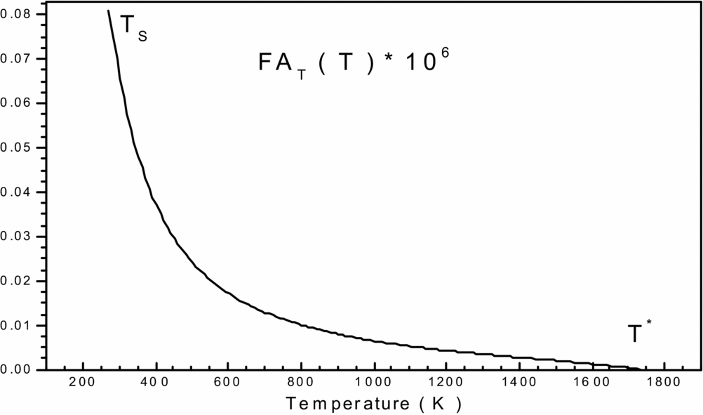
Figure 1. Variation of function FAT(T, ρ) in the interval [TS, T*] versus T 0.
The expressions of the partial derivative in the second member of Equation (27) can be calculated for the Berthelot equation. Then, the Equation (27) becomes for the Berthelot equation by:
 $$\begin{equation}
{c_p}(T,\rho ) = {c_{{P_{PG}}}}\left[ {1 + \left( {\frac{{{\gamma _{PG}} - 1}}{{{\gamma _{PG}}}}} \right)\left\{ \begin{array}{l} {\left( {\frac{\theta }{T}} \right)^2}\frac{Z}{{{{\left( {1 - Z} \right)}^2}}} \\
+\frac{{2a\rho }}{{R{T^2}}}\left[ {1 + \frac{{\left( {\frac{{2 - b\rho }}{{1 - b\rho }} + \frac{{a\rho }}{{2R{T^2}}}} \right)}}{{\frac{1}{{{{\left( {1 - b\rho } \right)}^2}}} - \frac{{2a\rho }}{{R{T^2}}}}}} \right] \end{array} \right\}} \right]
\end{equation}$$
$$\begin{equation}
{c_p}(T,\rho ) = {c_{{P_{PG}}}}\left[ {1 + \left( {\frac{{{\gamma _{PG}} - 1}}{{{\gamma _{PG}}}}} \right)\left\{ \begin{array}{l} {\left( {\frac{\theta }{T}} \right)^2}\frac{Z}{{{{\left( {1 - Z} \right)}^2}}} \\
+\frac{{2a\rho }}{{R{T^2}}}\left[ {1 + \frac{{\left( {\frac{{2 - b\rho }}{{1 - b\rho }} + \frac{{a\rho }}{{2R{T^2}}}} \right)}}{{\frac{1}{{{{\left( {1 - b\rho } \right)}^2}}} - \frac{{2a\rho }}{{R{T^2}}}}}} \right] \end{array} \right\}} \right]
\end{equation}$$The ratio of specific heat γ follows directly, of course, from Equations (28) and (26):
 $$\begin{equation}
\gamma (T,\rho ) = \left[ {\frac{{{c_p}(T,\rho )}}{{{c_v}(T,\rho )}}} \right]
\end{equation}$$
$$\begin{equation}
\gamma (T,\rho ) = \left[ {\frac{{{c_p}(T,\rho )}}{{{c_v}(T,\rho )}}} \right]
\end{equation}$$2.3 Critical cross-section area ratio
The equation of mass conservation is(Reference Rhyming3):
 $$\begin{equation}
\rho VA = cte
\end{equation}$$
$$\begin{equation}
\rho VA = cte
\end{equation}$$The differential of Equation (30) gives(Reference Fletcher12):
 $$\begin{equation}
\frac{{d\rho }}{\rho } + \frac{{dV}}{V} + \frac{{dA}}{A} = 0\,\, {\rm{and}}
\end{equation}$$
$$\begin{equation}
\frac{{d\rho }}{\rho } + \frac{{dV}}{V} + \frac{{dA}}{A} = 0\,\, {\rm{and}}
\end{equation}$$ $$\begin{equation}
\frac{{dA}}{A} = - \left( {\frac{{d\rho }}{\rho } + \frac{{dV}}{V}} \right)
\end{equation}$$
$$\begin{equation}
\frac{{dA}}{A} = - \left( {\frac{{d\rho }}{\rho } + \frac{{dV}}{V}} \right)
\end{equation}$$According to Equation (6), we can write:
 $$\begin{equation}
VdV = - C_S^2\frac{{d\rho }}{\rho }
\end{equation}$$
$$\begin{equation}
VdV = - C_S^2\frac{{d\rho }}{\rho }
\end{equation}$$Dividing Equation (33) by V 2, we have:
 $$\begin{equation}
\frac{{VdV}}{{{V^2}}} = - \frac{{C_S^2}}{{{V^2}}}\frac{{d\rho }}{\rho } \Rightarrow \frac{{dV}}{V} = - \frac{1}{{{M^2}}}\frac{{d\rho }}{\rho }
\end{equation}$$
$$\begin{equation}
\frac{{VdV}}{{{V^2}}} = - \frac{{C_S^2}}{{{V^2}}}\frac{{d\rho }}{\rho } \Rightarrow \frac{{dV}}{V} = - \frac{1}{{{M^2}}}\frac{{d\rho }}{\rho }
\end{equation}$$Replacing Equation (34) into Equation (32) we obtain:
 $$\begin{equation}
\frac{{dA}}{A} = \left( {\frac{{1 - {M^2}}}{{{M^2}}}} \right)\frac{{d\rho }}{\rho }
\end{equation}$$
$$\begin{equation}
\frac{{dA}}{A} = \left( {\frac{{1 - {M^2}}}{{{M^2}}}} \right)\frac{{d\rho }}{\rho }
\end{equation}$$Replacing Equation (7) into Equation (35) we obtain:
 $$\begin{equation}
\frac{{dA}}{A} = \left( {\frac{{1 - {M^2}}}{{{M^2}}}} \right)\,\left[ {\frac{{{C_P}(T,\rho )}}{{C_S^2}}dT + \frac{{{C_T}(T,\rho )}}{{C_S^2}}d\rho } \right]
\end{equation}$$
$$\begin{equation}
\frac{{dA}}{A} = \left( {\frac{{1 - {M^2}}}{{{M^2}}}} \right)\,\left[ {\frac{{{C_P}(T,\rho )}}{{C_S^2}}dT + \frac{{{C_T}(T,\rho )}}{{C_S^2}}d\rho } \right]
\end{equation}$$Finally,:
 $$\begin{equation}
\frac{{dA}}{A} = \left[ {\left( {\frac{{1 - {M^2}(T,\rho )}}{{{V^2}(T,\rho )}}.{C_P}(T,\rho )} \right)dT + \left( {\frac{{1 - {M^2}(T,\rho )}}{{{V^2}(T,\rho )}}.{C_T}(T,\rho )} \right)d\rho } \right]
\end{equation}$$
$$\begin{equation}
\frac{{dA}}{A} = \left[ {\left( {\frac{{1 - {M^2}(T,\rho )}}{{{V^2}(T,\rho )}}.{C_P}(T,\rho )} \right)dT + \left( {\frac{{1 - {M^2}(T,\rho )}}{{{V^2}(T,\rho )}}.{C_T}(T,\rho )} \right)d\rho } \right]
\end{equation}$$Substituting Equation (37) between the critical condition given by (T *, P *, ρ *, M* = 1 and A *), and supersonic status given by (T, P, ρ, M, A), we have:
 $$\begin{equation}
\int\limits_{{A^ * }}^A {\frac{{dA}}{A}} = \int\limits_{{T^ * }}^T {\left( {\frac{{1 - {M^2}(T,\rho )}}{{{V^2}(T,\rho )}}.{C_P}(T,\rho )} \right)dT} + \int\limits_{{\rho ^ * }}^\rho {\left( {\frac{{1 - {M^2}(T,\rho )}}{{{V^2}(T,\rho )}}.{C_T}(T,\rho )} \right)d\rho }
\end{equation}$$
$$\begin{equation}
\int\limits_{{A^ * }}^A {\frac{{dA}}{A}} = \int\limits_{{T^ * }}^T {\left( {\frac{{1 - {M^2}(T,\rho )}}{{{V^2}(T,\rho )}}.{C_P}(T,\rho )} \right)dT} + \int\limits_{{\rho ^ * }}^\rho {\left( {\frac{{1 - {M^2}(T,\rho )}}{{{V^2}(T,\rho )}}.{C_T}(T,\rho )} \right)d\rho }
\end{equation}$$Then:
 $$\begin{equation}
\frac{A}{{{A^ * }}} = Exp\left( {\int\limits_T^{{T^*}} {F{A_T}\left( {T,\rho } \right)dT} + \int\limits_\rho ^{{\rho ^*}} {F{A_\rho }\left( {T,\rho } \right)d\rho } } \right),
\end{equation}$$
$$\begin{equation}
\frac{A}{{{A^ * }}} = Exp\left( {\int\limits_T^{{T^*}} {F{A_T}\left( {T,\rho } \right)dT} + \int\limits_\rho ^{{\rho ^*}} {F{A_\rho }\left( {T,\rho } \right)d\rho } } \right),
\end{equation}$$with:
 $$\begin{equation}
F{A_T}(T,\rho ) = \frac{{{M^2}(T,\rho ) - 1}}{{{V^2}(T,\rho )}}.{C_P}(T,\rho )\,\,{\rm and}
\end{equation}$$
$$\begin{equation}
F{A_T}(T,\rho ) = \frac{{{M^2}(T,\rho ) - 1}}{{{V^2}(T,\rho )}}.{C_P}(T,\rho )\,\,{\rm and}
\end{equation}$$ $$\begin{equation}
F{A_\rho }(T,\rho ) = \frac{{{M^2}(T,\rho ) - 1}}{{{V^2}(T,\rho )}}.{C_T}(T,\rho )
\end{equation}$$
$$\begin{equation}
F{A_\rho }(T,\rho ) = \frac{{{M^2}(T,\rho ) - 1}}{{{V^2}(T,\rho )}}.{C_T}(T,\rho )
\end{equation}$$We note that in calculating the critical cross-sectional area ratio, we need to calculate the integral of certain functions where the analytical procedure is impossible, given the complexity of the functions to be integrated. So our interest is directed towards the numerical calculation. All our thermodynamic and geometric parameters, like M, V, A and CP, are functions according to both the temperature and density.
2.4 Expression of critical mass flow rate
The mass flow passing through a section is given by(Reference Rhyming3,Reference Comolet14) :
 $$\begin{equation}
\dot m = \int\limits_A {\rho {\rm{ }}V{\rm{cos}}\theta {\rm{ }}dA}
\end{equation}$$
$$\begin{equation}
\dot m = \int\limits_A {\rho {\rm{ }}V{\rm{cos}}\theta {\rm{ }}dA}
\end{equation}$$θ is the angle between the velocity vector with the normal to section A. If we divide Equation (42) by the quantityA *ρ0C 0S, to make the non-dimensional calculation, we have(Reference Zebbiche and Youbi6):
 $$\begin{equation}
\frac{{\dot m}}{{{A_*}{\rho _0}C_S^0}} = \int\limits_A {\frac{\rho }{{{\rho _0}}}{\rm{ }}\frac{{{C_s}}}{{C_S^0}}M{\rm{cos}}\theta \frac{{{\rm{ }}dA}}{{{A_*}}}}
\end{equation}$$
$$\begin{equation}
\frac{{\dot m}}{{{A_*}{\rho _0}C_S^0}} = \int\limits_A {\frac{\rho }{{{\rho _0}}}{\rm{ }}\frac{{{C_s}}}{{C_S^0}}M{\rm{cos}}\theta \frac{{{\rm{ }}dA}}{{{A_*}}}}
\end{equation}$$Given that the critical mass flow rate is constant, we can calculate at the throat of the nozzle. In this section, we have ρ = ρ*, A = A*, CS = C*S, M = 1 and θ = 0 degrees (horizontal flow). So, our relationship is the reduced equation:
 $$\begin{equation}
\frac{{\dot m}}{{{A_*}{\rho _0}C_S^0}} = \left( {\frac{{{\rho _*}}}{{{\rho _0}}}} \right)\left( {\frac{{C_S^*}}{{C_S^0}}} \right)
\end{equation}$$
$$\begin{equation}
\frac{{\dot m}}{{{A_*}{\rho _0}C_S^0}} = \left( {\frac{{{\rho _*}}}{{{\rho _0}}}} \right)\left( {\frac{{C_S^*}}{{C_S^0}}} \right)
\end{equation}$$Finally,
 $$\begin{equation}
\frac{{\dot m}}{{{A_*}{\rho _0}C_S^0}} = \left( {\frac{{\frac{{R{T_*}{\rho _*}}}{{{{\left( {1 - b{\rho _*}} \right)}^2}}} - \frac{{2a{\rho _*}^2}}{{{T_*}}} + \frac{{{\rho _*}^3{T_*}{{\left( {\frac{a}{{{T_*}^2}} + \frac{R}{{\left( {1 - b{\rho _*}} \right)}}} \right)}^2}}}{{{c_{{v_{gp}}}}\left\{ {1 + ({\gamma _{gp}} - 1){{\left( {\frac{\theta }{{{T_*}}}} \right)}^2}\frac{{{e^{\frac{\theta }{{{T_*}}}}}}}{{{{\left( {1 - {e^{\frac{\theta }{{{T_*}}}}}} \right)}^2}}} + \frac{{2a{\rho _*}}}{{R{T_*}^2}}} \right\}}}}}{{\frac{{R{T_0}{\rho _0}}}{{{{\left( {1 - b{\rho _0}} \right)}^2}}} - \frac{{2a{\rho _0}^2}}{{{T_0}}} + \frac{{{\rho _0}^3{T_0}{{\left( {\frac{a}{{{T_0}^2}} + \frac{R}{{\left( {1 - b{\rho _0}} \right)}}} \right)}^2}}}{{{c_{{v_{gp}}}}\left\{ {1 + ({\gamma _{gp}} - 1){{\left( {\frac{\theta }{{{T_0}}}} \right)}^2}\frac{{{e^{\frac{\theta }{{{T_0}}}}}}}{{{{\left( {1 - {e^{\frac{\theta }{{{T_0}}}}}} \right)}^2}}} + \frac{{2a{\rho _0}}}{{R{T_0}^2}}} \right\}}}}}} \right)
\end{equation}$$
$$\begin{equation}
\frac{{\dot m}}{{{A_*}{\rho _0}C_S^0}} = \left( {\frac{{\frac{{R{T_*}{\rho _*}}}{{{{\left( {1 - b{\rho _*}} \right)}^2}}} - \frac{{2a{\rho _*}^2}}{{{T_*}}} + \frac{{{\rho _*}^3{T_*}{{\left( {\frac{a}{{{T_*}^2}} + \frac{R}{{\left( {1 - b{\rho _*}} \right)}}} \right)}^2}}}{{{c_{{v_{gp}}}}\left\{ {1 + ({\gamma _{gp}} - 1){{\left( {\frac{\theta }{{{T_*}}}} \right)}^2}\frac{{{e^{\frac{\theta }{{{T_*}}}}}}}{{{{\left( {1 - {e^{\frac{\theta }{{{T_*}}}}}} \right)}^2}}} + \frac{{2a{\rho _*}}}{{R{T_*}^2}}} \right\}}}}}{{\frac{{R{T_0}{\rho _0}}}{{{{\left( {1 - b{\rho _0}} \right)}^2}}} - \frac{{2a{\rho _0}^2}}{{{T_0}}} + \frac{{{\rho _0}^3{T_0}{{\left( {\frac{a}{{{T_0}^2}} + \frac{R}{{\left( {1 - b{\rho _0}} \right)}}} \right)}^2}}}{{{c_{{v_{gp}}}}\left\{ {1 + ({\gamma _{gp}} - 1){{\left( {\frac{\theta }{{{T_0}}}} \right)}^2}\frac{{{e^{\frac{\theta }{{{T_0}}}}}}}{{{{\left( {1 - {e^{\frac{\theta }{{{T_0}}}}}} \right)}^2}}} + \frac{{2a{\rho _0}}}{{R{T_0}^2}}} \right\}}}}}} \right)
\end{equation}$$3.0 CALCULATION PROCEDURE
3.1 Stagnation mass density
After setting the values of the stagnation pressure and temperature, we need to calculate the stagnation mass density ρ0. The latter was calculated numerically from Berthelot's equation by the dichotomy method(Reference Demidovitch and Maron15). We can easily choose an interval [ρ1, ρ2] containing the density ρ0 and must satisfy F(ρ1)*F(ρ2) ⩽ 0. We can take ρ1 = 0 and ρ2 = ρ1 + step. Once this interval is determined, we can calculate ρ0 with a precision ε and a very small step. The value of ρ0 that is obtained depends on the precision ε and the step. The number of iterations (K), corresponding to the (ε) precision necessary to determine the stagnation mass density (ρ0) is given by(Reference Zebbiche and Youbi6):
 $$\begin{equation}
K = \frac{1}{{0.6931}}Log\left( {\frac{{Pas}}{\varepsilon }} \right) + 1
\end{equation}$$
$$\begin{equation}
K = \frac{1}{{0.6931}}Log\left( {\frac{{Pas}}{\varepsilon }} \right) + 1
\end{equation}$$If ε = 10−16, and the step = 10−4, the number of iterations (K) cannot exceed 41 iterations.
3.2 Determining the thermodynamic ratios:
Before determining the thermodynamic ratios, first numerically calculate the parameters of the static state. With a Mach number M-known, these static parameters can be found by solving a non-linear algebraic equation system formed by the Equations (1), (20) and (25). The calculation is done using Newton's algorithm(Reference Raltson and Rabinowitz16) with a numerical derivation of Equations (1), (20) and (25), first, with the temperature, and second, with the density. The calculation is started by putting the parameters of the static case of a perfect gas as an initial vector. For our algorithm, the derivation is done with a step equal to 10−4 and the calculation is made with a precision of ε = 10−8. The number of iterations cannot exceed 100K iterations.
Once these static parameters are determined using the calculation of thermodynamic ratios with a precision ε = 10−16, we divide the static parameters by our stagnation parameters to find the ratio of temperatures T/T 0, the pressure ratio P/P 0, the ratio of densities ρ/ρ 0, and the ratio of sound velocities CS/C 0S. This is done by replacing, in Equation (24), the parameters of the stagnation state T 0, P 0, ρ0 to find the stagnation speed of sound C 0S and all static parameters, such as T, P, ρ, to find the speed of sound.
3.3 Critical ratios
The stagnation state is given by the Mach number when equal to zero (M = 0). Then, the critical parameters which correspond to the temperature T 0 and the density ρ0 at the Mach number M = 1 (which is the case in the throat of the nozzle) can be determined. If we replace M = 1 in Equation (25), and solve the non-linear algebraic equation system formed by Equations (1), (20) and (25) by Newton's method(Reference Raltson and Rabinowitz16) putting the critical parameters Tc, Pc, ρc of the case of a perfect gas as an initial vector for starting the calculation, the derivation is made numerically for Equations (1), (20) and (25), first with the temperature, and second with the density, with a step equal to 10−4. The calculation is done with a precision ε = 10−8 and the number of iterations cannot exceed 100 iterations.
Once these critical parameters are determined, the calculation of thermodynamic ratios is made with a precision ε = 10−16. Divide these critical parameters by our stagnation parameters to find the critical temperature ratio, critical pressure ratio, the critical densities ratio, and the ratio of the speeds of sound. Then, replace the stagnation parameters T 0, P 0, ρ0 in Equation (24) to find the critical speed of the sound C*S. For the calculation of critical mass flow rate, we will do the same steps; we are replacing the stagnation parameters T 0, P 0, ρ0 and the critical parameters Tc, Pc, ρcdirectly into Equation (45).
3.4 Cross-sectional ratio
The determination of the cross-sectional areas given by the relationship in Equation (39) requires the numerical integration of functions FAT(T, ρ) in the interval [T, T*] and FAρ (T, ρ) in the interval [ρ, ρ*]. Note that the functions FAT (T, ρ) and FAρ(T, ρ) depend on the parameters T0 and ρ0.
To get an idea of the variation of each of the two previous functions, before making a decision on the choice of integration method, we carried and plotted the curves of variations. They are illustrated by Figs 1 and 2, respectively. We can conclude that the integration with constant step (pas) demand a very high discretization to have good precision for very fast variation to left ends of each interval (T = TS) and (ρ = ρs). For a good presentation to these ends, the tracing of these functions is chosen for the temperature T 0 = 2000K and MS = 6.00 (extreme supersonic). We note that the function FAT(T, ρ) has a very high derivative in the vicinity of the temperature TS. The condensation of nodes is then necessary to be adjacent to the temperature TS for this function. However, for the second function FAρ(T, ρ), we note that it decreases linearly when the density increases (see Fig. 2), which provides the mathematical integration method the ability to find the result of this integral.

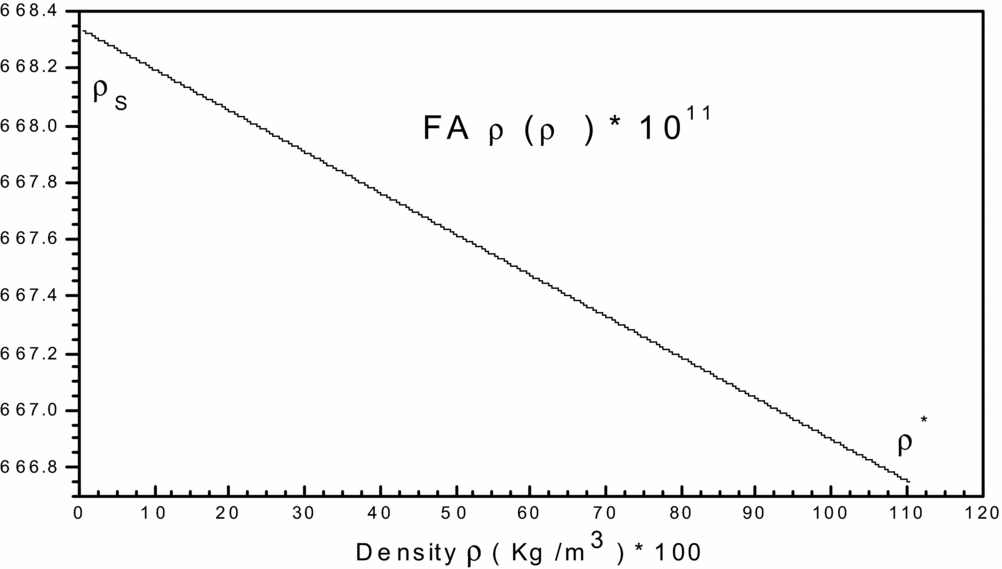
Figure 2. Variation of function FA ρ(T, ρ) in the interval [ρS, ρ*] versus T 0.
The purpose of this condensation is to calculate the value of the integral with a very high precision in a short time by minimizing the number of nodes of the integration method.
The integration method that was chosen is that of Simpson's method(Reference Zebbiche and Youbi5,Reference Demidovitch and Maron15) for the numerical calculation of integrals of functions FAT(T, ρ) and FAρ(T, ρ) in Equation (39). The condensation function is given by(Reference Zebbiche and Youbi6,Reference Raltson and Rabinowitz16) :
 $$\begin{equation}
{S_i} = {b_1}.{z_i} + \left( {1 - {b_1}} \right).\left[ {1 - \frac{{\tanh \left[ {{b_2}.\left( {1 - {z_i}} \right)} \right]}}{{\tanh \left( {{b_2}} \right)}}} \right],
\end{equation}$$
$$\begin{equation}
{S_i} = {b_1}.{z_i} + \left( {1 - {b_1}} \right).\left[ {1 - \frac{{\tanh \left[ {{b_2}.\left( {1 - {z_i}} \right)} \right]}}{{\tanh \left( {{b_2}} \right)}}} \right],
\end{equation}$$where:
 $$\begin{equation}
{z_i} = \frac{{i - 1}}{{N - 1}}1 \le i \le N
\end{equation}$$
$$\begin{equation}
{z_i} = \frac{{i - 1}}{{N - 1}}1 \le i \le N
\end{equation}$$After determining the condensation function, one can determine the temperature and density distribution by:
 $$\begin{equation}
{T_i} = {S_i}.\left( {{T_D} - {T_G}} \right) + {T_G}\quad {\rm{and}}
\end{equation}$$
$$\begin{equation}
{T_i} = {S_i}.\left( {{T_D} - {T_G}} \right) + {T_G}\quad {\rm{and}}
\end{equation}$$ $$\begin{equation}
{\rho _i} = {S_i}({\rho _D} - {\rho _G}) + {\rho _G}
\end{equation}$$
$$\begin{equation}
{\rho _i} = {S_i}({\rho _D} - {\rho _G}) + {\rho _G}
\end{equation}$$The temperature TD equals T* according to the function FAT(T, ρ), and TG equals TS. The density ρD equals ρ* for the function FAρ(T, ρ), and the density ρG equals ρS. If we take a value of b 1 close to zero (b 1 = 0.1) and b 2 = 2.0, we can condense the nodes to the left end of the interval TS. When we take values of b 1 close to 2 (e.g. b 1 = 1,9), the nodes may be condensed by the right end. For two subintervals the same lengths, we can take b 1 = 1.0.
Figure 3 shows the distribution of the nodes according to the choice of the value of b 1. Note that our interest is to condense the nodes to the left side (TS, ρS) with variation in functions FAT(T, ρ) and FAρ(T, ρ).
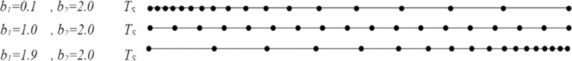
Figure 3. Representation of nodes condensation
3.5 Supersonic nozzle conception
For the supersonic nozzle application, it is necessary to determine the thrust coefficient CF. For the nozzle, given a uniform and parallel flow at the exit section, the thrust force and coefficient are(Reference Peterson and Hill17):
 $$\begin{equation}
F = \dot m{V_e} = \dot m{M_e}C_S^E,
\end{equation}$$
$$\begin{equation}
F = \dot m{V_e} = \dot m{M_e}C_S^E,
\end{equation}$$where:
 $$\begin{equation}
{C_f} = \frac{F}{{{P_0}{A_ * }}}
\end{equation}$$
$$\begin{equation}
{C_f} = \frac{F}{{{P_0}{A_ * }}}
\end{equation}$$At the throat, and from Equation (45):
 $$\begin{equation}
\frac{{\dot m}}{{{A_*}{\rho _0}C_S^0}} = \left( {\frac{{{\rho _*}}}{{{\rho _0}}}} \right)\left( {\frac{{C_S^*}}{{C_S^0}}} \right) \Rightarrow \dot m = {A_*}{\rho _0}C_S^0\left( {\frac{{{\rho _*}}}{{{\rho _0}}}} \right)\left( {\frac{{C_S^*}}{{C_S^0}}} \right)
\end{equation}$$
$$\begin{equation}
\frac{{\dot m}}{{{A_*}{\rho _0}C_S^0}} = \left( {\frac{{{\rho _*}}}{{{\rho _0}}}} \right)\left( {\frac{{C_S^*}}{{C_S^0}}} \right) \Rightarrow \dot m = {A_*}{\rho _0}C_S^0\left( {\frac{{{\rho _*}}}{{{\rho _0}}}} \right)\left( {\frac{{C_S^*}}{{C_S^0}}} \right)
\end{equation}$$Replacing Equation (53) into Equation (51), we obtain:
 $$\begin{equation}
F = \dot m{M_E}C_S^E = {A_*}{\rho _0}C_S^0\left( {\frac{{{\rho _*}}}{{{\rho _0}}}} \right)\left( {\frac{{C_S^*}}{{C_S^0}}} \right){M_E}C_S^E
\end{equation}$$
$$\begin{equation}
F = \dot m{M_E}C_S^E = {A_*}{\rho _0}C_S^0\left( {\frac{{{\rho _*}}}{{{\rho _0}}}} \right)\left( {\frac{{C_S^*}}{{C_S^0}}} \right){M_E}C_S^E
\end{equation}$$Replacing Equation (54) into Equation (52), we have:
 $$\begin{equation}
{C_f} = {M_E}(T,\rho ).\left( {\frac{{{\rho _*}}}{{{\rho _0}}}} \right).\frac{{{\rho _0}}}{{{P_0}}}C_S^*({T_ * },{\rho _ * }).C_S^E(T,\rho )
\end{equation}$$
$$\begin{equation}
{C_f} = {M_E}(T,\rho ).\left( {\frac{{{\rho _*}}}{{{\rho _0}}}} \right).\frac{{{\rho _0}}}{{{P_0}}}C_S^*({T_ * },{\rho _ * }).C_S^E(T,\rho )
\end{equation}$$3.6 Error of perfect gas model
The mathematically perfect gas model is developed on the basis of the specific heat CP and ratio γ as constants, which gives acceptable results for low temperature. According to this study, we can notice a difference of the given results between the perfect gas (PG) model and the model developed here (RG). The error given by the PG model compared to our RG model can be calculated for each parameter. Then, for each value (P 0, T 0, M), the ε error can be evaluated by the following relationship(Reference Zebbiche, Salhi and Boun-jad18):
 $$\begin{equation}
{\varepsilon _{Parameter}}(\% ){\rm{ }} = \left| {{\rm{ }}1 - \frac{{Paramete{r_{PG}}\left( {{P_0},{T_0},M} \right)}}{{Paramete{r_{RG}}\left( {{P_0},{T_0},M} \right)}}{\rm{ }}} \right| \times 100
\end{equation}$$
$$\begin{equation}
{\varepsilon _{Parameter}}(\% ){\rm{ }} = \left| {{\rm{ }}1 - \frac{{Paramete{r_{PG}}\left( {{P_0},{T_0},M} \right)}}{{Paramete{r_{RG}}\left( {{P_0},{T_0},M} \right)}}{\rm{ }}} \right| \times 100
\end{equation}$$As a rule for the aerodynamic application, the error should be lower than 5%.
4.0 RESULTS AND COMMENTS
4.1 Results for real gas characteristics
Figure 4 illustrates the variation of the stagnation mass density calculated numerically by the dichotomy method versus T 0 for a few values of the stagnation pressure, with a precision of ε = 10−16. We can notice a decrease in the density when T 0 increases. For low values of T 0, we note that the results obtained by the real gas model move away from those obtained by the perfect gas model and approach at big values of T 0. We also note that the increase of the stagnation pressure causes an increase in the mass density; in this case, for low values of the temperature, we find the results obtained by the real gas move away from those obtained by the perfect gas model and nearer to big values of the temperature T 0. Thus, this variation demonstrates the effects of molecular size and intermolecular force bound by Berthelot's equation. However, in short, we can say that both models take the same shape of decreasing. Otherwise, we have clearly seen that our model RG represents the closest model to the experimental data(Reference Haynes19,Reference Hilsenrath, Beckett, Benedict, Fano, Hoge, Masi, Nuttall, Touloukian and Woolley20) and gives more validity to the RG model.
Figure 4. Variation of density ρ0 versus T 0.
Figure 5 illustrates the variation of the relative error in percentage given by the mass density ρ 0, between the real gas and perfect gas models, versus the stagnation temperature for a few values of the stagnation pressure.
Figure 5. Variation of the relative error versus T 0. .
For instance, it is obvious that if one opts with an error of less than 5%, either the PG model can be used until P 0 is less than 4 bar for any value of the stagnation temperature, or until T 0 = 1000K for any value where P 0 does not exceed 200 bar. If an author accepts an error greater than 5%, we can use the PG model in the range of moderate P 0 and T 0.
We have clearly seen that the error hereby depends on the values of T 0 and P 0. The error increased when P 0 would increase; that demonstrates the effect of molecular size (a) and the intermolecular force (c) in Berthelot's equation. For instance, if T 0 = 250K, the use of the PG model will give us a relative error equal to ε = 12.298% for P 0 = 100 bar, which yields a difference of 16.20Kg/m3 between our two models (ε = 1.36% for P 0 = 10 bar and ε = 0.14% for P 0 = 1 bar).
We can also note that at high pressure and low temperature, the error ε is greater. This position is interpreted by the inability to use the PG model until T 0 = 1000K for aeronautical applications if we accept a relative error less than 5%. But if the temperature T 0 is higher, the error decreases progressively; in this case, we can use the model PG independently to P 0.
Figure 6 shows the variation of specific heat CP versus the stagnation temperature until T 0 = 3000K for some values of the pressure P 0 and for the HT, PG and RG models. The high temperature graph is presented using polynomial interpolation. At low temperatures, we observe that both HT and PG models take the exact same shape, except our model RG that varies depending on the pressure P 0. For example, when T 0 = 100K, we find CP = 1001.289J/Kg K for the PG model, CP = 1001.159J/Kg K for the HT model, and CP = 1001.536, 1003.602 and 1014.94 J/Kg k for the RG model corresponding to pressures P 0 = 1, 10 and 100 bar. In this case, we can say that both models PG and HT are considered calorically perfect. Otherwise, when the temperature T 0 increases, we see that both HT and RG models increase and take the same shape until 1300K. In this case, we can say that both HT and RG are calorically imperfect.
Figure 6. Variation of the specific heats CP(T, ρ) versus stagnation temperature T 0.
We also note that the CP remains constant for the RG model for any values of the pressure P 0, and always under the HT model. At T 0 equals 1300K, we can see the difference between HT and RG, which demonstrates the effects of molecular size, the intermolecular force and the constant θ of molecular vibrational energy. This variation will influence the thermodynamic parameters of the flow; in this case, we can say that our model is thermally and calorically imperfect. Therefore, the results presented by the PG model is given by Reference AndersonRefs 2, Reference Rhyming3 and Reference Shapiro9, and the results presented by the HT model is given by Reference Zebbiche and YoubiRefs 5 and Reference Zebbiche and Youbi6. Otherwise, we have clearly seen that our model RG is the model closest to the experimental data(Reference Hilsenrath, Beckett, Benedict, Fano, Hoge, Masi, Nuttall, Touloukian and Woolley20), which gives more validity to the RG model.
Figure 7 shows the variation of the specific heat ratio γ versus the stagnation temperature until 3000K for some values of the pressure P 0, and for the HT, PG and RG models. The high temperature model graph is presented using polynomial interpolation. At low temperatures, we observe that both HT and PG models take the same shape, except our model RG varies depending on pressure P 0. For example, when T 0 = 100K, we find γ = 1.402 for the PG model, γ = 1.40188 for the HT model, and γ = 1.40218, 1.40367 and 1.4092 for the RG model with corresponding pressures P 0 = 1, 10 and 100 bar. Otherwise, when the temperature T 0 increases, we see that both HT and RG models decrease and take the same shape until 1300K. However, if the temperature T 0 increases above 1300K, we can see the difference between HT and RG models, which demonstrates the effects of molecular size (a), the intermolecular force and the molecular vibrational energy constant θ. This variation will influence the thermodynamic parameters of the flow. Otherwise, the specific heat ratio γ of the RG model remains constant for any value of stagnation pressure P 0 and always upper and higher than the HT model. Otherwise, we have clearly seen that our model RG is the model nearest to the experimental data(Reference Hilsenrath, Beckett, Benedict, Fano, Hoge, Masi, Nuttall, Touloukian and Woolley20), which gives more validity to the RG model.
Figure 7. Variation of the specific heats ratio γ versus stagnation temperature.
Figure 8 represents the variation of the CT coefficient versus the stagnation temperature until 3000K, for some values of the pressure P 0. Consider an idea about the variation of this parameter. The CT coefficient increases linearly with temperature T 0, also increasing when the pressure P 0 increases. For instance, at T 0 = 1500K, we have CT = 462.23, 464.33, 473.74 and 485.64 (J/Kg K), respectively, for stagnation pressure equal to 1 bar, 10 bar, 50 bar and 100 bar. Finally, this figure proves that the CT coefficient depends on the stagnation temperature and pressure. Therefore, the CT coefficient binds to our RG model and equals zero for the PG and HT models.
Figure 8. Variation of CT coefficient versus stagnation temperature.
Figure 9 represents the variation of the sound velocity CS versus the stagnation temperature until 3000K for some values of the P 0, and for the HT, PG and RG models. We have clearly seen that the increasing of the temperature T 0 for all models causes an increase of the sound velocity CS. At low temperatures, we observe that both HT and PG models almost take the same shape, except our RG model, which depends on the pressure P 0, where, for example, it is especially important for P 0 = 100 bar. For instance, when T 0 = 700K, we find CS = 530.81ms−1 for the PG model, CS = 523.45ms−1 for the HT model, and CS = 524.12, 526.67 and 552.17ms−1 for the RG model with corresponding pressures P 0 = 1, 10and 100 bar. Otherwise, when temperature T 0 increases, we can see the difference between the three models PG, HT and RG. For example, when T 0 = 2000K, we find CS = 897.23ms−1 for the PG model, CS = 863.22ms−1 for model HT, and CS = 864.72, 866.19 and 880.93ms−1 for the RG model, respectively corresponding to the pressures P 0 = 1, 10 and 100 bar. This variation will influence the thermodynamic parameters of the flow, which shows the effect of molecular size (a), the intermolecular force (b), and the molecular vibrational energy constant (θ). However, in short, we can say the sound velocity of our RG model depends on the temperature T 0 and the pressure P 0.
Figure 9. Variation of the Sound Velocity CS versus the temperature.
4.2 Results for the supersonic parameters
Figure 10 shows the variation of the temperature ratio T/T 0 versus the Mach number for HT, PG and RG models, and for some values of the pressure P 0 correspondent to 1, 10 and 50 bar. We note that the increasing of the Mach number for different models leads to a decrease of the temperature ratio. We also see the variation of the stagnation temperature values for T 0 = 1000K, 2000K and 3000K, influencing the temperature ratios, which is not the case of the perfect gas model. For example, if M = 3.0 and T 0 = 2000K, T/T 0 = 0.35599 for the PG model, T/T 0 = 0.40569 for the model HT, and T/T 0 = 0.40467, 0.40479 and 0.40533 for the RG model, respectively corresponding to the pressures 1, 10 and 50 bar, with relative errors between the HT model and our model RG that are equal to ε = 0.25% for P 0 = 1 bar, ε = 0.22% for P 0 = 10 bar, and ε = 0.09% for P 0 = 50 bar. In our figure, the curve of the PG model indicates that the perfect gas is cooling the flow compared to the real thermodynamic behaviour of the gas. The numerical values presented are determined with better precision when ε = 10−16.
Figure 10. Variation of T/T 0 versus Mach number.
Figure 11 shows the variation of the mass density ratios ρ/ρ 0 versus the Mach number for the HT, PG and RG models, and for some values of the pressure P 0 = 1, 10 and 50 bar. We note that increasing the Mach number for different models causes a decrease of mass density ratios. We also see that the variation of the stagnation temperature values for T 0 = 1000K, 2000K and 3000K, influences these ratios, which is not the case for the perfect gas model. For example, if M = 2.5 and T 0 = 2000K, then ρ/ρ 0 = 0.1321 for the PG model, ρ/ρ 0 = 0.11149 for the HT model, and ρ/ρ 0 = 0.11188, 0.11212 and 0.11317 for the RG model, with respectively corresponding pressures 1, 10 and 50 bar, with relative errors between the HT model and our model RG equal to ε = 0.348% for P 0 = 1 bar, ε = 0.562% for P 0 = 10 bar, and ε = 1.485% for P 0 = 50 bar. The numerical values presented are determined with better precision when ε = 10−16.
Figure 11. Variation of ρ/ρ0 versus Mach number.
Figure 12 represents the variation of the pressure ratios P/P 0 versus the Mach number for the HT, PG and RG models, and for some values of the pressure P 0 equal to 1, 10 and 50 bar. We see the increase of the Mach number for different models causes a decrease of pressure ratios. We can also see the variation of the stagnation temperature values for T 0 = 1000K, 2000K and 3000K influences the pressure ratio, which is not the case for the perfect gas model. For example, if M = 2.0 and T 0 = 2000K, P/P 0 = 0.12775 for the PG model, P/P 0 = 0.12872 for the HT model, and P/P 0 = 0.12874, 0.12878 and 0.12897 for the RG model, respectively corresponding to the pressures 1 bar, 10 bar and 50 bar, with relative errors between the HT model and our model RG equal to ε = 0.015% for P 0 = 1 bar, ε = 0.047% for P 0 = 10 bar, and ε = 0.194% for P 0 = 50 bar. The numerical values presented are determined with better precision when ε = 10−16.
Figure 12. Variation of P/P 0 versus Mach number.
Figure 13 represents the variation of the sound velocity ratio CS/C 0S versus the Mach number for HT, PG and RG models, and for some values of the pressure P 0 equal to 1, 10 and 50 bar. We see that the increase of the Mach number for different models causes a decrease of the sound velocity ratios and the variation of the stagnation temperature. When T 0 = 1000K, 2000K and 3000K, we see influences on the sound velocity ratio, which is not the case for the perfect gas model. For instance, if M = 3.0 and T 0 = 3000K, then, CS/C 0S = 0.59666 for the PG model, CS/C 0S = 0.6594 for the HT model, and CS/C 0S = 0.65507, 0.65443, 0.6516 for the RG model, respectively corresponding to the pressures 1 bar, 10 bar and 50 bar, with relative errors between the HT model and our RG model at ε = 0.66% for P 0 = 1 bar, ε = 0.76% for P 0 = 10 bar, and ε = 1.20% for P 0 = 50 bar. Therefore, when the stagnation pressure increases, the sound velocity obtained by the RG model moves away from those obtained by the HT model, which is most remarkable for a higher stagnation pressure greater or equal to 50 bar. This shows the effect of the stagnation pressure on the thermodynamic parameters and the numeric values presented are determined with better precision when ε = 10−16.
Figure 13. Variation of the sound velocity ratio CS/C 0S versus Mach number.
4.3 Results for the critical parameters
Figure 14 shows the variation of critical temperature ratios T */T 0 versus the stagnation temperature T 0, for the HT, PG and RG models, and for some values of the pressure P 0 equal to 1, 10 and 50 bar. We note that the increase of the stagnation temperature for different models leads to an increase of critical temperature ratios T */T 0. This sort of increase becomes significant when the value of T 0 is high, which is not the case for the perfect gas model. We can also see that critical temperature ratios T */T 0 obtained by our RG model are always lower than those obtained by the HT model, which gives our model more cooling than the model HT, and the increasing of P 0 leads to a decrease of critical temperature ratios T */T 0. Otherwise, since the stagnation temperature T 0 is greater than 2000K, the three curves of our RG model are approaching and moving away when the temperature T 0 decreases This remoteness becomes significant when the stagnation temperature is lower than 1000K, and is most noteworthy for a stagnation pressure greater or equal to 50 bar, which shows the effect of P 0 on critical flow parameters., The numerical values presented are determined with a better precision of ε = 10−16.
Figure 14. Variation of T*/T 0 versus T 0.
Figure 15 shows the variation of critical mass density ρ */ρ 0 versus the stagnation temperature for the HT, PG and RG models, and for some values of the pressure P 0 equal to 1, 10 and 50 bar. We note that the increase of the stagnation temperature for different models leads to a decrease of critical mass density ρ */ρ 0. This sort of decrease becomes considerable when the value of T 0 is less than 1400K, which is not the case for the perfect gas model. We can also see that the critical mass density ratios ρ */ρ 0 obtained by our model RG are always higher than those obtained by the HT model, and the increasing of the stagnation pressure P 0 leads to an increase of critical mass density ρ */ρ 0. Otherwise, since the stagnation temperature is greater than 2000K, the three curves of our RG model are approaching and moving away when the stagnation temperature decreases. This remoteness becomes significant when the T 0 is lower than 1000K, and most noteworthy for a stagnation pressure greater or equal to 50 bar, which shows the effect of the stagnation pressure P 0 on critical flow parameters. The numerical values presented are determined with a better precision of ε = 10−16.
Figure 15. Variation of ρ*/ρ0 versus T 0.
Figure 16 shows the variation of the critical pressure ratios P */P 0 versus T 0, for the HT, PG and RG models, and for some values of the pressure P 0 equal to 1, 10 and 50 bar. We note that the increase of T 0 for different models leads to an increase of the critical pressure ratios P */P 0. This sort of increase becomes significant when the value of T 0 is high, which is not the case for the perfect gas model. We can also see that the critical pressure ratio obtained by our RG model is always lower than those obtained by the HT model, and when the P 0 increases, the critical pressure ratios P */P 0 decrease, and that is mathematically true. Otherwise, since T 0 is greater than 2000K, the three curves of our RG model are approaching and moving away when T 0 decreases. This remoteness becomes significant when the T 0 is lower than 1000K, and most noteworthy for a stagnation pressure greater or equal to 50 bar, which shows the effect of the stagnation pressure P 0 on critical flow parameters. Numerical values presented are determined with a better precision of ε = 10−16.
Figure 16. Variation of P*/P 0 versus T 0.
Figure 17 shows the variation of the critical sound velocity ratios C*S/CS 0 versus T 0, for the HT, PG and RG models, and for some values of the pressure P 0 equal to 1, 10 and 50 bar. We note that the increase of the stagnation temperature T 0 for different models leads to an increase of critical sound velocity ratios C*S/CS 0. This sort of increase becomes significant when the value of T 0 is high, which is not the case for the perfect gas model. We can also remark that the critical sound velocity ratios C*S/CS 0 obtained by our model RG are always lower than those obtained by the HT model, and when the stagnation pressure increases, the critical sound velocity ratios C*S/CS 0 decrease. Otherwise, since the stagnation temperature T 0 is greater than 2000K, the three curves of our RG model are approaching and moving away when the temperature T 0 decreases. This remoteness becomes significant when T 0 is lower than 1000K, and most noteworthy for a stagnation pressure greater or equal to 50 bar, which shows the effect of the stagnation pressure P 0 on critical flow parameters. Numerical values presented are determined with a better precision of ε = 10−16.
Figure 17. Variation of C*S/CS 0 versus T 0.
4.4 Results for the supersonic nozzle application
Figure 18 shows the variation of the thrust coefficient CF versus the exit Mach number for the HT, PG and RG models, and for some values of the pressure P 0 equal to 1, 10 and 50 bar. We note that the increasing of the Mach number for different models leads to an increase of thrust coefficients and the variation of the stagnation temperature (e.g. for T 0 = 1000K, 2000K and 3000K, there are influences on the CF). Therefore, the CF coefficient increases when T 0 increases, which is not the case for the perfect gas model. Otherwise, if the exit Mach number is less than MS = 2.0, we note that the three models, PG, HT and RG are confounded and moving away when MS increases. For instance, if Ms = 5.0 and T 0 = 3000K, CF = 1.65234 for the PG model, CF = 1.73381 for the HT model, and CF = 1.73114, 1.73094 and 1.73004 for the RG model, respectively corresponding to the pressures 1 bar, 10 bar and 50 bar, with relative errors between the HT model and our model RG equal to ε = 0.15% for P 0 = 1 bar, ε = 0.165% for P 0 = 10 bar, and ε = 1.22% for P 0 = 50 bar. Therefore, when the stagnation pressure increases, the thrust coefficient CF obtained by the RG model moves away from those obtained by the HT model. This is most remarkable for a stagnation pressure greater or equal to 50 bar, which shows the effect of the stagnation pressure on the thermodynamic parameters. The numeric values presented are determined with a better precision of ε = 10−16.
Figure 18. Variation of CF versus exit Mach number.
Figure 19 shows the variation of the critical cross-section area ratio A/A * versus the Mach number for HT, PG and RG models, and for some values of the pressure P 0 equal to 1, 10 and 50 bar. We note that the increasing of the Mach number for different models leads to an increase in the critical cross-section area ratio A/A *. We can also see the variation of the stagnation temperature values for T 0 = 1000K, 2000K and 3000K, influences the critical cross-section area ratio A/A *; the latter increases when T 0 increases, which is not the case for the perfect gas model. Otherwise, if the Mach number is lower than approximately M = 2.0, the three models PG, HT and RG are confounded and move away when the Mach number increases. For example, if M = 5.0 and T 0 = 3000K, then A/A * = 24.74917 for the PG model, A/A * = 40.38428 for the HT model, and A/A * = 39.87358, 39.82898 and 39.63156 for the RG model, respectively corresponding to the pressures 1, 10 and 50 bar, with relative errors between the HT model and our model RG equal to ε = 1.28% for P 0 = 1 bar, ε = 1.40% for P 0 = 10 bar, and ε = 1.90% for P 0 = 50 bar. Therefore, when P 0 increases, the critical cross-section area ratio A/A * obtained by the RG model moves away from those obtained by the HT model. This is most noteworthy for a stagnation pressure greater or equal to 50 bar, which shows the effect of P 0. The numeric values presented are determined with a better precision of ε = 10−16.
Figure 19. Variation of critical cross-section area ratio A/A * versus Mach number.
Figure 20 shows the variation of the non-dimensional critical mass flow rate through the critical cross-section versus the stagnation temperature T 0 for the HT, PG and RG models, and for some values of the pressure P 0 equal to 1, 10 and 50 bar. We note that the increase of T 0 for different models leads to an increase of the critical mass flow rate. This sort of increase becomes significant when T 0 is high, which is not the case for the perfect gas model. We can also remark that the critical mass flow rates obtained by our RG model are always lower than those obtained by the HT model; in addition, when the stagnation pressure P 0 increases, the critical mass flow decreases. Otherwise, since the stagnation temperature is greater than 2000K, the three curves of our RG model are approaching and moving away when T 0 decreases. This remoteness becomes significant when T 0 is lower than 1000K and noteworthy for a stagnation pressure greater or equal to 50 bar, which shows the effect of the stagnation pressure P 0 on critical flow parameters. With this variation between the three PG models, HT and RG will influence the value of the thrust force, especially if P 0 is great. This lack will influence the information given on the fuel lifetime, which will be less than the fuel lifetime given by the PG model and greater than the HT model. The numerical values presented are determined with a better precision of ε = 10−16.
Figure 20. Variation of the critical mass flow rate versus T 0.
Figure 21 shows the correction of the Mach number of the nozzle, given the exit Mach number Ms dimensioned on the basis of the PG model, corresponding respectively to T 0 = 1000K, 2000K and 3000K, and for P 0 = 1, 10 and 50 bar, versus the Mach number, between the RG and PG models.
Figure 21. Correction of the Mach number for RG model of a nozzle dimensioned on the PG model.
We have clearly seen that the variation of the Mach number depends on P 0 and T 0. If T 0 and P 0 increase, the Mach number of the real gas model decreases. For instance, if T 0 = 2000K at P 0 = 1 bar, when the Mach number delivered by the PG model MPG = 6.00, the Mach number delivered by the real gas model is MRG = 5.623. Now, if we have P 0 = 1 bar and T 0 = 1000K, and the Mach number delivered by the perfect gas model is MPG = 6.00, the Mach number delivered by the real gas model is MRG = 5.856. For these same values of stagnation pressure and T 0 = 3000K, we have MPG = 6.00, and the Mach number delivered by the real gas model is MRG = 5.500.
From these results, we can determine that the Mach number for a real gas can never attain the Mach number of the perfect gas under any condition. The decrease of the Mach number by increasing the stagnation pressure and temperature is quite normal because this increase causes an increase in the speed of sound and the latter is inversely proportional to the Mach number.
4.5 Error given by the perfect gas model
Figure 22 represents the variation of the relative error in percentage, which is given by the temperature ratio T/T 0, corresponding respectively to T 0 = 1000K, 2000K and 3000K, and for P 0 = 1, 10 and 50 bar, versus the Mach number, between the RG and PG models.
Figure 22. Variation of the relative error given by T/T 0 versus the Mach number.
It is obvious that the error depends on the values of P 0, T 0 and M; it increases when T 0 and P 0 increase. For instance, if T 0 = 2000K and M = 3.00, the use of the PG model will give us a relative error equal to ε = 12.028% for P 0 = 1 bar, ε = 12.054% for P 0 = 10 bar, and ε = 12.17% for P 0 = 50 bar, which gives a difference of 97.36K, 97.6K and 98.68K between the temperature values of the two models.
It is clear that if we chose an error, for example, lower than 5%, the PG model may be used if T 0 is less than 1000K and P 0 is below 90 bars for any value of the Mach number. If an author accepts an error greater than 5%, the PG model may be used in a moderate interval of M, P 0 and T 0.
It may be noted that, at low values of M, T 0 and P 0, the error ε is small. In Fig. 22(a) the error is below 5%. This position is interpreted by the possibility of using the PG model until T 0 = 1000K for the aeronautical applications; however, the stagnation pressure is well-moderate and does not exceed 90 bar, since we accept an error less than 5%. Otherwise, if the temperature T 0 is higher, the error increases progressively. Therefore, in this case, we can use the model PG independently to the temperature T 0, when the Mach number does not exceed M = 2.00 with an error of about 12%.
Figure 23 represents the variation of the relative error in percentage between the RG and PG models, which is given by the mass density ratio ρ/ρ 0, with T 0 = 1000K, 2000K and 3000K respectively corresponding to P 0 = 1, 10 and 50 bar, versus the Mach number.
Figure 23. Variation of the relative error given by ρ/ρ0 versus the Mach number.
It is obvious that the error depends on the values of P 0, T 0 and M; it increases when T 0 and P 0 increase. For example, if T 0 = 2000K and M = 3.00, the use of the PG model will give us a relative error equal to ε = 26.86% for P 0 = 1 bar, ε = 26.55% for P 0 = 10 bar, and ε = 25.19% for P 0 = 50 bar, which gives a difference of 0.0029Kg/m3, 0.028Kg/m3 and 0.134Kg/m3 between the mass density values of the two models.
It is clear that if we chose an error, for example, lower than 5%, the PG model may be used if T 0 is less than 1000K and P 0 is the pressure below 60 bar for any value of the Mach number. If an author accepts an error greater than 5%, the PG model may be used in a moderate interval of M, P 0 and T 0.
It may be noted that at low values of M and T 0, the error ε is small. We found the error is below 5%. This position is interpreted by the possibility of using the PG model until T 0 = 1000K (see Fig. 23(a)) for the aeronautical applications; however, a stagnation pressure is well-moderate and does not exceed 60 bar, since we accept an error less than 5%. Otherwise, if the temperature T 0 is high, the error increases progressively. Therefore, in this case, the model PG can be used independently to the temperature T 0, when the Mach number does not exceed M = 2.00 with an error about 12%.
Figure 24 represents the variation of the relative error in percentage between the RG and PG models, which is given by the pressure ratio P/P 0, with T 0 = 1000K, 2000K and 3000K respectively corresponding to P 0 = 1, 10 and 50 bar, versus the Mach number.
Figure 24. Variation of the relative error given by P/P 0 versus the Mach number.
It obvious that the error depends on the values of P 0, T 0 and M; it increases when T 0 and P 0 increase. For example, if T 0 = 2000K and M = 4.00, the use of the PG model will give us a relative error equal to ε = 24.39% for P 0 = 1 bar, ε = 24.22% for P 0 = 10 bar, and ε = 23.44% for P 0 = 50 bar, giving a difference of pressure values 0.0013 bar, 0013 bar and 0065 bar between the two models. However, the error is ε = 0.001% if the Mach number M = 1.8, T 0 = 1000K and P 0 = 1 bar; ε = 0.1% at M = 2.1, T 0 = 2000K and P 0 = 1 bar; ε = 0.3% at M = 2.2, T 0 = 3000K and P 0 = 1 bar; ε = 0.005% at M = 1.8, T 0 = 1000K and P 0 = 10 bar; ε = 0.05% at M = 2.1, T 0 = 2000K and P 0 = 10 bar; ε = 0.27% at M = 2.2, T 0 = 3000K and P 0 = 10 bar; ε = 0.08% at M = 1.8, T 0 = 1000K and P 0 = 50 bar; ε = 0.13% at M = 2.1, T 0 = 2000K and P 0 = 50 bar; and, ε = 0.11% at M = 2.2, T 0 = 3000K and P 0 = 50 bar. We conclude that we can reduce the error of the pressure ε < 1.0%, if we take an interval of the Mach number between M = 1.8 and M = 2.2. Therefore, in this interval we can say that our errors are instantaneously independent of P 0 and T 0.
It is clear that if we choose an error, for example, lower than 5%, the PG model may be used, if T 0 is less than 1000K and the pressure P 0 is greater than 1 bar for any value of the Mach number. If an author accepts an error greater than 5%, the PG model may be used with a moderate interval of M, P 0 and T 0.
It may be noted that, at values of M less than 2.6, the error ε is small. In those figures we find the error is below 5%. This position is interpreted by the possibility of using the PG model until T 0 = 3000K for the aeronautical applications, if we accept an error less than 5%. Otherwise, if the temperature T 0 is high, the error increases progressively. Therefore, the model PG may be used independently to the temperature T 0, when the Mach number does not exceed M = 3.00 with an error about 12%.
Figure 25 represents the variation of the relative error in percentage, which is given by the sound velocity ratio CS/C 0S, respectively corresponding to T 0 = 1000K, 2000K, and 3000K, and for P 0 = 1, 10, and 50 bar, versus the Mach number, between the RG and PG models.
Figure 25. Variation of the relative error given by CS/C 0S versus the Mach number.
We have clearly seen that the error depends on the values of P 0, T 0 and M; it increases when T 0 increases and decreases when P 0 increases. For example, if T 0 = 2000K and M = 3.00, the use of the PG model will give us a relative error equal to ε = 8.00% for P 0 = 1 bar, ε = 7.86% for P 0 = 10 bar, and ε = 7.26% for P 0 = 50 bar.
It is clear that if we chose an error, for example, lower than 5%, the PG model may be used, if T 0 is less than 1000K and the pressure P 0 is greater than 1 bar for any value of the Mach number. If an author accepts an error greater than 5%, the PG model may be used in a moderate interval of M, P 0 and T 0.
It may be noted that, at low values of M and T 0, the error ε is small. In those figures we find the error is below 5%. This position is interpreted by the possibility of using the PG model until T 0 = 1000K for the aeronautical applications. The stagnation pressure is well-moderate, if we accept an error less than 5%. Otherwise, if the temperature T 0 is higher, the error increases progressively; in this case, the model PG may be used independently to the temperature T 0, when the Mach number does not exceed M = 2.50 with an error of about 12%.
Figure 26 represents the variation of the relative error in percentage between the RG and PG models, which is given by the critical cross-section area ratio A/A *, respectively corresponding to T 0 = 1000K, 2000K and 3000K, and for P 0 = 1, 10 and 50 bar, versus the Mach number.
Figure 26. Variation of the relative error given by A/A * versus the Mach number.
We have clearly seen that the error depends on the values of P 0, T 0 and M; it increases when T 0 increases and decreases when P 0 increases. For example, if T 0 = 2000K and M = 3.00, the use of the PG model will give us a relative error equal to ε = 15.33% for P 0 = 1 bar, ε = 15.21% for P 0 = 10 bar, and ε = 14.70% for P 0 = 50 bar.
It is clear that if we chose an error, for example, lower than 5%, the PG model may be used, if T 0 is less than 1000K and the pressure P 0 is greater than 1 bar for any value of the Mach number (see Fig. 26(a)). If an author accepts an error greater than 5%, it can use the PG model in a moderate interval of M, P 0 and T 0.
It may be noted that, at low values of M and T 0, the error ε is small. In those figures we find the error is below 5%. This position is interpreted by the possibility of using the PG model until T 0 = 1000K for the aeronautical applications, with a well-moderate stagnation pressure, if we accept an error less than 5%. Otherwise, if the temperature T 0 is high, the error increases progressively; in this case, the model PG may be used independently to the temperature T 0, when the Mach number does not exceed M = 2.50 with an error of about 11%.
Figure 27 represents the variation of the relative error in percentage between the RG and PG models, which is given by the thrust coefficient CF, with T 0 = 1000K, 2000K and 3000K, respectively corresponding to P 0 = 1, 10 and 50 bar, versus the exit Mach number.
Figure 27. Variation of the relative error given by CF versus the exit Mach number.
We have clearly seen that the error depends on the values of P 0, T 0 and MS; it increases when T 0 and P 0 increase. For example, if T 0 = 2000K and M = 4.00, the use of the PG model will give us a relative error equal to ε = 2.95% for P 0 = 1 bar, ε = 2.94% for P 0 = 10 bar, and ε = 2.87% for P 0 = 50 bar, giving a difference of thrust coefficient values 0.0461, 0.0479 and 0.04428 between the two models. Otherwise, we note that the error ε = 0.024% if M = 2.0, T 0 = 1000K and P 0 = 1 bar; ε = 0.075% at M = 2.1, T 0 = 2000K, and P 0 = 1 bar; ε = 0.0142% at M = 2.1, T 0 = 3000K, and P 0 = 1 bar; ε = 0.0192% at M = 2.0, T 0 = 1000K, and P 0 = 10 bar; ε = 0.00732% at M = 2.1, T 0 = 2000K, and P 0 = 10 bar; ε = 0.0127% at M = 2.1, T 0 = 3000K, and P 0 = 10 bar; ε = 0.0042% at M = 2.0, T 0 = 1000K and P 0 = 50 bar; ε = 0.065% at M = 2.1, T 0 = 2000K, and P 0 = 50 bar; and, ε = 0.0062% at M = 2.1, T 0 = 3000K, and P 0 = 50 bar. We conclude that we can reduce the error ε < 1.0%, if we take an interval of Mach numbers between M = 2.0 and M = 2.1. Therefore, in this interval we can say that our errors are instantaneously independent of P 0 and T 0.
It is clear that if we choose an error, for example, lower than 5%, the PG model may be used, if T 0 is less than 3000K for any value of the pressure P 0 and the Mach number M (see Fig. 27). If an author accepts an error greater than 5%, the PG model may be used in a moderate interval of M, P 0 and T 0
CONCLUSION
From this study, we can quote the following points:
If we accept an error lower than 5%, which is generally the case for aerodynamic applications, we can study a supersonic flow using the relationships of a perfect gas, if T 0 is less than 1000K for any value of the Mach number, with a stagnation pressure well-defined and moderate, or when the Mach number is less than 2.00 for any value of T 0 up to approximately 3000K.
The PG model is represented by explicit and simple relations and does not require much time to make calculations. This is not the case for our RG model, where it is represented by solving a nonlinear algebraic equation. Solving a nonlinear algebraic equation system formed by three equations and derivation or integration of a complex analytical function, requires and takes more time for calculation, numerical programming, and data processing.
The main variables for our RG model are the temperature and the density- the temperature for the HT model and the Mach number for the PG model, because in our model RG, we have a nonlinear implicit equation relating T, ρ, and M.
We can choose another substance instead of air. Relations would remain valid except that it would be necessary to determine the constant of intermolecular force, molecular size, and the molecular vibrational energy constant Ө.
The cross-section area ratio presented by Equation (56) can be used as a source of comparison for the validation and verification of numerical results of the dimensions calculation of various supersonic nozzles. It provides a uniform and parallel flow at the exit section by the method of characteristics and the Prandtl Meyer function. Thermodynamic ratios can be used to determine the design parameters of the various shapes of nozzles under the basis of the RG model.
We can obtain the relations of a perfect gas model from our real gas model RG, by cancelling all constants of intermolecular force, molecular size, and the molecular vibrational energy constant Ө. In this case, the model PG becomes a particular case of our model RG.
We can also obtain the relations of a high temperature HT model from our model RG, by cancelling all constants of intermolecular force and molecular size. In this case, the model HT becomes a particular case of our model RG.
At low pressure, temperature and Mach number, the difference in results between the three models is small, which gives the opportunity to study the RG flow using the relations to PG. Contrariwise, when T 0 and P 0 increase, the PG theory starts giving results which move away progressively from the real cases where we need to use the RG model.
Our RG model is valid for any field or domain, especially at high pressure and low temperature field, or when the pressure is greater than 500 bar and for any value of the temperature. In these cases, there is a big difference in results between our RG model and the other HT and PG models (see Fig. 4), hence the necessity to use the RG model. However, our assumptions on the design of supersonic nozzles are based on pressure not to exceed 250 bar, because the increase in pressure influences the thickness of the nozzle, which influences the total mass of the nozzle. That is considered a major drawback for the design and for the fuel consumption.