1 Introduction
Filtration of a contaminant out of a fluid is vital for many industrial applications. Filtration technology is used in air conditioning and purifying systems, cars, vacuum cleaners, and the water treatment and food industries, to name a few. Filtration in these applications operates under the same principles (Neunzert & Prätzel-Wolters Reference Neunzert and Prätzel-Wolters2015). Contaminated fluid, such as air or water, is transported through a porous material, the filter medium. As contaminants pass through the filter medium, they come into contact with the surface of the porous medium and adhere, and, as a result, a cleaner fluid is produced. Filtration processes can be classified using four main characteristics: the transport mechanism, the operational set-up, the adsorption mechanisms and the filter-medium type.
1.1 Transport mechanisms and operational set-ups
The transport of contaminants though filter media can be driven by advection, diffusion and osmosis. In this work, we focus on the first two mechanisms. Depending on the transport mechanisms and the objectives of the filtration, the process can have different operational set-ups. A dead-end set-up, when the fluid flow is perpendicular to the filter medium, is used in advection-dominated filtration, while a cross-flow set-up, when the fluid flow is parallel to the filter medium, is commonly used for diffusion-dominated filtration. Moreover, when advection is present, the filtration can occur under a constant flow rate or a constant pressure drop. Some examples of applications that employ a constant flow rate are the air filters used in vacuum cleaners and air-conditioning systems (Fisk et al. Reference Fisk, Faulkner, Palonen and Seppanen2002). Filtration regimes in which a constant pressure drop is applied occur in the pharmaceutical and biotechnology industries – see, for example, Chen et al. (Reference Chen, Song, Qi, Li, Ghosh and Wan2015) and Goldrick et al. (Reference Goldrick, Joseph, Mollet, Turner, Gruber, Farid and Titchener-Hooker2017). One of the aims of this work is to discuss the mathematical modelling and to investigate numerically different transport mechanisms and set-ups.
1.2 Adsorption mechanisms
The adsorption mechanisms that usually act during the filtration process are diffusion, interception, impaction and gravitational settling. In addition, adsorption can be enhanced by, for example, electrostatic forces and chemical treatment of the filter medium. In this paper, we ignore the enhanced adsorption mechanisms and account for the standard mechanisms through a single so-called adsorption coefficient. For more discussions on the adhesive forces acting on the contaminant particles and their quantification, see, for example, Brown (Reference Brown1993) and Baron & Willeke (Reference Baron and Willeke2001).
1.3 Filter-medium types
Contaminant adsorption occurs at the pore level, or microscale, of the filter medium. Therefore, a natural question that arises is how the filtration performance is affected by the microstructure of the filter medium, that is, by the filter-medium type. The second aim of this paper is to investigate the influence of the microstructure on the filtration performance.
The effect of the filter-medium type has been investigated in different studies using a microscale approach with a fully resolved microstructure of filter media – see, for example, Fotovati, Tafreshi & Pourdeyhimi (Reference Fotovati, Tafreshi and Pourdeyhimi2010), Sambaer, Zatloukal & Kimmer (Reference Sambaer, Zatloukal and Kimmer2012), Becker et al. (Reference Becker, Wiegmann, Hahn and Lehmann2013), Robinson & Bruna (Reference Robinson and Bruna2015), Li, Shen & Li (Reference Li, Shen and Li2016) and Iliev et al. (Reference Iliev, Lakdawala, Nessler, Prill, Vutov, Yang and Yao2017) and references therein. Some of these studies track each particle individually using a Lagrangian approach, while others treat the contaminant as a continuum, which is possible if the particles are sufficiently small in comparison with the fibre size. Becker et al. (Reference Becker, Wiegmann, Hahn and Lehmann2013) evolve the microstructure as time progresses, while the other studies mentioned above consider only the initial filtration, namely before the adsorbed contaminants begin to influence the porous-medium microstructure. In general, the microscale approach provides detailed information about the filtration process, but it is computationally very expensive. Using this approach, we can only consider a small representative volume of the filter, and so this does not provide us with information about the behaviour of the entire filter medium. Even if we can resolve the whole thickness, due to the computational cost, only a very limited number of simulations can be performed, which makes the microscale approach unsuitable for comprehensive studies with different kinds of microstructures.
Filtration problems are also commonly modelled using a macroscale approach (Lakdawala Reference Lakdawala2010; Manikantan & Gunasekaran Reference Manikantan and Gunasekaran2013; Krupp et al. Reference Krupp, Please, Kumar and Griffiths2017). Here, the filter is modelled as a continuum and its characteristics are accounted for via empirical macroscopic parameters. Macroscale models are popular because one can relatively cheaply simulate the whole filtration process and various operational set-ups. Hence, unlike microscopic models, they are suitable for predictive studies. On the other hand, studying different types of filter media using this approach would require supplementing the simulations with experimental measurements, which are time-demanding and expensive to carry out. Hence, the macroscale approach is impractical for such a study.
A multiscale approach combines the advantages of both micro- and macroscale methods. Starting from a microscale model, the multiscale approach uses an upscaling method to derive a simple model at the macroscale that can be solved easily and used in predictive and comprehensive studies. But since the model is derived from a microscale model, its parameters bear a direct relation to the microscale features (Hornung Reference Hornung1996). For these reasons, multiscale models have become a popular tool in mathematical modeling – see, for example, Allaire et al. (Reference Allaire, Brizzi, Dufrêche, Mikelić and Piatnitski2014), Iliev, Lakdawala & Printsypar (Reference Iliev, Lakdawala and Printsypar2014), Ray, Elbinger & Knabner (Reference Ray, Elbinger and Knabner2015), Schmuck & Bazant (Reference Schmuck and Bazant2015) and Dalwadi, Bruna & Griffiths (Reference Dalwadi, Bruna and Griffiths2016).
Let us discuss three studies using the multiscale approach that are the most relevant to the work in this paper. Iliev et al. (Reference Iliev, Lakdawala and Printsypar2014) use a volume averaging approach, which yields the macroscopic equations via local averages in the form of volume integrals. The proposed model accounts for the microscale features of the filtration while modelling a whole filter element, that is, a casing for the filter medium with an inlet for the contaminated fluid and an outlet for the filtered fluid. However, the computational complexity of the resulting model is still quite challenging, requiring resolution of the filter-medium thickness at the microscale in addition to performing separate simulations for multiple locations in the filter medium. Thus, while this model is good to understand the effect of the microstructure on the filtration behaviour for a single set of parameters, performing studies for different types of microstructure using such a model is not practical.
The models by Ray et al. (Reference Ray, Elbinger and Knabner2015) and Dalwadi et al. (Reference Dalwadi, Bruna and Griffiths2016) employ the method of multiple scales, which assumes a separation of scales and averages the microscale variations. Both papers consider the flow and particle transport problems in an evolving porous medium, and Ray et al. (Reference Ray, Elbinger and Knabner2015) also accounts for a general interaction potential between fibres and particles (such as an electrostatic potential). Their multiscale models consist of a coupled system of equations for the flow and transport, with the effective parameters determined by solving the so-called cell problems in a microscopic unit cell. The model by Ray et al. (Reference Ray, Elbinger and Knabner2015) considers a more general microstructure using a level-set framework, but the drawback is that the microscopic and macroscopic problems are fully coupled, meaning that the cell problems have to be solved for each point in space and time. Under certain simplifications, namely no interaction potential and a quasi-periodic microstructure with unidirectional fibres that grow radially due to contaminant deposition, the model by Ray et al. (Reference Ray, Elbinger and Knabner2015) reduces to the one derived by Dalwadi et al. (Reference Dalwadi, Bruna and Griffiths2016). Under these assumptions, the cell problems depend only on the porosity and so the microscopic and macroscopic problems decouple, resulting in a more efficient simulation. On the other hand, the applicability of the model from Dalwadi et al. (Reference Dalwadi, Bruna and Griffiths2016) is limited due to its consideration only of microstructures of filter media with monodisperse fibres located on a regular lattice. Moreover, under their model assumptions, the simulation must be stopped when two fibres come in contact due to contaminant deposition.
1.4 Overview
In this paper, we use the method of multiple scales to study the effect of the filter microstructure in various filtration regimes. We are concerned with non-woven filter media, which is one of the most common filter-medium types (see Brown Reference Brown1993; Hutten Reference Hutten2015). The non-woven medium is a sheet made from directionally or randomly oriented fibres bonded together by chemical, mechanical, heat or solvent treatment. The contaminant transport is driven by diffusion and advection with the fluid and described using a continuum approach.
Our set-up is similar to the one in Dalwadi et al. (Reference Dalwadi, Bruna and Griffiths2016). In that paper the authors assumed that fibres are arranged in a simple quasi-periodic structure (a hexagonal lattice), and that all fibres have the same radius in a given unit cell. But real filter media have fibres with some diameter distribution, that is, polydisperse fibres, and do not have a regular fibre arrangement. To this end, in this paper we allow for different fibre sizes in the same unit cell and for random microstructures. By random microstructure we mean a unit cell with randomly distributed fibres that is representative of the material as a whole and then extended quasi-periodically. Quasi-periodicity means that we allow for slow variations from unit cell to cell to enable us to capture porosity variations on the macroscale (present either initially by design of the filter medium or due to non-uniform contaminant adsorption).
In regular microstructures with equally sized fibres, fibres are grown (due to contaminant deposition) until the close packing of the given lattice is reached and the simulation is terminated (Dalwadi et al. Reference Dalwadi, Bruna and Griffiths2016). In a random lattice, this method would not work well since two fibres could already be close initially, leading to a short filter lifetime. To deal with this case, we propose an agglomeration algorithm whereby, as fibres come into contact, they are combined into a larger fibre.
The structure of the paper is as follows. In § 2, we present our model and the algorithm for joining fibres. Then, we perform a comprehensive study on how the microstructure influences the effective parameters of the filter media in § 3. We consider five different microstructures: regular square, regular hexagonal and three random with different inter-fibre properties. Then, we discuss how the effective parameters are affected by microstructure differences. In § 4 we discuss criteria used to evaluate the performance of filter media and different filtration regimes and operational set-ups. In particular, we consider filtration when the contaminant transport occurs due to advection, diffusion or both, and operation set-ups with either constant flow rate or constant pressure drop. In § 5, we carry out multiscale simulations for the five types of microstructures and different filtration regimes and set-ups. Here, we discuss and investigate in detail how each regime is affected by the filter-medium microstructure. We perform further analysis of the transport mechanisms of the contaminants in § 6 and investigate how the initial efficiency is influenced by contribution of the advection and diffusion terms. Finally, in § 7 we summarize our findings.
2 Mathematical model
In this section we present the derivation of the multiscale model. We consider the general case when the transport of contaminant particles is due to a combination of diffusion and advection in a fluid flow. The cases when transport is only diffusive or advective are contained in this model.
We begin by describing the problem at the microscopic, or pore, scale, at which we assume the medium has initially a known and periodic microstructure that consists of so-called unit cells. Within each unit cell we allow fibres of different sizes to be present.
The distribution of the contaminant particles on the fibre surface depends on the filtration regime and dominant capture mechanism. For example, in diffusion-dominated regimes, the contaminants will deposit uniformly, whereas, when advection dominates, the deposition is biased towards the upstream side of the fibre. For simplicity, here we assume that the fibres grow radially as contaminants adsorb onto their surface. As we will see later, this assumption allows us to perform the micro- and macroscale simulations that allow for an efficient simulation algorithm.
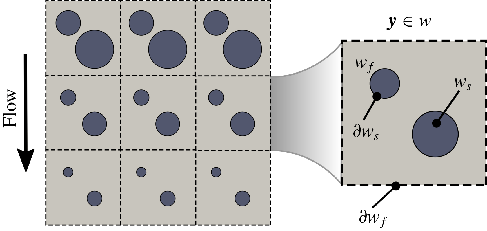
Contaminant adsorption occurs at different rates in different unit cells, depending on the local particle concentration and flow. As a result, fibres in unit cells can grow differently (see the schematic on the left of figure 1). However, we assume that the variations in diameter of the periodic fibres are small between adjacent unit cells, so that our microstructure is near-periodic and these variations are captured at the macroscale (see more discussions in Dalwadi et al. (Reference Dalwadi, Bruna and Griffiths2016)).

Figure 1. Microscale representation of the filter medium on the left and notations for the microscale quasi-periodic unit cell
 $w$
with a microscale variable
$w$
with a microscale variable
 $\boldsymbol{y}=\boldsymbol{x}/\unicode[STIX]{x1D6FF}$
varying in
$\boldsymbol{y}=\boldsymbol{x}/\unicode[STIX]{x1D6FF}$
varying in
 $w$
on the right.
$w$
on the right.
We suppose that the medium is composed of unidirectional fibres, which naturally reduces the model to a two-dimensional (2D) microstructure (see figure 2), though we note that all of the analysis presented here readily extends to the three-dimensional (3D) case.
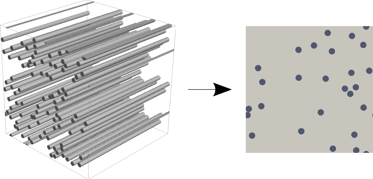
Figure 2. Non-woven filter-medium microstructure with unidirectional fibres: 3D and 2D representations on the left and right, respectively.
The macroscopic domain is denoted
 $\tilde{\unicode[STIX]{x1D6FA}}\subset \mathbb{R}^{2}$
and consists of the fluid and solid subdomains
$\tilde{\unicode[STIX]{x1D6FA}}\subset \mathbb{R}^{2}$
and consists of the fluid and solid subdomains
 $\tilde{\unicode[STIX]{x1D6FA}}_{f}(\tilde{t})$
and
$\tilde{\unicode[STIX]{x1D6FA}}_{f}(\tilde{t})$
and
 $\tilde{\unicode[STIX]{x1D6FA}}_{s}(\tilde{t})$
, respectively, where tildes denote dimensional quantities. The solid subdomain
$\tilde{\unicode[STIX]{x1D6FA}}_{s}(\tilde{t})$
, respectively, where tildes denote dimensional quantities. The solid subdomain
 $\tilde{\unicode[STIX]{x1D6FA}}_{s}$
represents the fibres. The interface between the subdomains is denoted
$\tilde{\unicode[STIX]{x1D6FA}}_{s}$
represents the fibres. The interface between the subdomains is denoted
 $\unicode[STIX]{x2202}\tilde{\unicode[STIX]{x1D6FA}}_{s}(\tilde{t})=\tilde{\unicode[STIX]{x1D6FA}}_{f}\cap \tilde{\unicode[STIX]{x1D6FA}}_{s}$
and represents the total surface of the fibres. We note that both subdomains depend on time
$\unicode[STIX]{x2202}\tilde{\unicode[STIX]{x1D6FA}}_{s}(\tilde{t})=\tilde{\unicode[STIX]{x1D6FA}}_{f}\cap \tilde{\unicode[STIX]{x1D6FA}}_{s}$
and represents the total surface of the fibres. We note that both subdomains depend on time
 $\tilde{t}$
due to fibre growth.
$\tilde{t}$
due to fibre growth.
2.1 Microstructure with isolated fibres
First, we consider the case when fibres are not allowed to touch at any time
 $\tilde{t}$
. We recall that this was the assumption used by Dalwadi et al. (Reference Dalwadi, Bruna and Griffiths2016), but here we extend it to polydisperse fibres. We define the domain by setting the location of the fibres in
$\tilde{t}$
. We recall that this was the assumption used by Dalwadi et al. (Reference Dalwadi, Bruna and Griffiths2016), but here we extend it to polydisperse fibres. We define the domain by setting the location of the fibres in
 $\tilde{\unicode[STIX]{x1D6FA}}(\tilde{t})$
with centres located at
$\tilde{\unicode[STIX]{x1D6FA}}(\tilde{t})$
with centres located at
 $\tilde{\boldsymbol{x}}^{m}$
and radii
$\tilde{\boldsymbol{x}}^{m}$
and radii
 $\tilde{r}^{m}(\tilde{\boldsymbol{x}},\tilde{t})$
for
$\tilde{r}^{m}(\tilde{\boldsymbol{x}},\tilde{t})$
for
 $m\in M$
, where
$m\in M$
, where
 $M$
is the set of all fibres in the whole filter medium, and prescribe
$M$
is the set of all fibres in the whole filter medium, and prescribe
 $\tilde{\unicode[STIX]{x1D6FA}}(\tilde{t}=0)$
. We denote the surface of each fibre as
$\tilde{\unicode[STIX]{x1D6FA}}(\tilde{t}=0)$
. We denote the surface of each fibre as
 $$\begin{eqnarray}\unicode[STIX]{x2202}\tilde{\unicode[STIX]{x1D6FA}}_{s}^{m}(\tilde{t})=\{\tilde{\boldsymbol{x}}\in \tilde{\unicode[STIX]{x1D6FA}}:\Vert \tilde{\boldsymbol{x}}-\tilde{\boldsymbol{x}}^{m}\Vert =\tilde{r}^{m}(\tilde{\boldsymbol{x}}^{m},\tilde{t})\},\quad m\in M.\end{eqnarray}$$
The interface between the pore and solid subdomains is the union of all the fibre surfaces, that is,
 $\unicode[STIX]{x2202}\tilde{\unicode[STIX]{x1D6FA}}_{s}(\tilde{t})=\bigcup _{m\in M}\unicode[STIX]{x2202}\tilde{\unicode[STIX]{x1D6FA}}_{s}^{m}(\tilde{t})$
. We note that the assumption that fibres are not in contact implies that
$\unicode[STIX]{x2202}\tilde{\unicode[STIX]{x1D6FA}}_{s}(\tilde{t})=\bigcup _{m\in M}\unicode[STIX]{x2202}\tilde{\unicode[STIX]{x1D6FA}}_{s}^{m}(\tilde{t})$
. We note that the assumption that fibres are not in contact implies that
 $\unicode[STIX]{x2202}\tilde{\unicode[STIX]{x1D6FA}}_{s}^{m}(\tilde{t})\cap \unicode[STIX]{x2202}\tilde{\unicode[STIX]{x1D6FA}}_{s}^{n}(\tilde{t})=\emptyset$
for
$\unicode[STIX]{x2202}\tilde{\unicode[STIX]{x1D6FA}}_{s}^{m}(\tilde{t})\cap \unicode[STIX]{x2202}\tilde{\unicode[STIX]{x1D6FA}}_{s}^{n}(\tilde{t})=\emptyset$
for
 $n\neq m$
.
$n\neq m$
.
The contaminant particles and the fluid occupy the pore space of the filter medium,
 $\tilde{\unicode[STIX]{x1D6FA}}_{f}(\tilde{t})$
. We assume that the particles are sufficiently small that they do not influence the fluid flow and that the flow is incompressible and Newtonian. We also assume that the flow is sufficiently slow and thus satisfies the Stokes equations
$\tilde{\unicode[STIX]{x1D6FA}}_{f}(\tilde{t})$
. We assume that the particles are sufficiently small that they do not influence the fluid flow and that the flow is incompressible and Newtonian. We also assume that the flow is sufficiently slow and thus satisfies the Stokes equations
 $$\begin{eqnarray}\displaystyle & -\tilde{\unicode[STIX]{x1D735}}\tilde{p}+\unicode[STIX]{x1D707}\tilde{\unicode[STIX]{x1D6FB}}^{2}\tilde{\boldsymbol{u}}=\mathbf{0},\quad \tilde{\boldsymbol{x}}\in \tilde{\unicode[STIX]{x1D6FA}}_{f}(\tilde{t}), & \displaystyle\end{eqnarray}$$
 $$\begin{eqnarray}\displaystyle & \hspace{36.0pt}\tilde{\unicode[STIX]{x1D735}}\boldsymbol{\cdot }\tilde{\boldsymbol{u}}=0,\quad \hspace{0.2pt}\tilde{\boldsymbol{x}}\in \tilde{\unicode[STIX]{x1D6FA}}_{f}(\tilde{t}), & \displaystyle\end{eqnarray}$$
where
 $\tilde{p}(\tilde{\boldsymbol{x}},\tilde{t})$
is the fluid pressure (Pa),
$\tilde{p}(\tilde{\boldsymbol{x}},\tilde{t})$
is the fluid pressure (Pa),
 $\tilde{\boldsymbol{u}}(\tilde{\boldsymbol{x}},\tilde{t})$
is the fluid velocity
$\tilde{\boldsymbol{u}}(\tilde{\boldsymbol{x}},\tilde{t})$
is the fluid velocity
 $(\text{m}~\text{s}^{-1})$
,
$(\text{m}~\text{s}^{-1})$
,
 $\tilde{\unicode[STIX]{x1D735}}$
is the nabla operator with respect to the spatial coordinate
$\tilde{\unicode[STIX]{x1D735}}$
is the nabla operator with respect to the spatial coordinate
 $\tilde{\boldsymbol{x}}$
, and
$\tilde{\boldsymbol{x}}$
, and
 $\unicode[STIX]{x1D707}$
is the viscosity (Pa s). The radial fibre growth results in the following no-slip boundary condition on the fibre surface:
$\unicode[STIX]{x1D707}$
is the viscosity (Pa s). The radial fibre growth results in the following no-slip boundary condition on the fibre surface:
 $$\begin{eqnarray}\tilde{\boldsymbol{u}}=-\frac{\unicode[STIX]{x2202}\tilde{r}^{m}}{\unicode[STIX]{x2202}\tilde{t}}\boldsymbol{n}^{m},\quad \tilde{\boldsymbol{x}}\in \unicode[STIX]{x2202}\tilde{\unicode[STIX]{x1D6FA}}_{s}^{m}(\tilde{t}),~m\in M,\end{eqnarray}$$
where
 $\boldsymbol{n}^{m}$
is the unit normal to the fibres’ surface
$\boldsymbol{n}^{m}$
is the unit normal to the fibres’ surface
 $\unicode[STIX]{x2202}\tilde{\unicode[STIX]{x1D6FA}}_{s}^{m}$
pointing into the solid domain. Despite the time-dependent nature of the boundary condition (2.2c
), we use the steady-state Stokes equations (2.2a
) and (2.2b
) because the time scale of fibre growth is slow compared with that over which the fluid flow attains a steady state.
$\unicode[STIX]{x2202}\tilde{\unicode[STIX]{x1D6FA}}_{s}^{m}$
pointing into the solid domain. Despite the time-dependent nature of the boundary condition (2.2c
), we use the steady-state Stokes equations (2.2a
) and (2.2b
) because the time scale of fibre growth is slow compared with that over which the fluid flow attains a steady state.
We assume that the contaminant particles are uniform in size. We also assume that they are much smaller than the typical fibre diameter and that the contaminant suspension is dilute, as is common for many filtration scenarios. This allows us to neglect particle–particle and hydrodynamic interactions and to describe the contaminant by its number concentration
 $\tilde{c}(\tilde{\boldsymbol{x}},\tilde{t})$
evolving according to
$\tilde{c}(\tilde{\boldsymbol{x}},\tilde{t})$
evolving according to
 $$\begin{eqnarray}\frac{\unicode[STIX]{x2202}\tilde{c}}{\unicode[STIX]{x2202}\tilde{t}}=\tilde{\unicode[STIX]{x1D735}}\boldsymbol{\cdot }(D\tilde{\unicode[STIX]{x1D735}}\tilde{c}-\tilde{\boldsymbol{u}}\tilde{c}),\quad \tilde{\boldsymbol{x}}\in \tilde{\unicode[STIX]{x1D6FA}}_{f}(\tilde{t}),\end{eqnarray}$$
where
 $\tilde{c}$
is measured in particle count
$\tilde{c}$
is measured in particle count
 $\text{m}^{-3}$
, and
$\text{m}^{-3}$
, and
 $D$
(
$D$
(
 $\text{m}^{2}~\text{s}^{-1}$
) is the diffusivity coefficient. Using a linear adsorption model without desorption (Baret Reference Baret1969) and (2.2c
), the boundary condition for the concentration reads
$\text{m}^{2}~\text{s}^{-1}$
) is the diffusivity coefficient. Using a linear adsorption model without desorption (Baret Reference Baret1969) and (2.2c
), the boundary condition for the concentration reads
 $$\begin{eqnarray}-D\tilde{\unicode[STIX]{x1D735}}\tilde{c}\boldsymbol{\cdot }\boldsymbol{n}^{m}=k\tilde{c},\quad \tilde{\boldsymbol{x}}\in \unicode[STIX]{x2202}\tilde{\unicode[STIX]{x1D6FA}}_{s}^{m}(\tilde{t}),~m\in M,\end{eqnarray}$$
where
 $k~(\text{m}~\text{s}^{-1})$
is the adsorption coefficient. For a detailed derivation of the boundary condition (2.4), we refer to Dalwadi et al. (Reference Dalwadi, Bruna and Griffiths2016). This represents a balance between the diffusive flux of particles to the fibre surface and the net adsorption as a result of contact, which, as discussed in the introduction (§ 1), may be due to a combination of mechanisms.
$k~(\text{m}~\text{s}^{-1})$
is the adsorption coefficient. For a detailed derivation of the boundary condition (2.4), we refer to Dalwadi et al. (Reference Dalwadi, Bruna and Griffiths2016). This represents a balance between the diffusive flux of particles to the fibre surface and the net adsorption as a result of contact, which, as discussed in the introduction (§ 1), may be due to a combination of mechanisms.
We assume that the contaminant particles become immobile once they adsorb onto the fibre surface and add to the fibre volume. Since we assume that the fibres grow radially, the radius of each fibre changes proportionally to the volumetric particle flux averaged over the surface of the fibre
 $\unicode[STIX]{x2202}\tilde{\unicode[STIX]{x1D6FA}}_{s}^{m}$
. This implies that
$\unicode[STIX]{x2202}\tilde{\unicode[STIX]{x1D6FA}}_{s}^{m}$
. This implies that
 $$\begin{eqnarray}\frac{\unicode[STIX]{x2202}\tilde{r}^{m}}{\unicode[STIX]{x2202}\tilde{t}}=\frac{1}{|\unicode[STIX]{x2202}\tilde{\unicode[STIX]{x1D6FA}}_{s}^{m}|}\int _{\unicode[STIX]{x2202}\tilde{\unicode[STIX]{x1D6FA}}_{s}^{m}}\unicode[STIX]{x1D70C}^{-1}v\,k\tilde{c}\,\text{d}s,\quad \tilde{\boldsymbol{x}}\in \unicode[STIX]{x2202}\tilde{\unicode[STIX]{x1D6FA}}_{s}^{m}(\tilde{t}),~m\in M,\end{eqnarray}$$
where
 $|\unicode[STIX]{x2202}\tilde{\unicode[STIX]{x1D6FA}}_{s}^{m}|=\int _{\unicode[STIX]{x2202}\tilde{\unicode[STIX]{x1D6FA}}_{s}^{m}}\,\text{d}s$
,
$|\unicode[STIX]{x2202}\tilde{\unicode[STIX]{x1D6FA}}_{s}^{m}|=\int _{\unicode[STIX]{x2202}\tilde{\unicode[STIX]{x1D6FA}}_{s}^{m}}\,\text{d}s$
,
 $v$
(
$v$
(
 $\text{m}^{3}$
) is the volume of a contaminant particle, and
$\text{m}^{3}$
) is the volume of a contaminant particle, and
 $\unicode[STIX]{x1D70C}$
is the packing density of contaminant particles on the fibre surface. If we ignore voids between the contaminant particles adsorbed onto the fibre surface, then
$\unicode[STIX]{x1D70C}$
is the packing density of contaminant particles on the fibre surface. If we ignore voids between the contaminant particles adsorbed onto the fibre surface, then
 $\unicode[STIX]{x1D70C}=1$
; if they are perfectly packed around the fibre, then
$\unicode[STIX]{x1D70C}=1$
; if they are perfectly packed around the fibre, then
 $\unicode[STIX]{x1D70C}=0.74$
. Generally, the particles do not pack so well and form so-called dendrites, or very dense tree-like structures (Brown Reference Brown1993, pp. 201–205). We consider
$\unicode[STIX]{x1D70C}=0.74$
. Generally, the particles do not pack so well and form so-called dendrites, or very dense tree-like structures (Brown Reference Brown1993, pp. 201–205). We consider
 $\unicode[STIX]{x1D70C}=0.3$
in this study.
$\unicode[STIX]{x1D70C}=0.3$
in this study.
2.1.1 Non-dimensionalization
We introduce the following non-dimensionalization:
where
 $l$
is the characteristic thickness of the filter medium (m),
$l$
is the characteristic thickness of the filter medium (m),
 ${\mathcal{U}}$
is the characteristic face velocity
${\mathcal{U}}$
is the characteristic face velocity
 $(\text{m}~\text{s}^{-1})$
,
$(\text{m}~\text{s}^{-1})$
,
 ${\mathcal{T}}$
is the characteristic filtration time (s), and
${\mathcal{T}}$
is the characteristic filtration time (s), and
 ${\mathcal{C}}$
is the inlet contaminant concentration (particle count
${\mathcal{C}}$
is the inlet contaminant concentration (particle count
 $\text{m}^{-3}$
). Here
$\text{m}^{-3}$
). Here
 $\unicode[STIX]{x1D6FF}$
is the ratio of the microscopic quasi-periodic unit-cell diameter to the (macroscopic) filter depth. The assumption to apply the method of multiple scales is that there is a separation between the microscopic and macroscopic length scales, that is,
$\unicode[STIX]{x1D6FF}$
is the ratio of the microscopic quasi-periodic unit-cell diameter to the (macroscopic) filter depth. The assumption to apply the method of multiple scales is that there is a separation between the microscopic and macroscopic length scales, that is,
 $\unicode[STIX]{x1D6FF}\ll 1$
.
$\unicode[STIX]{x1D6FF}\ll 1$
.
We also introduce the following dimensionless groups:
 $$\begin{eqnarray}\unicode[STIX]{x1D6FC}=\frac{l}{{\mathcal{U}}{\mathcal{T}}},\quad \unicode[STIX]{x1D6FD}=\frac{l\unicode[STIX]{x1D6FF}}{k{\mathcal{T}}},\quad \unicode[STIX]{x1D6FE}=\frac{D\unicode[STIX]{x1D6FF}}{lk},\quad \unicode[STIX]{x1D701}=\frac{{\mathcal{U}}\unicode[STIX]{x1D6FF}}{k},\quad \unicode[STIX]{x1D702}=\frac{{\mathcal{T}}v{\mathcal{C}}k}{\unicode[STIX]{x1D70C}\unicode[STIX]{x1D6FF}l},\end{eqnarray}$$
and the dimensionless domains
 $\unicode[STIX]{x1D6FA}$
,
$\unicode[STIX]{x1D6FA}$
,
 $\unicode[STIX]{x1D6FA}_{f}$
and
$\unicode[STIX]{x1D6FA}_{f}$
and
 $\unicode[STIX]{x2202}\unicode[STIX]{x1D6FA}_{s}^{m}$
, analogous to their dimensional counterparts. Inserting this non-dimensionalization into (2.2) yields
$\unicode[STIX]{x2202}\unicode[STIX]{x1D6FA}_{s}^{m}$
, analogous to their dimensional counterparts. Inserting this non-dimensionalization into (2.2) yields
 $$\begin{eqnarray}\displaystyle -\unicode[STIX]{x1D735}p+\unicode[STIX]{x1D6FF}^{2}\unicode[STIX]{x1D6FB}^{2}\boldsymbol{u} & = & \displaystyle \mathbf{0},\quad \hspace{44.39996pt}\boldsymbol{x}\in \unicode[STIX]{x1D6FA}_{f}(t),\end{eqnarray}$$
 $$\begin{eqnarray}\displaystyle \unicode[STIX]{x1D735}\boldsymbol{\cdot }\boldsymbol{u} & = & \displaystyle 0,\quad \hspace{44.39996pt}\boldsymbol{x}\in \unicode[STIX]{x1D6FA}_{f}(t),\end{eqnarray}$$
 $$\begin{eqnarray}\displaystyle \displaystyle \boldsymbol{u} & = & \displaystyle -\unicode[STIX]{x1D6FF}\unicode[STIX]{x1D6FC}\frac{\unicode[STIX]{x2202}r^{m}}{\unicode[STIX]{x2202}t}\boldsymbol{n}^{m},\quad \boldsymbol{x}\in \unicode[STIX]{x2202}\unicode[STIX]{x1D6FA}_{s}^{m}(t),~m\in M.\end{eqnarray}$$
 $$\begin{eqnarray}\displaystyle \displaystyle \unicode[STIX]{x1D6FD}\frac{\unicode[STIX]{x2202}c}{\unicode[STIX]{x2202}t}=\unicode[STIX]{x1D735}\boldsymbol{\cdot }(\unicode[STIX]{x1D6FE}\unicode[STIX]{x1D735}c-\unicode[STIX]{x1D701}\boldsymbol{u}c), & & \displaystyle \boldsymbol{x}\in \unicode[STIX]{x1D6FA}_{f}(t),\end{eqnarray}$$
 $$\begin{eqnarray}\displaystyle \unicode[STIX]{x1D6FE}\unicode[STIX]{x1D735}c\boldsymbol{\cdot }\boldsymbol{n}=-\unicode[STIX]{x1D6FF}c, & & \displaystyle \boldsymbol{x}\in \unicode[STIX]{x2202}\unicode[STIX]{x1D6FA}_{s}(t).\end{eqnarray}$$
 $$\begin{eqnarray}\frac{\unicode[STIX]{x2202}r^{m}}{\unicode[STIX]{x2202}t}=\frac{1}{|\unicode[STIX]{x2202}\unicode[STIX]{x1D6FA}_{s}^{m}|}\int _{\unicode[STIX]{x2202}\unicode[STIX]{x1D6FA}_{s}^{m}}\unicode[STIX]{x1D702}c\,\text{d}s,\quad m\in M.\end{eqnarray}$$
2.1.2 Homogenized model
At the microscale, we consider the filter medium to consist of quasi-periodic unit cells
 $w(\boldsymbol{x},t)$
(see figure 1). We allow for fibres of different sizes that may be randomly arranged within each periodic cell. We introduce a microscale variable
$w(\boldsymbol{x},t)$
(see figure 1). We allow for fibres of different sizes that may be randomly arranged within each periodic cell. We introduce a microscale variable
 $\boldsymbol{y}=\boldsymbol{x}/\unicode[STIX]{x1D6FF}$
, which is defined in the unit cell
$\boldsymbol{y}=\boldsymbol{x}/\unicode[STIX]{x1D6FF}$
, which is defined in the unit cell
 $w(\boldsymbol{x},t)$
. The macroscale variable
$w(\boldsymbol{x},t)$
. The macroscale variable
 $\boldsymbol{x}$
spans across the whole filter medium. We denote the fluid and solid subdomains as
$\boldsymbol{x}$
spans across the whole filter medium. We denote the fluid and solid subdomains as
 $w_{f}(\boldsymbol{x},t)$
and
$w_{f}(\boldsymbol{x},t)$
and
 $w_{s}(\boldsymbol{x},t)$
, respectively. The internal fluid–solid interface is denoted as
$w_{s}(\boldsymbol{x},t)$
, respectively. The internal fluid–solid interface is denoted as
 $\unicode[STIX]{x2202}w_{s}(\boldsymbol{x},t)$
, which consists of the fibre surfaces
$\unicode[STIX]{x2202}w_{s}(\boldsymbol{x},t)$
, which consists of the fibre surfaces
 $\unicode[STIX]{x2202}w_{s}(\boldsymbol{x},t)=\bigcup _{m\in M_{w}}\unicode[STIX]{x2202}w_{s}^{m}$
, where
$\unicode[STIX]{x2202}w_{s}(\boldsymbol{x},t)=\bigcup _{m\in M_{w}}\unicode[STIX]{x2202}w_{s}^{m}$
, where
 $M_{w}$
is the set of the fibres found in the unit cell, which is a subset of all fibres
$M_{w}$
is the set of the fibres found in the unit cell, which is a subset of all fibres
 $M$
in the filter medium,
$M$
in the filter medium,
 $M_{w}\subset M$
. The outer fluid boundary of the unit cell is denoted
$M_{w}\subset M$
. The outer fluid boundary of the unit cell is denoted
 $\unicode[STIX]{x2202}w_{f}(\boldsymbol{x},t)=\unicode[STIX]{x2202}w\cap w_{f}$
.
$\unicode[STIX]{x2202}w_{f}(\boldsymbol{x},t)=\unicode[STIX]{x2202}w\cap w_{f}$
.
Using the method of multiple scales, we seek a solution to the problem (2.8)–(2.10) as a function of
 $\boldsymbol{x}$
and
$\boldsymbol{x}$
and
 $\boldsymbol{y}$
, and treat these two variables as independent. The extra freedom this gives is removed by enforcing that the solution is exactly periodic in
$\boldsymbol{y}$
, and treat these two variables as independent. The extra freedom this gives is removed by enforcing that the solution is exactly periodic in
 $\boldsymbol{y}$
; small variations from one unit cell to the next are thereby captured through the macroscale variable
$\boldsymbol{y}$
; small variations from one unit cell to the next are thereby captured through the macroscale variable
 $\boldsymbol{x}$
. We insert the change of variables
$\boldsymbol{x}$
. We insert the change of variables
 $\boldsymbol{y}=\boldsymbol{x}/\unicode[STIX]{x1D6FF}$
and expand all dependent variables in the form
$\boldsymbol{y}=\boldsymbol{x}/\unicode[STIX]{x1D6FF}$
and expand all dependent variables in the form
 $\boldsymbol{u}=\boldsymbol{u}^{(0)}+\unicode[STIX]{x1D6FF}\boldsymbol{u}^{(1)}+\cdots \,$
, and similarly for the pressure
$\boldsymbol{u}=\boldsymbol{u}^{(0)}+\unicode[STIX]{x1D6FF}\boldsymbol{u}^{(1)}+\cdots \,$
, and similarly for the pressure
 $p$
and the concentration
$p$
and the concentration
 $c$
.
$c$
.
The macroscopic quantities are introduced using the following averaging:
 $$\begin{eqnarray}\overline{G}(\boldsymbol{x},t,\cdot )=\frac{1}{|w(\boldsymbol{x},t)|}\int _{w_{f}}g(\boldsymbol{x},\boldsymbol{y},t,\cdot )\,\text{d}\boldsymbol{y}=\unicode[STIX]{x1D719}G(\boldsymbol{x},t,\cdot ),\end{eqnarray}$$
where
 $g(\boldsymbol{x},\boldsymbol{y},t)$
is a microscopic quantity,
$g(\boldsymbol{x},\boldsymbol{y},t)$
is a microscopic quantity,
 $\overline{G}(\boldsymbol{x},t)$
is its volumetric average,
$\overline{G}(\boldsymbol{x},t)$
is its volumetric average,
 $G(\boldsymbol{x},t)$
is its intrinsic average, and
$G(\boldsymbol{x},t)$
is its intrinsic average, and
 $\unicode[STIX]{x1D719}=|w_{f}|/|w|$
is the porosity.
$\unicode[STIX]{x1D719}=|w_{f}|/|w|$
is the porosity.
For our homogenization, we use the volumetric average for the velocity
 $\overline{\boldsymbol{U}}$
and the intrinsic average for the pressure
$\overline{\boldsymbol{U}}$
and the intrinsic average for the pressure
 $P$
and concentration
$P$
and concentration
 $C$
. The velocity
$C$
. The velocity
 $\overline{\boldsymbol{U}}$
is the Darcy velocity and should not be confused with the actual velocity of the fluid travelling through the pores.
$\overline{\boldsymbol{U}}$
is the Darcy velocity and should not be confused with the actual velocity of the fluid travelling through the pores.
The derivation of the homogenized model via the method of multiple scales is analogous to that presented by Dalwadi et al. (Reference Dalwadi, Bruna and Griffiths2016) for monodisperse fibres. The same methodology can be easily extended to fibres with polydisperse sizes in the unit cell, when the fibres do not touch. For this reason, here we just present the final homogenized model and refer the reader to Dalwadi et al. (Reference Dalwadi, Bruna and Griffiths2016) for the details. In what follows, we drop the superscript (0) that refers to the leading-order quantities in
 $\unicode[STIX]{x1D6FF}$
and simply write
$\unicode[STIX]{x1D6FF}$
and simply write
 $\overline{\boldsymbol{U}}^{(0)}\equiv \overline{\boldsymbol{U}}$
, and similarly for
$\overline{\boldsymbol{U}}^{(0)}\equiv \overline{\boldsymbol{U}}$
, and similarly for
 $P$
and
$P$
and
 $C$
.
$C$
.
The homogenization of the flow problem (2.8) leads to Darcy’s equation, which relates
 $\overline{\boldsymbol{U}}$
and
$\overline{\boldsymbol{U}}$
and
 $P$
in terms of the permeability tensor
$P$
in terms of the permeability tensor
 $\boldsymbol{{\mathcal{K}}}$
:
$\boldsymbol{{\mathcal{K}}}$
:
 $$\begin{eqnarray}\displaystyle \overline{\boldsymbol{U}}(\boldsymbol{x},t) & = & \displaystyle -\boldsymbol{{\mathcal{K}}}\unicode[STIX]{x1D735}_{\boldsymbol{x}}P,\end{eqnarray}$$
 $$\begin{eqnarray}\displaystyle \displaystyle \boldsymbol{{\mathcal{K}}}(\boldsymbol{x},t) & = & \displaystyle \frac{1}{|w|}\int _{w_{f}}\unicode[STIX]{x1D646}\,\text{d}\boldsymbol{y}.\end{eqnarray}$$
 $\unicode[STIX]{x1D646}$
is a matrix-valued function and together with a vector-valued function
$\unicode[STIX]{x1D646}$
is a matrix-valued function and together with a vector-valued function
 $\unicode[STIX]{x1D72B}$
they satisfy the following cell problem at each location
$\unicode[STIX]{x1D72B}$
they satisfy the following cell problem at each location
 $\boldsymbol{x}$
:
$\boldsymbol{x}$
:  $$\begin{eqnarray}\displaystyle \unicode[STIX]{x1D644}-\unicode[STIX]{x1D735}_{\boldsymbol{y}}\unicode[STIX]{x1D72B}+\unicode[STIX]{x1D6FB}_{\boldsymbol{y}}^{2} & & \displaystyle \,\hspace{-12.0pt}\unicode[STIX]{x1D646}=\mathbf{0},\phantom{\text{periodic}}\hspace{1.6pt}\quad \boldsymbol{y}\in w_{f}(\boldsymbol{x},t),\end{eqnarray}$$
 $$\begin{eqnarray}\displaystyle \unicode[STIX]{x1D735}_{\boldsymbol{y}}\boldsymbol{\cdot } & & \displaystyle \,\hspace{-12.0pt}\unicode[STIX]{x1D646}=0,\phantom{\text{periodic}}\hspace{1.6pt}\quad \boldsymbol{y}\in w_{f}(\boldsymbol{x},t),\end{eqnarray}$$
 $$\begin{eqnarray}\displaystyle & & \displaystyle \,\hspace{-12.0pt}\unicode[STIX]{x1D646}=\mathbf{0},\phantom{\text{periodic}}\hspace{1.6pt}\quad \boldsymbol{y}\in \unicode[STIX]{x2202}w_{s}(\boldsymbol{x},t),\end{eqnarray}$$
 $$\begin{eqnarray}\displaystyle & & \displaystyle \,\hspace{-12.0pt}\unicode[STIX]{x1D646},\unicode[STIX]{x1D72B}~\text{periodic},\quad \boldsymbol{y}\in \unicode[STIX]{x2202}w_{f}(\boldsymbol{x},t),\end{eqnarray}$$
 $\unicode[STIX]{x1D644}$
is the identity matrix. For isotropic filter media, the permeability tensor becomes a multiple of the identity, that is,
$\unicode[STIX]{x1D644}$
is the identity matrix. For isotropic filter media, the permeability tensor becomes a multiple of the identity, that is,
 $\boldsymbol{{\mathcal{K}}}={\mathcal{K}}\unicode[STIX]{x1D644}$
with
$\boldsymbol{{\mathcal{K}}}={\mathcal{K}}\unicode[STIX]{x1D644}$
with
 ${\mathcal{K}}$
being a scalar. The macroscopic analogue to the incompressibility condition (2.8b
) is
${\mathcal{K}}$
being a scalar. The macroscopic analogue to the incompressibility condition (2.8b
) is  $$\begin{eqnarray}\unicode[STIX]{x1D735}_{\boldsymbol{x}}\boldsymbol{\cdot }\overline{\boldsymbol{U}}=\frac{\unicode[STIX]{x1D6FC}}{|w|}\mathop{\sum }_{m\in M_{w}}\int _{\unicode[STIX]{x2202}w_{s}^{m}}\frac{\unicode[STIX]{x2202}r^{m}}{\unicode[STIX]{x2202}t}\,\text{d}s=\frac{\unicode[STIX]{x1D6FC}}{|w|}\mathop{\sum }_{m\in M_{w}}\frac{\unicode[STIX]{x2202}r^{m}}{\unicode[STIX]{x2202}t}(2\unicode[STIX]{x03C0}r^{m})=-\unicode[STIX]{x1D6FC}\frac{\unicode[STIX]{x2202}\unicode[STIX]{x1D719}}{\unicode[STIX]{x2202}t},\end{eqnarray}$$
where
 $\unicode[STIX]{x1D6FC}$
is given in (2.7).
$\unicode[STIX]{x1D6FC}$
is given in (2.7).
Under the multiple-scales transformation, the contaminant-transport equation (2.9) becomes
 $$\begin{eqnarray}\unicode[STIX]{x1D6FD}\frac{\unicode[STIX]{x2202}(\unicode[STIX]{x1D719}C)}{\unicode[STIX]{x2202}t}=\unicode[STIX]{x1D735}_{\boldsymbol{x}}\boldsymbol{\cdot }(\unicode[STIX]{x1D6FE}\unicode[STIX]{x1D719}\boldsymbol{{\mathcal{D}}}\unicode[STIX]{x1D735}_{\boldsymbol{x}}C-\unicode[STIX]{x1D701}\overline{\boldsymbol{U}}C)-{\mathcal{A}}C,\end{eqnarray}$$
where
 $\unicode[STIX]{x1D6FD}$
and
$\unicode[STIX]{x1D6FD}$
and
 $\unicode[STIX]{x1D6FE}$
are given in (2.7) and
$\unicode[STIX]{x1D6FE}$
are given in (2.7) and
 ${\mathcal{A}}$
is the effective surface area of the fibres, defined as
${\mathcal{A}}$
is the effective surface area of the fibres, defined as
 ${\mathcal{A}}=|\unicode[STIX]{x2202}w_{s}|/|w|$
(that is, the surface area per unit volume of the medium). The effective diffusion coefficient
${\mathcal{A}}=|\unicode[STIX]{x2202}w_{s}|/|w|$
(that is, the surface area per unit volume of the medium). The effective diffusion coefficient
 $\boldsymbol{{\mathcal{D}}}=\boldsymbol{{\mathcal{D}}}(\boldsymbol{x},t,q)$
is computed as
$\boldsymbol{{\mathcal{D}}}=\boldsymbol{{\mathcal{D}}}(\boldsymbol{x},t,q)$
is computed as
 $$\begin{eqnarray}\boldsymbol{{\mathcal{D}}}=\unicode[STIX]{x1D644}-\frac{1}{|w_{f}|}\int _{w_{f}}\unicode[STIX]{x1D645}_{\unicode[STIX]{x1D6E4}}^{\,\text{T}}\,\text{d}\boldsymbol{y},\end{eqnarray}$$
where
 $(\unicode[STIX]{x1D645}_{\unicode[STIX]{x1D6E4}}^{\,\text{T}})_{ij}=\unicode[STIX]{x2202}\unicode[STIX]{x1D6E4}_{j}/\unicode[STIX]{x2202}y_{i}$
is the transpose of the Jacobian matrix of the vector-valued function
$(\unicode[STIX]{x1D645}_{\unicode[STIX]{x1D6E4}}^{\,\text{T}})_{ij}=\unicode[STIX]{x2202}\unicode[STIX]{x1D6E4}_{j}/\unicode[STIX]{x2202}y_{i}$
is the transpose of the Jacobian matrix of the vector-valued function
 $\unicode[STIX]{x1D71E}$
. Its components
$\unicode[STIX]{x1D71E}$
. Its components
 $\unicode[STIX]{x1D6E4}_{i}$
satisfy the cell problem:
$\unicode[STIX]{x1D6E4}_{i}$
satisfy the cell problem:
 $$\begin{eqnarray}\displaystyle \unicode[STIX]{x1D6FB}_{\boldsymbol{y}}^{2}\unicode[STIX]{x1D6E4}_{i} & = & \displaystyle 0,\hspace{20.30002pt}\quad \boldsymbol{y}\in w_{f}(\boldsymbol{x},t),\end{eqnarray}$$
 $$\begin{eqnarray}\displaystyle \unicode[STIX]{x1D735}_{\boldsymbol{y}}\unicode[STIX]{x1D6E4}_{i}\boldsymbol{\cdot }\boldsymbol{n}_{\boldsymbol{y}}^{m} & = & \displaystyle (\boldsymbol{n}_{\boldsymbol{y}}^{m})_{i},\hspace{5.0pt}\quad \boldsymbol{y}\in \unicode[STIX]{x2202}w_{s}^{m}(\boldsymbol{x},t),~m\in M_{w},\end{eqnarray}$$
 $$\begin{eqnarray}\displaystyle & & \displaystyle \hspace{-21.60004pt}\unicode[STIX]{x1D6E4}_{i}\text{periodic},\quad \boldsymbol{y}\in \unicode[STIX]{x2202}w_{f}(\boldsymbol{x},t),\end{eqnarray}$$
 $(\boldsymbol{n}_{\boldsymbol{y}}^{m})_{i}$
are the components of
$(\boldsymbol{n}_{\boldsymbol{y}}^{m})_{i}$
are the components of
 $\boldsymbol{n}_{\boldsymbol{y}}^{m}$
. We note that, in an analogous fashion to the permeability, we have
$\boldsymbol{n}_{\boldsymbol{y}}^{m}$
. We note that, in an analogous fashion to the permeability, we have
 $\boldsymbol{{\mathcal{D}}}={\mathcal{D}}\unicode[STIX]{x1D644}$
for the case of isotropic filter media.
$\boldsymbol{{\mathcal{D}}}={\mathcal{D}}\unicode[STIX]{x1D644}$
for the case of isotropic filter media.Finally, we obtain the following macroscopic coupling condition from (2.10):
 $$\begin{eqnarray}\frac{\unicode[STIX]{x2202}r^{m}}{\unicode[STIX]{x2202}t}=\unicode[STIX]{x1D702}C,\quad m\in M_{w},\end{eqnarray}$$
where
 $\unicode[STIX]{x1D702}$
is given in (2.7). Multiplying the left-hand side of (2.18) by
$\unicode[STIX]{x1D702}$
is given in (2.7). Multiplying the left-hand side of (2.18) by
 $|\unicode[STIX]{x2202}w_{s}^{m}|/|w|$
and summing over all fibres in the unit cell, we obtain the following relation between the fibre radii and the macroscopic porosity:
$|\unicode[STIX]{x2202}w_{s}^{m}|/|w|$
and summing over all fibres in the unit cell, we obtain the following relation between the fibre radii and the macroscopic porosity:
 $$\begin{eqnarray}\mathop{\sum }_{m\in M_{w}}\frac{|\unicode[STIX]{x2202}w_{s}^{m}|}{|w|}\frac{\unicode[STIX]{x2202}r^{m}}{\unicode[STIX]{x2202}t}=\frac{1}{|w|}\frac{\unicode[STIX]{x2202}}{\unicode[STIX]{x2202}t}\left(\mathop{\sum }_{m\in M_{w}}\unicode[STIX]{x03C0}(r^{m})^{2}\right)=-\frac{\unicode[STIX]{x2202}\unicode[STIX]{x1D719}}{\unicode[STIX]{x2202}t}.\end{eqnarray}$$
Doing the same for the right-hand side of (2.18) and noticing that
 $\sum _{m\in M_{w}}|\unicode[STIX]{x2202}w_{s}^{m}|/|w|={\mathcal{A}}$
, from (2.18) and (2.19) we obtain
$\sum _{m\in M_{w}}|\unicode[STIX]{x2202}w_{s}^{m}|/|w|={\mathcal{A}}$
, from (2.18) and (2.19) we obtain
 $$\begin{eqnarray}\frac{\unicode[STIX]{x2202}\unicode[STIX]{x1D719}}{\unicode[STIX]{x2202}t}=-\unicode[STIX]{x1D702}{\mathcal{A}}C.\end{eqnarray}$$
The diffusion of contaminant particles has a twofold impact on the filtration process. First, it acts as a bulk transport mechanism of the contaminant particles, appearing in the dimensionless parameter
 $\unicode[STIX]{x1D6FE}$
. Second, it corresponds to the driving feature in the capture mechanism, expressed by (2.20). The molecular diffusion
$\unicode[STIX]{x1D6FE}$
. Second, it corresponds to the driving feature in the capture mechanism, expressed by (2.20). The molecular diffusion
 $D$
and correspondingly the dimensionless parameter
$D$
and correspondingly the dimensionless parameter
 $\unicode[STIX]{x1D6FE}$
scale as
$\unicode[STIX]{x1D6FE}$
scale as
 $q^{-1}$
, where
$q^{-1}$
, where
 $q$
is the size of the contaminant particles, while the diffusion component in the adsorption coefficient
$q$
is the size of the contaminant particles, while the diffusion component in the adsorption coefficient
 $k$
scales as
$k$
scales as
 $q^{-2/3}$
according to an empirical adsorption model from Baron & Willeke (Reference Baron and Willeke2001, pp. 205–210). This means that, as particle size increases, the molecular diffusion
$q^{-2/3}$
according to an empirical adsorption model from Baron & Willeke (Reference Baron and Willeke2001, pp. 205–210). This means that, as particle size increases, the molecular diffusion
 $D$
converges to zero faster than the diffusion effect in the adsorption. As a result, it is possible to have a filtration regime where the diffusion term in (2.15) is negligible but particle adsorption is still mostly driven by diffusion. This will be the case in our advection-only regime.
$D$
converges to zero faster than the diffusion effect in the adsorption. As a result, it is possible to have a filtration regime where the diffusion term in (2.15) is negligible but particle adsorption is still mostly driven by diffusion. This will be the case in our advection-only regime.
For the sake of clarity, in this study we shall assume that
 $\unicode[STIX]{x1D702}$
is constant for all filtration regimes and for all fibres, but recognize that in reality it may vary for different filtration regimes and fibres and may also change with time. If we wanted to allow for different adsorption coefficients for different fibre surfaces, we would need to derive the equations in terms of an effective adsorption coefficient instead of the effective surface area
$\unicode[STIX]{x1D702}$
is constant for all filtration regimes and for all fibres, but recognize that in reality it may vary for different filtration regimes and fibres and may also change with time. If we wanted to allow for different adsorption coefficients for different fibre surfaces, we would need to derive the equations in terms of an effective adsorption coefficient instead of the effective surface area
 ${\mathcal{A}}$
, but we do not consider this here.
${\mathcal{A}}$
, but we do not consider this here.
2.2 Microstructure with closely located fibres
In random microstructures, the distance between different fibres varies (see figure 2). As contaminants are being deposited and fibres are growing, fibres located close to one another come into contact and form an agglomerate, while other more distant fibres can continue growing individually. To account for this scenario, we introduce the following agglomeration algorithm. If, as fibres grow radially, two or more fibres come into contact, we replace them with one larger fibre located at the centre of mass of the original fibres and with cross-sectional area equal to the sum of the areas of the individual fibres (see scenario 1 in figure 3 for an illustrative example). When replacing two fibres with a single larger fibre, the resulting fibre may overlap with other fibres located nearby in the unit cell. In such an instance, we recursively replace the overlapping or closely located fibres until the resulting fibre becomes isolated (see scenario 2 in figure 3). Owing to the periodic boundary conditions on the unit cell, the agglomeration algorithm also accounts for the periodic images of fibres.
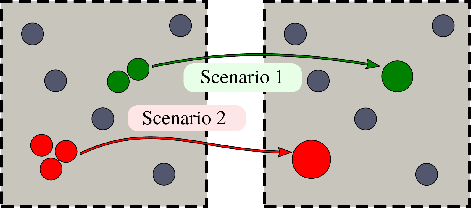
Figure 3. Agglomeration algorithm of touching fibres. Scenario 1: two fibres come into contact with one another at some point and are unified into a single fibre with the same volume with the same centre of mass. Scenario 2: two fibres come into contact with one another at some point and are unified into a single fibre which then overlaps with a neighbouring fibre. The unified fibre is then joined with the third fibre to form a fibre with the same volume and centre of mass as the three fibres.
The multiscale model of (2.12)–(2.17) and (2.20) is valid for any random and polydisperse configuration of fibres with different radii in the same unit cell. When, due to the fibre growth (2.18), two or more fibres come into contact, we perform the geometry transformation described above and then reapply the same model to the new geometry.
While this algorithm is clearly an idealization of the real process, it allows us to account for the formation of fibre agglomerates while keeping our strategy simple and robust. In the appendix we investigate the effect of the fibres coming into contact on the numerical simulations, in particular to confirm that the effective diffusivity
 $\boldsymbol{{\mathcal{D}}}$
converges to a limiting case.
$\boldsymbol{{\mathcal{D}}}$
converges to a limiting case.
The continuum assumption that was used to model the contaminant transport is violated as the distance between two fibres becomes comparable with the particle size. To resolve this issue, one can introduce into the agglomeration algorithm a critical distance between two fibres at which they coalesce to form an agglomerate, but we do not include this in our analysis here.
2.3 Multiscale algorithm
In this subsection, we describe the numerical implementation of the multiscale model. First, we perform the microscale simulations as a preprocessing step and find the effective parameters, namely, the permeability
 $\boldsymbol{{\mathcal{K}}}$
, the effective diffusivity
$\boldsymbol{{\mathcal{K}}}$
, the effective diffusivity
 $\boldsymbol{{\mathcal{D}}}$
and the effective surface area
$\boldsymbol{{\mathcal{D}}}$
and the effective surface area
 ${\mathcal{A}}$
, as functions of the porosity
${\mathcal{A}}$
, as functions of the porosity
 $\unicode[STIX]{x1D719}$
. The description of the microscale simulations is presented as a schematic algorithm in figure 4. As input parameters we specify the microstructure type, the initial porosity and the fibre diameter distribution. Using this input, we generate one unit cell in the case of regular microstructures (square or hexagonal), and perform Monte Carlo simulations using multiple random instances of unit cells in the case of random microstructures. Once the unit cell for the given porosity is characterized (with the parameters of interest listed above), we decrease the porosity by a small porosity step
$\unicode[STIX]{x1D719}$
. The description of the microscale simulations is presented as a schematic algorithm in figure 4. As input parameters we specify the microstructure type, the initial porosity and the fibre diameter distribution. Using this input, we generate one unit cell in the case of regular microstructures (square or hexagonal), and perform Monte Carlo simulations using multiple random instances of unit cells in the case of random microstructures. Once the unit cell for the given porosity is characterized (with the parameters of interest listed above), we decrease the porosity by a small porosity step
 $\unicode[STIX]{x0394}\unicode[STIX]{x1D719}$
. Then, we increase the fibre radii until the new porosity is reached and, if necessary, apply the agglomeration algorithm described in § 2.2. Finally, we compute the effective parameters corresponding to the updated porosity value. We continue this process until we have reconstructed the whole dependence of the effective parameters on the porosity (see, for example, figures 6 and 7). We note that, if we were to take a microstructure configuration obtained at a later time from this algorithm and run the process in reverse (increasing rather than decreasing porosity), then we would not recover the earlier configurations since we lose information about the original microstructure upon merging fibres. We could, however, create a different algorithm to describe a scenario in which the obstacles decrease in size and divide.
$\unicode[STIX]{x0394}\unicode[STIX]{x1D719}$
. Then, we increase the fibre radii until the new porosity is reached and, if necessary, apply the agglomeration algorithm described in § 2.2. Finally, we compute the effective parameters corresponding to the updated porosity value. We continue this process until we have reconstructed the whole dependence of the effective parameters on the porosity (see, for example, figures 6 and 7). We note that, if we were to take a microstructure configuration obtained at a later time from this algorithm and run the process in reverse (increasing rather than decreasing porosity), then we would not recover the earlier configurations since we lose information about the original microstructure upon merging fibres. We could, however, create a different algorithm to describe a scenario in which the obstacles decrease in size and divide.
As mentioned above and detailed in figure 4, in the case of random microstructures we need to perform Monte Carlo simulations using multiple samples of the unit cell for a given porosity value. Then, the resulting effective parameter
 $\boldsymbol{{\mathcal{P}}}\in \{\boldsymbol{{\mathcal{K}}},\boldsymbol{{\mathcal{D}}},{\mathcal{A}}\}$
is computed as an average over all samples. Our stopping criterion for the Monte Carlo algorithm reads
$\boldsymbol{{\mathcal{P}}}\in \{\boldsymbol{{\mathcal{K}}},\boldsymbol{{\mathcal{D}}},{\mathcal{A}}\}$
is computed as an average over all samples. Our stopping criterion for the Monte Carlo algorithm reads
 $$\begin{eqnarray}e_{MC}=\frac{e_{\boldsymbol{{\mathcal{P}}}}}{e_{\boldsymbol{{\mathcal{P}}}}+S_{\boldsymbol{{\mathcal{P}}}}}\leqslant \unicode[STIX]{x1D700},\end{eqnarray}$$
where
 $e_{MC}$
is the dimensionless Monte Carlo error,
$e_{MC}$
is the dimensionless Monte Carlo error,
 $\unicode[STIX]{x1D700}$
is the accuracy, and
$\unicode[STIX]{x1D700}$
is the accuracy, and
 $e_{\boldsymbol{{\mathcal{P}}}}$
and
$e_{\boldsymbol{{\mathcal{P}}}}$
and
 $S_{\boldsymbol{{\mathcal{P}}}}$
are computed as
$S_{\boldsymbol{{\mathcal{P}}}}$
are computed as
 $$\begin{eqnarray}e_{\boldsymbol{{\mathcal{P}}}}=\frac{1.96\displaystyle \mathop{\sum }_{i,j}\unicode[STIX]{x1D70E}_{{\mathcal{P}}_{ij}}}{\sqrt{N}},\quad S_{\boldsymbol{{\mathcal{P}}}}=\mathop{\sum }_{i,j}|E_{{\mathcal{P}}_{ij}}|.\end{eqnarray}$$
Here,
 ${\mathcal{P}}_{ij}$
is the effective surface area with
${\mathcal{P}}_{ij}$
is the effective surface area with
 $i,j=1$
or the components of the tensor
$i,j=1$
or the components of the tensor
 $\boldsymbol{{\mathcal{P}}}$
with
$\boldsymbol{{\mathcal{P}}}$
with
 $i,j=1,2$
in the case of the permeability or effective diffusivity and corresponds to the Monte Carlo samples
$i,j=1,2$
in the case of the permeability or effective diffusivity and corresponds to the Monte Carlo samples
 $w$
;
$w$
;
 $E_{{\mathcal{P}}_{ij}}$
and
$E_{{\mathcal{P}}_{ij}}$
and
 $\unicode[STIX]{x1D70E}_{{\mathcal{P}}_{ij}}$
are the mean and standard deviation of
$\unicode[STIX]{x1D70E}_{{\mathcal{P}}_{ij}}$
are the mean and standard deviation of
 ${\mathcal{P}}_{ij}$
, respectively, and
${\mathcal{P}}_{ij}$
, respectively, and
 $N$
is the number of Monte Carlo samples.
$N$
is the number of Monte Carlo samples.
We implement the microscopic algorithm in Python. We generate the unit cells and a triangular unstructured grid with refinement around the fibre surfaces using the open-source mesh generator GMSH (Geuzaine & Remacle Reference Geuzaine and Remacle2009). Then, we discretize the cell problems using the finite element library FEniCS (Alnæs et al.
Reference Alnæs, Blechta, Hake, Johansson, Kehlet, Logg, Richardson, Ring, Rognes and Wells2015) using linear Lagrange elements to solve (2.17) and a mixed finite element method to solve (2.13) with linear and quadratic Lagrange elements for
 $\unicode[STIX]{x1D72B}$
and
$\unicode[STIX]{x1D72B}$
and
 $\unicode[STIX]{x1D646}$
, respectively.
$\unicode[STIX]{x1D646}$
, respectively.
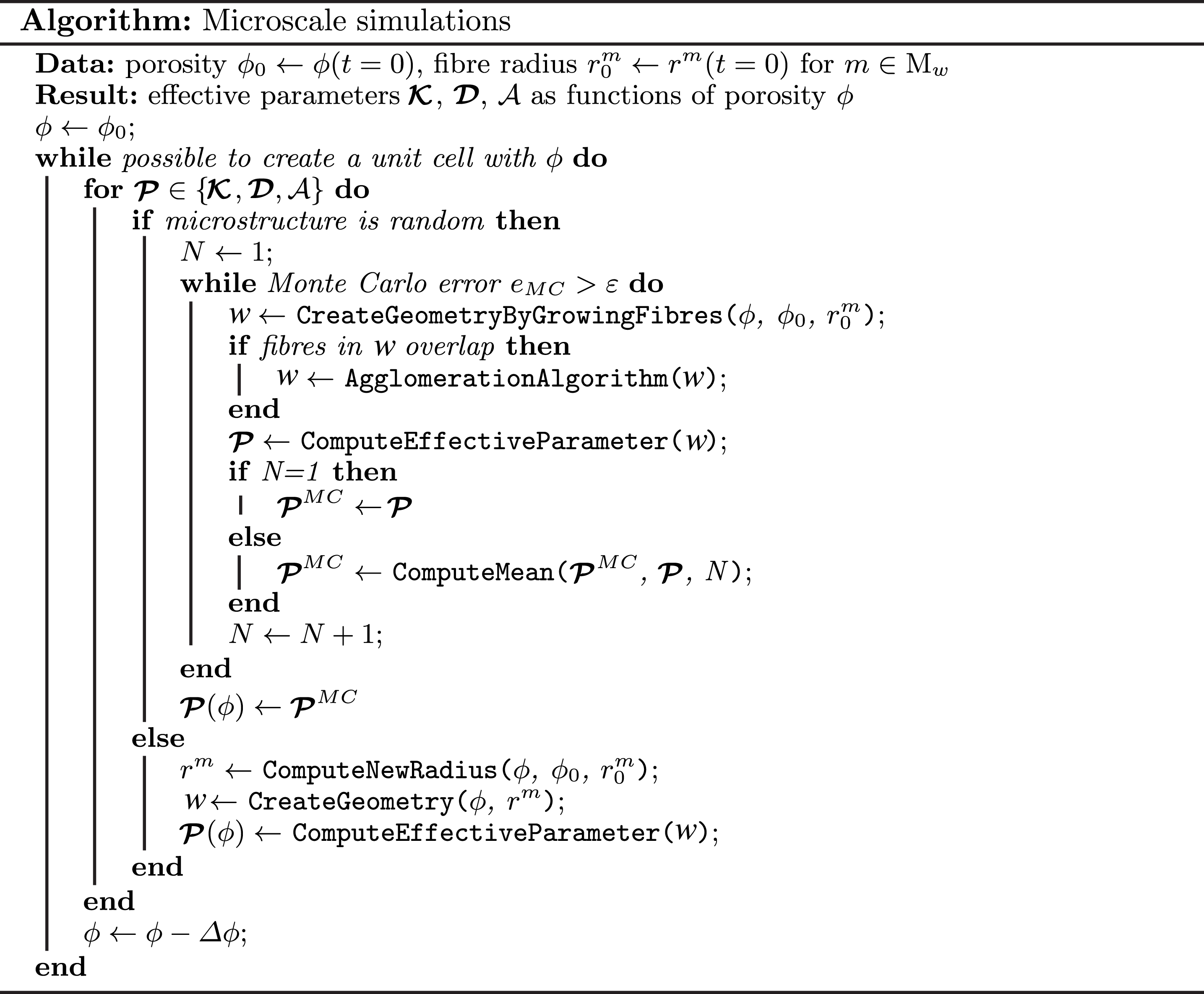
Figure 4. Algorithm for microscale simulations.
Once we know the dependences of the effective parameters on the porosity, we use them as coefficients in the macroscale model (2.12), (2.14), (2.15) and (2.20). The system of macroscale equations is also implemented in Python, discretizing time with an implicit backward Euler scheme and space finite elements from the FEniCS library using quadratic Lagrange elements for the pressure and linear Lagrange elements for all other variables. Starting with an initial guess, we find the solution iteratively in time. For a given time step, we solve the mass-conservation equation for the contaminant, equation (2.15), and the equation for the contaminant adsorption, equation (2.20), as a fully coupled nonlinear system using the Newton method. Then, we find the corresponding pressure and velocity distributions from (2.12) and (2.14) using the obtained porosity and proceed to the next time step.
3 Microscale simulations
In this section, we apply the microscale part of our homogenized model to quantify the three effective characteristics of different types of filter media: the permeability
 $\boldsymbol{{\mathcal{K}}}$
, the diffusivity
$\boldsymbol{{\mathcal{K}}}$
, the diffusivity
 $\boldsymbol{{\mathcal{D}}}$
and the surface area
$\boldsymbol{{\mathcal{D}}}$
and the surface area
 ${\mathcal{A}}$
. In particular, we consider five different microstructures, namely two regular and three random arrangements of fibres. The random microstructures are then extended periodically.
${\mathcal{A}}$
. In particular, we consider five different microstructures, namely two regular and three random arrangements of fibres. The random microstructures are then extended periodically.
We model non-woven filter media with an initial porosity
 $\unicode[STIX]{x1D719}(0)=0.93$
, which is a typical value for non-woven filter media used in air filters and purifiers – see, for example, table 1 in Das, Alagirusamy & Rajan Nagendra (Reference Das, Alagirusamy and Rajan Nagendra2009). To simulate the contaminant deposition, we employ the agglomeration algorithm discussed in § 2.2 to decrease the porosity
$\unicode[STIX]{x1D719}(0)=0.93$
, which is a typical value for non-woven filter media used in air filters and purifiers – see, for example, table 1 in Das, Alagirusamy & Rajan Nagendra (Reference Das, Alagirusamy and Rajan Nagendra2009). To simulate the contaminant deposition, we employ the agglomeration algorithm discussed in § 2.2 to decrease the porosity
 $\unicode[STIX]{x1D719}$
and to reconstruct the dependence of the effective parameters on the porosity
$\unicode[STIX]{x1D719}$
and to reconstruct the dependence of the effective parameters on the porosity
 $\unicode[STIX]{x1D719}$
.
$\unicode[STIX]{x1D719}$
.
As discussed in § 2, we model non-woven filter media using a unidirectional fibre arrangement, which enables a 2D representation of the microstructure (see figure 2). The choice of this representation was motivated by some preliminary validation carried out using experimental data and full 3D simulations using the commercial software package GeoDict (Math2Market GmbH 2011). The analysis showed that a 2D representation approximates well the permeability and the effective diffusivity of non-woven media with high porosity, while the effective surface area
 ${\mathcal{A}}$
is the same in the 2D case with unidirectional fibres and the 3D case with random orientation of fibres.
${\mathcal{A}}$
is the same in the 2D case with unidirectional fibres and the 3D case with random orientation of fibres.
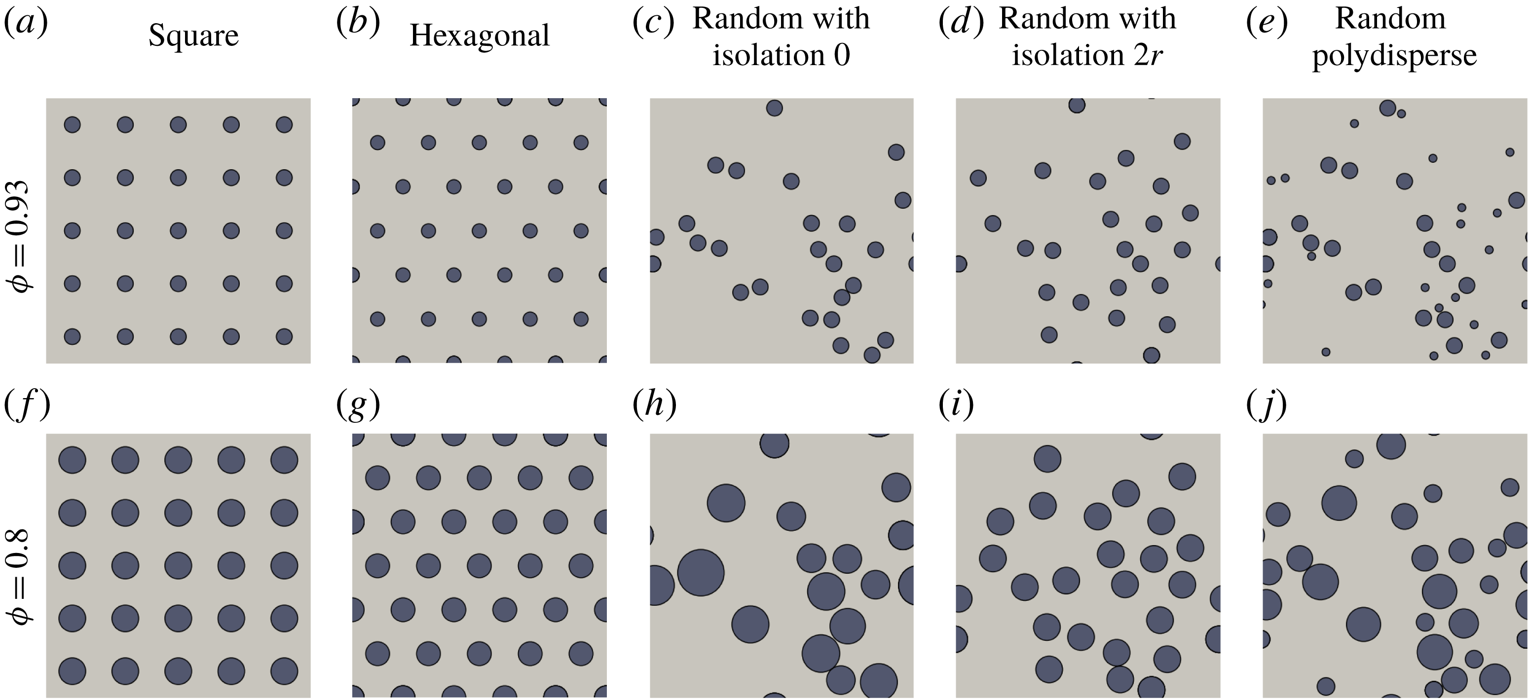
Figure 5(a–e) shows the five different microstructures corresponding to the clean filter media (before the contaminant deposition has begun). We note that, for the random microstructures, we show one random instance of the fibre distribution but that these will change from sample to sample. All microstructures have unidirectional fibres and differ by the distribution of the fibre centres and by the distribution of the fibre radii. The microstructures shown in figures 5(a,f), (b,g), (c,h) and (d,i) have fibres with monodisperse radii at
 $t=0$
, which are denoted
$t=0$
, which are denoted
 $r^{m}(\boldsymbol{x},0)=r$
constant for
$r^{m}(\boldsymbol{x},0)=r$
constant for
 $m\in M$
,
$m\in M$
,
 $\boldsymbol{x}\in \unicode[STIX]{x1D6FA}$
. The microstructure in figure 5(e, j) has polydisperse fibre radii and will be discussed in detail later.
$\boldsymbol{x}\in \unicode[STIX]{x1D6FA}$
. The microstructure in figure 5(e, j) has polydisperse fibre radii and will be discussed in detail later.

Figure 5. Different types of microstructures: square (a,f), hexagonal (b,g), random with mean isolation distances 0 (c,h) and
 $2r$
(d,i) and random with polydisperse fibre radii (e, j). (a–e) The microstructures when the filter media are clean, with the porosity
$2r$
(d,i) and random with polydisperse fibre radii (e, j). (a–e) The microstructures when the filter media are clean, with the porosity
 $\unicode[STIX]{x1D719}(0)=0.93$
. (f–j) The same microstructures after the simulations of fibre growth due to contaminant adsorption have been performed and the porosity
$\unicode[STIX]{x1D719}(0)=0.93$
. (f–j) The same microstructures after the simulations of fibre growth due to contaminant adsorption have been performed and the porosity
 $\unicode[STIX]{x1D719}=0.8$
is reached.
$\unicode[STIX]{x1D719}=0.8$
is reached.
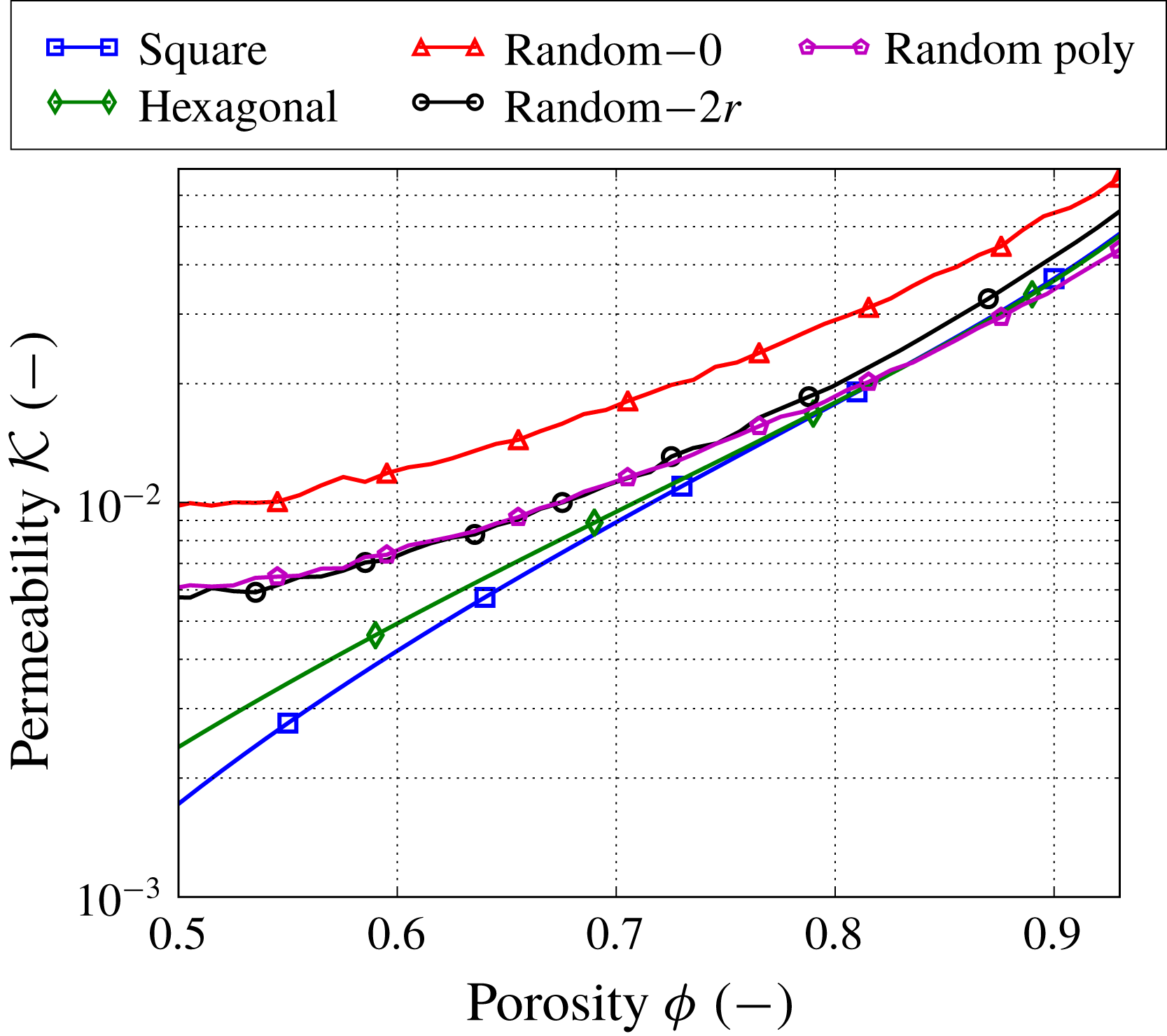
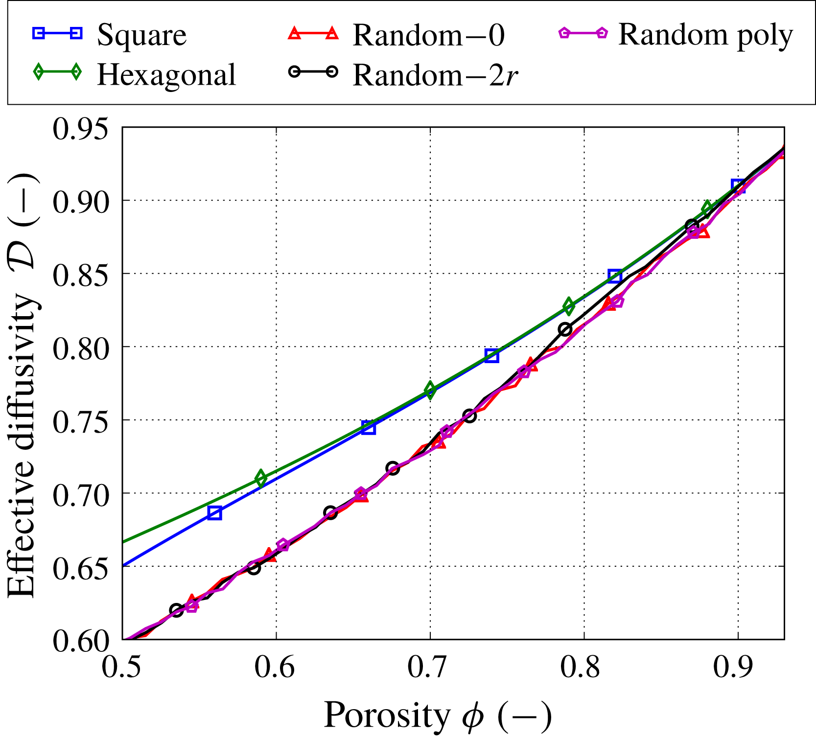
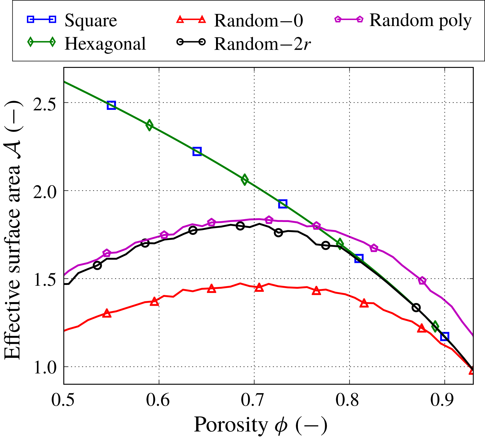
Figure 6. Permeability
 ${\mathcal{K}}$
as a function of porosity
${\mathcal{K}}$
as a function of porosity
 $\unicode[STIX]{x1D719}$
for different types of microstructures. The numbers next to the label ‘Random’ denote the mean isolation distance. For the random microstructures, the error bars are not shown, but fall within the markers’ size.
$\unicode[STIX]{x1D719}$
for different types of microstructures. The numbers next to the label ‘Random’ denote the mean isolation distance. For the random microstructures, the error bars are not shown, but fall within the markers’ size.
We consider regular microstructures with fibre centres located on square and hexagonal grids (see figures 5(a,f) and (b,g)). We then consider three types of random microstructures depending on the fibre position distribution and fibre diameter distribution. In all three cases, fibres are not allowed to overlap (if we try to place a fibre that overlaps, this is rejected and a new position is generated).
The first random microstructure has monodisperse fibre radii and fibre centres uniformly distributed in the unit cell. The problem with this structure is that it can result in areas with many fibres clustered together, and large gaps empty of fibres (see figure 5
c,h). Since this may not be very realistic for some filter media, in the second random microstructure, we impose an additional restriction to have some isolation distance around the fibres (see figure 5
d,i). While still considering fibres of constant physical radius
 $r$
, the idea is to introduce an average isolation distance so that we cover the unit cell in a more uniform manner. In particular, when placing a new fibre, we set an isolation distance
$r$
, the idea is to introduce an average isolation distance so that we cover the unit cell in a more uniform manner. In particular, when placing a new fibre, we set an isolation distance
 $d_{iso}$
, which is sampled from a log-normal distribution with mean
$d_{iso}$
, which is sampled from a log-normal distribution with mean
 $d$
and variance
$d$
and variance
 $d/3$
. Then, we attempt to place the new fibre, making sure that the distance between its centre and that of previously placed fibres is at least
$d/3$
. Then, we attempt to place the new fibre, making sure that the distance between its centre and that of previously placed fibres is at least
 $2r+d_{iso}$
(so note that, once a fibre is placed, we forget about its
$2r+d_{iso}$
(so note that, once a fibre is placed, we forget about its
 $d_{iso}$
). If not, we draw a new candidate position and a new isolation distance for the fibre and try again. The microstructure in figure 5(d,i) has mean isolation distance
$d_{iso}$
). If not, we draw a new candidate position and a new isolation distance for the fibre and try again. The microstructure in figure 5(d,i) has mean isolation distance
 $d=2r$
. The limiting case of the random microstructures with large isolation distance is the hexagonal model, which demonstrates that we can switch between regular and completely random microstructures by changing the isolation distance.
$d=2r$
. The limiting case of the random microstructures with large isolation distance is the hexagonal model, which demonstrates that we can switch between regular and completely random microstructures by changing the isolation distance.
The third random microstructure has uniformly distributed fibre centres with polydisperse fibre radii (see figure 5
e, j). We consider a random microstructure with two different fibre radii: 80 % volume-wise of the fibres have the same radius
 $r$
as before and the remaining 20 % are replaced with fibres with radius
$r$
as before and the remaining 20 % are replaced with fibres with radius
 $r/2$
. No isolation distance is imposed in this case, and the initial porosity is preserved to be
$r/2$
. No isolation distance is imposed in this case, and the initial porosity is preserved to be
 $\unicode[STIX]{x1D719}(0)=0.93$
.
$\unicode[STIX]{x1D719}(0)=0.93$
.
The second row in figure 5 shows the microstructures corresponding to the first row after fibres are grown to reach a porosity
 $\unicode[STIX]{x1D719}=0.8$
. The regular microstructures change only the fibre diameter, while in the random ones some agglomerates are formed. Microstructures with large mean isolation distance
$\unicode[STIX]{x1D719}=0.8$
. The regular microstructures change only the fibre diameter, while in the random ones some agglomerates are formed. Microstructures with large mean isolation distance
 $d$
(
$d$
(
 $d=2r$
in figure 5
d,i) yield fewer agglomerates as contaminants deposited on the fibres in comparison with the small
$d=2r$
in figure 5
d,i) yield fewer agglomerates as contaminants deposited on the fibres in comparison with the small
 $d$
(
$d$
(
 $d=0$
in figure 5
c,h). The microstructure with polydisperse fibre radii also leads to the formation of many agglomerates, but due to the presence of small fibres it preserves a more homogeneous structure during the lifetime of the medium than the microstructure with monodisperse fibres and no isolation distance.
$d=0$
in figure 5
c,h). The microstructure with polydisperse fibre radii also leads to the formation of many agglomerates, but due to the presence of small fibres it preserves a more homogeneous structure during the lifetime of the medium than the microstructure with monodisperse fibres and no isolation distance.
We perform microscale simulations for these five microstructure types to obtain the effective parameters, namely the permeability
 $\boldsymbol{{\mathcal{K}}}$
, the effective diffusivity
$\boldsymbol{{\mathcal{K}}}$
, the effective diffusivity
 $\boldsymbol{{\mathcal{D}}}$
and the effective area
$\boldsymbol{{\mathcal{D}}}$
and the effective area
 ${\mathcal{A}}$
, as functions of porosity
${\mathcal{A}}$
, as functions of porosity
 $\unicode[STIX]{x1D719}$
. Since all microstructures considered are isotropic, the permeability and effective diffusivity are presented as scalars, namely
$\unicode[STIX]{x1D719}$
. Since all microstructures considered are isotropic, the permeability and effective diffusivity are presented as scalars, namely
 $\boldsymbol{{\mathcal{K}}}\equiv {\mathcal{K}}\unicode[STIX]{x1D644}$
and
$\boldsymbol{{\mathcal{K}}}\equiv {\mathcal{K}}\unicode[STIX]{x1D644}$
and
 $\boldsymbol{{\mathcal{D}}}\equiv {\mathcal{D}}\unicode[STIX]{x1D644}$
(see § 2.1). For the random microstructures we perform Monte Carlo simulations to find the average effective parameters to an accuracy set to
$\boldsymbol{{\mathcal{D}}}\equiv {\mathcal{D}}\unicode[STIX]{x1D644}$
(see § 2.1). For the random microstructures we perform Monte Carlo simulations to find the average effective parameters to an accuracy set to
 $10^{-2}$
. Figures 6, 7 and 9 show the three effective parameters as functions of porosity. The error bars for the random microstructures are not shown, but they fall within the size of the markers.
$10^{-2}$
. Figures 6, 7 and 9 show the three effective parameters as functions of porosity. The error bars for the random microstructures are not shown, but they fall within the size of the markers.

Figure 7. The effective diffusivity
 ${\mathcal{D}}$
as a function of porosity
${\mathcal{D}}$
as a function of porosity
 $\unicode[STIX]{x1D719}$
for different types of microstructures. The numbers next to the label ‘Random’ denote the mean isolation distance. For the random microstructures, the error bars are not shown, but fall within the markers’ size.
$\unicode[STIX]{x1D719}$
for different types of microstructures. The numbers next to the label ‘Random’ denote the mean isolation distance. For the random microstructures, the error bars are not shown, but fall within the markers’ size.
The permeability
 ${\mathcal{K}}(\unicode[STIX]{x1D719})$
is computed using (2.12b
) after solving the cell problem (2.13). We observe that the permeability becomes more sensitive to the microstructure as the porosity decreases (figure 6). For example, the ratio between the maximum and minimum permeability values for the different microstructures is approximately 1.5 at
${\mathcal{K}}(\unicode[STIX]{x1D719})$
is computed using (2.12b
) after solving the cell problem (2.13). We observe that the permeability becomes more sensitive to the microstructure as the porosity decreases (figure 6). For example, the ratio between the maximum and minimum permeability values for the different microstructures is approximately 1.5 at
 $\unicode[STIX]{x1D719}=0.93$
and 5.7 at
$\unicode[STIX]{x1D719}=0.93$
and 5.7 at
 $\unicode[STIX]{x1D719}=0.5$
. Figure 8 shows the magnitude of vectors
$\unicode[STIX]{x1D719}=0.5$
. Figure 8 shows the magnitude of vectors
 $(\unicode[STIX]{x1D612}_{yx},\unicode[STIX]{x1D612}_{yy})$
, which are components of the matrix-valued function
$(\unicode[STIX]{x1D612}_{yx},\unicode[STIX]{x1D612}_{yy})$
, which are components of the matrix-valued function
 $\unicode[STIX]{x1D646}$
and correspond to the velocity profiles of the fluid flow in the vertical direction for different microstructures with porosity
$\unicode[STIX]{x1D646}$
and correspond to the velocity profiles of the fluid flow in the vertical direction for different microstructures with porosity
 $\unicode[STIX]{x1D719}=0.93$
. The flow profiles for the regular microstructures exhibit homogeneous behaviour for low velocities, while the flow profiles for the random microstructures allow for the development of high-velocity regions due to the presence of large empty spaces between the fibres. In this case, even with the same porosity, the random microstructures have higher average velocity than the regular ones and correspondingly larger permeability values. Among the random microstructures, the random case with zero isolation distance allows for the largest empty spaces. Increasing the isolation distance or adding fibre polydispersity both reduce the occurrence of large spaces, leading to more homogeneous velocity profiles.
$\unicode[STIX]{x1D719}=0.93$
. The flow profiles for the regular microstructures exhibit homogeneous behaviour for low velocities, while the flow profiles for the random microstructures allow for the development of high-velocity regions due to the presence of large empty spaces between the fibres. In this case, even with the same porosity, the random microstructures have higher average velocity than the regular ones and correspondingly larger permeability values. Among the random microstructures, the random case with zero isolation distance allows for the largest empty spaces. Increasing the isolation distance or adding fibre polydispersity both reduce the occurrence of large spaces, leading to more homogeneous velocity profiles.
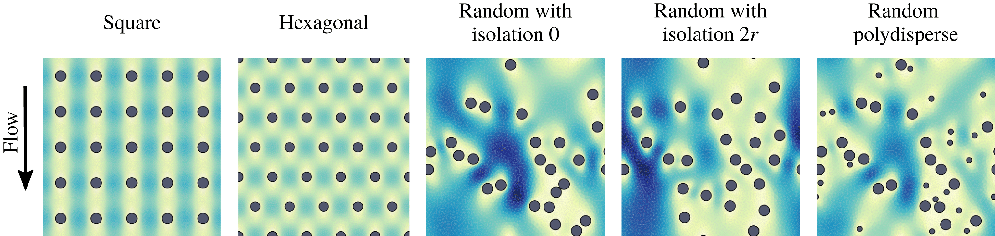
Figure 8. Magnitude of vectors
 $(\unicode[STIX]{x1D612}_{yx},\unicode[STIX]{x1D612}_{yy})$
for different types of microstructures with porosity
$(\unicode[STIX]{x1D612}_{yx},\unicode[STIX]{x1D612}_{yy})$
for different types of microstructures with porosity
 $\unicode[STIX]{x1D719}=0.93$
. Here
$\unicode[STIX]{x1D719}=0.93$
. Here
 $\unicode[STIX]{x1D612}_{yx}$
and
$\unicode[STIX]{x1D612}_{yx}$
and
 $\unicode[STIX]{x1D612}_{yy}$
are components of the matrix-valued function
$\unicode[STIX]{x1D612}_{yy}$
are components of the matrix-valued function
 $\unicode[STIX]{x1D646}$
and correspond to the velocity profiles in the vertical direction. All velocity profiles use the same maximum colour range exhibited by the random microstructure with no isolation distance.
$\unicode[STIX]{x1D646}$
and correspond to the velocity profiles in the vertical direction. All velocity profiles use the same maximum colour range exhibited by the random microstructure with no isolation distance.

Figure 9. Effective surface area
 ${\mathcal{A}}$
as a function of porosity
${\mathcal{A}}$
as a function of porosity
 $\unicode[STIX]{x1D719}$
for different types of microstructures. The numbers next to the label ‘Random’ denote the mean isolation distance. For the random microstructures, the error bars are not shown, but fall within the markers’ size.
$\unicode[STIX]{x1D719}$
for different types of microstructures. The numbers next to the label ‘Random’ denote the mean isolation distance. For the random microstructures, the error bars are not shown, but fall within the markers’ size.
The effective diffusivity
 ${\mathcal{D}}(\unicode[STIX]{x1D719})$
is computed using (2.16) after solving the cell problem (2.17). Figure 7 shows that all random microstructures have the same mean effective diffusivity, while the hexagonal and square microstructures provide slightly higher values. However, overall the effective diffusivity is less sensitive to different fibrous media than the permeability.
${\mathcal{D}}(\unicode[STIX]{x1D719})$
is computed using (2.16) after solving the cell problem (2.17). Figure 7 shows that all random microstructures have the same mean effective diffusivity, while the hexagonal and square microstructures provide slightly higher values. However, overall the effective diffusivity is less sensitive to different fibrous media than the permeability.
Finally, the effective surface area
 ${\mathcal{A}}(\unicode[STIX]{x1D719})$
is the same when the filter media are clean (
${\mathcal{A}}(\unicode[STIX]{x1D719})$
is the same when the filter media are clean (
 $\unicode[STIX]{x1D719}=0.93$
) for all microstructures except the one with polydisperse fibre radii, but it varies significantly as porosity decreases (figure 9). We also observe that the effective surface area of all random microstructures exhibits a non-monotonic behaviour. This happens due to the formation of agglomerates. As described in § 2.2, we preserve the cross-sectional area of the fibres when joining them in an agglomerate, which results in the reduction of their surface area. Similarly, as in real filtration, the surface area of an agglomerate is less than the total surface area of individual fibres forming the agglomerate and so the surface area available for further contaminant adsorption is reduced.
$\unicode[STIX]{x1D719}=0.93$
) for all microstructures except the one with polydisperse fibre radii, but it varies significantly as porosity decreases (figure 9). We also observe that the effective surface area of all random microstructures exhibits a non-monotonic behaviour. This happens due to the formation of agglomerates. As described in § 2.2, we preserve the cross-sectional area of the fibres when joining them in an agglomerate, which results in the reduction of their surface area. Similarly, as in real filtration, the surface area of an agglomerate is less than the total surface area of individual fibres forming the agglomerate and so the surface area available for further contaminant adsorption is reduced.
4 Methodology for macroscale simulations
In this section, we discuss several criteria to measure filter performance and present the operational regimes depending on the contaminant transport mechanism (advection, diffusion or both) and boundary conditions (filtration at constant pressure drop or constant inflow velocity).
Our macroscale homogenized model describes the filtration of contaminants in porous media, which is characterized by the three effective parameters: permeability, diffusivity and effective surface area. Earlier we assumed that the filter media have unidirectional fibres, which allowed us to describe the filtration problem using a 2D model with a spatial variable
 $\boldsymbol{x}=(x,y)$
. Now we also assume that the macroscale inflow velocity is purely one-dimensional (1D) in the direction of the depth of the filter, which we denote by
$\boldsymbol{x}=(x,y)$
. Now we also assume that the macroscale inflow velocity is purely one-dimensional (1D) in the direction of the depth of the filter, which we denote by
 $x$
, and takes the form
$x$
, and takes the form
 $\overline{\boldsymbol{U}}_{in}=(\overline{U}_{in},0)$
, and periodic boundary conditions in the transverse direction
$\overline{\boldsymbol{U}}_{in}=(\overline{U}_{in},0)$
, and periodic boundary conditions in the transverse direction
 $y$
. In addition, we assume the filter media have initially a constant porosity, that is, without macroscopic variations in its microstructure. As contaminant gets deposited in the fibres, the porosity will become a function of the depth
$y$
. In addition, we assume the filter media have initially a constant porosity, that is, without macroscopic variations in its microstructure. As contaminant gets deposited in the fibres, the porosity will become a function of the depth
 $x$
but remain independent of
$x$
but remain independent of
 $y$
. Then, the macroscopic problem is reduced to 1D with
$y$
. Then, the macroscopic problem is reduced to 1D with
 $\boldsymbol{x}\equiv x\in (0,1)$
. We denote the scalar velocity by
$\boldsymbol{x}\equiv x\in (0,1)$
. We denote the scalar velocity by
 $\overline{U}$
.
$\overline{U}$
.
We note that at the microscale individual simulations can lead to non-isotropic permeability and effective diffusivity tensors due to the finite size of the unit cells. However, we are concerned with averaged effective tensors obtained via Monte Carlo simulations for isotropic microstructures, which result in tensors with negligible off-diagonal elements and allows us to consider a 1D macroscale model.
4.1 Filter performance criteria
The performance of the filter media can be evaluated by different criteria. In this study we consider the following metrics.
(i) Energy consumption: a small pressure drop
 $\unicode[STIX]{x0394}P(t)=P(0,t)-P(1,t)$
across the filter medium ensures economic use of energy. The pressure drop is determined by the permeability of the filter medium and the flow velocity.
$\unicode[STIX]{x0394}P(t)=P(0,t)-P(1,t)$
across the filter medium ensures economic use of energy. The pressure drop is determined by the permeability of the filter medium and the flow velocity.(ii) Throughput: a high fluid velocity
$\overline{U}$
achieves large throughput of contaminated fluid across the filter medium. We use the fluid velocity at the inlet
$\overline{U}_{in}(t)=\overline{U}(0,t)$
.(iii) Efficiency: to quantify how efficient the filter medium is at trapping the contaminants, we define the number efficiency
$E$
as (4.1)where$$\begin{eqnarray}E(t)=1-\frac{J_{C}(1,t)}{J_{C}(0,t)},\quad \text{with}~J_{C}(x,t)=-\unicode[STIX]{x1D6FE}\unicode[STIX]{x1D719}{\mathcal{D}}\frac{\text{d}C}{\text{d}x}+\unicode[STIX]{x1D701}\overline{U}C,\end{eqnarray}$$
$J_{C}$
is the concentration flux.(iv) Dirt-holding capacity: this tells us how much contaminant the filter medium stores over time and, therefore, for how long it can be used. The dirt-holding capacity
$H$
is defined as follows: (4.2)$$\begin{eqnarray}H(t)=\unicode[STIX]{x1D70C}\int _{0}^{1}\unicode[STIX]{x1D719}(x,0)-\unicode[STIX]{x1D719}(x,t)\,\text{d}x.\end{eqnarray}$$
(v) Lifetime
$T>0$
: different termination criteria of the filtration process can be used. For example, in filtration with a constant flow rate, the filter medium can be considered completely loaded when a critical pressure drop is reached. On the other hand, in filtration under a constant pressure drop, the lifetime can be determined when the flow rate becomes too small. We choose a criterion that suits both filtration regimes, namely, we set the lifetime
$T$
as the time when a minimum porosity
$\unicode[STIX]{x1D719}_{min}=0.5$
is reached at any location of the filter medium.


To quantify the influence of the microstructure on the filtration performance, we introduce some sensitivity characteristics based on the performance criteria discussed above. First, we consider how sensitive the dirt-holding capacity
 $H$
is to the microstructure. We compute the relative maximum difference in the dirt-holding capacity while all filter media are in operation:
$H$
is to the microstructure. We compute the relative maximum difference in the dirt-holding capacity while all filter media are in operation:
 $$\begin{eqnarray}S_{H}=\frac{\max _{i,j=1,\ldots ,N}|H_{i}(T^{\ast })-H_{j}(T^{\ast })|}{\max _{i=1,\ldots ,N}H_{i}(T^{\ast })},\quad \text{where}~T^{\ast }=\min _{i=1,\ldots ,N}T_{i},\end{eqnarray}$$
where the subscripts denote characteristics corresponding to different microstructures and
 $N$
is the number of microstructures considered (
$N$
is the number of microstructures considered (
 $N=5$
for us). Second, we quantify the deviations of the pressure drop and the fluid velocity depending on the microstructure:
$N=5$
for us). Second, we quantify the deviations of the pressure drop and the fluid velocity depending on the microstructure:
 $$\begin{eqnarray}\{S_{\unicode[STIX]{x0394}P},S_{\overline{\boldsymbol{U}}}\}=1-\frac{\min _{i=1,\ldots ,N}|f_{i}(T_{i})-f_{i}(0)|}{\max _{i=1,\ldots ,N}|f_{i}(T_{i})-f_{i}(0)|},\quad \text{where}~f=\left\{\begin{array}{@{}ll@{}}\unicode[STIX]{x0394}P\quad & \text{for}~S_{\unicode[STIX]{x0394}P},\\ \overline{U}_{in}\quad & \text{for}~S_{\overline{\boldsymbol{U}}}.\end{array}\right.\end{eqnarray}$$
Finally, we introduce a sensitivity characteristic for the lifetime of the filter medium in the same way that we introduced it for the pressure drop deviation:
 $$\begin{eqnarray}S_{T}=1-\frac{\min _{i=1,\ldots ,N}T_{i}}{\max _{i=1,\ldots ,N}T_{i}}.\end{eqnarray}$$
We note that the sensitivity characteristics
 $S_{H}$
,
$S_{H}$
,
 $S_{\unicode[STIX]{x0394}P}$
,
$S_{\unicode[STIX]{x0394}P}$
,
 $S_{\overline{\boldsymbol{U}}}$
and
$S_{\overline{\boldsymbol{U}}}$
and
 $S_{T}$
take values in
$S_{T}$
take values in
 $[0,1]$
. When they are close to zero, the respective performance criterion, that is, the dirt-holding capacity, the pressure drop, the fluid velocity or the lifetime, is not sensitive to the microstructures. In contrast, a sensitivity characteristic close to one implies there is an important difference in the performance criteria between different microstructures.
$[0,1]$
. When they are close to zero, the respective performance criterion, that is, the dirt-holding capacity, the pressure drop, the fluid velocity or the lifetime, is not sensitive to the microstructures. In contrast, a sensitivity characteristic close to one implies there is an important difference in the performance criteria between different microstructures.
4.2 Advection–diffusion regime
Equation (2.15) describes the transport of contaminant by advection and diffusion. Typically for filtration regimes with advection, the time scale for the trapping of contaminant particles is much longer than the time scale for fluid to be advected through the filter medium. Therefore,
 $\unicode[STIX]{x1D6FD}\ll 1$
and the time derivative in the mass transport (2.15) can be neglected. Hence, we consider the steady state of (2.15) coupled with the contaminant adsorption (2.20). We supplement (2.15) with the following boundary conditions. At the inflow boundary
$\unicode[STIX]{x1D6FD}\ll 1$
and the time derivative in the mass transport (2.15) can be neglected. Hence, we consider the steady state of (2.15) coupled with the contaminant adsorption (2.20). We supplement (2.15) with the following boundary conditions. At the inflow boundary
 $x=0$
, we specify the contaminant flux
$x=0$
, we specify the contaminant flux
 $J_{in}=1$
. At the outflow boundary
$J_{in}=1$
. At the outflow boundary
 $x=1$
, we use zero Neumann boundary condition for the concentration. Mathematically this reads (see Dalwadi, Griffiths & Bruna Reference Dalwadi, Griffiths and Bruna2015):
$x=1$
, we use zero Neumann boundary condition for the concentration. Mathematically this reads (see Dalwadi, Griffiths & Bruna Reference Dalwadi, Griffiths and Bruna2015):
 $$\begin{eqnarray}\displaystyle & \displaystyle \left.\left(-\unicode[STIX]{x1D6FE}\unicode[STIX]{x1D719}{\mathcal{D}}\frac{\text{d}C}{\text{d}x}+\unicode[STIX]{x1D701}\overline{U}C\right)\right|_{x=0}=J_{in},\quad t\in [0,T], & \displaystyle\end{eqnarray}$$
 $$\begin{eqnarray}\displaystyle & \displaystyle \left.\frac{\text{d}C}{\text{d}x}\right|_{x=1}=0,\quad t\in [0,T]. & \displaystyle\end{eqnarray}$$
 $$\begin{eqnarray}\unicode[STIX]{x1D719}(x,0)=\unicode[STIX]{x1D719}_{0},\quad x\in (0,1).\end{eqnarray}$$
When
 $\unicode[STIX]{x1D6FD}\ll 1$
, we can rewrite (2.15) using (2.20) as follows:
$\unicode[STIX]{x1D6FD}\ll 1$
, we can rewrite (2.15) using (2.20) as follows:
 $$\begin{eqnarray}-\frac{\text{d}J_{C}}{\text{d}x}+\frac{1}{\unicode[STIX]{x1D702}}\frac{\unicode[STIX]{x2202}\unicode[STIX]{x1D719}}{\unicode[STIX]{x2202}t}=0.\end{eqnarray}$$
Using (4.6) and setting
 $J_{in}=1$
, we can integrate (4.8) over the filter depth and time to obtain:
$J_{in}=1$
, we can integrate (4.8) over the filter depth and time to obtain:
 $$\begin{eqnarray}H(t)=\unicode[STIX]{x1D70C}\unicode[STIX]{x1D702}\int _{0}^{t}E(s)\,\text{d}s.\end{eqnarray}$$
Hence, the dirt-holding capacity
 $H$
becomes a cumulative measure of the number efficiency
$H$
becomes a cumulative measure of the number efficiency
 $E$
in filtration regimes when
$E$
in filtration regimes when
 $\unicode[STIX]{x1D6FD}\ll 1$
and the boundary conditions (4.6) are used. For this reason, in what follows we mainly discuss the dirt-holding capacity
$\unicode[STIX]{x1D6FD}\ll 1$
and the boundary conditions (4.6) are used. For this reason, in what follows we mainly discuss the dirt-holding capacity
 $H$
and not the number efficiency
$H$
and not the number efficiency
 $E$
in all filtration regimes except in the diffusion-only regime.
$E$
in all filtration regimes except in the diffusion-only regime.
4.3 Advection regime
If diffusion is negligible in comparison to advection, we have that
 $\unicode[STIX]{x1D6FE}\ll 1$
in addition to
$\unicode[STIX]{x1D6FE}\ll 1$
in addition to
 $\unicode[STIX]{x1D6FD}\ll 1$
and the time derivative in (2.15) being negligible. We note that we must enforce
$\unicode[STIX]{x1D6FD}\ll 1$
and the time derivative in (2.15) being negligible. We note that we must enforce
 $\unicode[STIX]{x1D6FF}\ll \unicode[STIX]{x1D6FE}\ll 1$
for the asymptotic analysis that we perform on system (2.9) to hold. (The case when
$\unicode[STIX]{x1D6FF}\ll \unicode[STIX]{x1D6FE}\ll 1$
for the asymptotic analysis that we perform on system (2.9) to hold. (The case when
 $\unicode[STIX]{x1D6FE}$
and
$\unicode[STIX]{x1D6FE}$
and
 $\unicode[STIX]{x1D6FF}$
are of comparable orders leads to a different distinguished limit and resulting multiscale model, and this is the subject of a future study.) Then, the Robin boundary condition (4.6a
) reduces to a Dirichlet boundary condition. We solve (2.15) and (4.6a
) and find the concentration distribution as
$\unicode[STIX]{x1D6FF}$
are of comparable orders leads to a different distinguished limit and resulting multiscale model, and this is the subject of a future study.) Then, the Robin boundary condition (4.6a
) reduces to a Dirichlet boundary condition. We solve (2.15) and (4.6a
) and find the concentration distribution as
 $$\begin{eqnarray}C(x,t)=\frac{J_{in}}{\unicode[STIX]{x1D701}\overline{U}(x,t)}\exp \left(-\int _{0}^{x}\frac{{\mathcal{A}}(\unicode[STIX]{x1D719}(z,t))}{\unicode[STIX]{x1D701}\overline{U}(z,t)}\,\text{d}z\right).\end{eqnarray}$$
Thus, in the advection-only regime the model simplifies greatly. This is particularly useful for an extended parameter study, where the same problem must be solved many times for different sets of parameters.
4.4 Diffusion regime
When diffusion is the dominant transport mechanism of contaminants inside the filter, we neglect the advection (
 $\unicode[STIX]{x1D701}\ll 1$
) and keep all other terms in (2.15). We note that when the diffusion is important the time scale of the contaminant trapping can be comparable with the diffusive processes and so
$\unicode[STIX]{x1D701}\ll 1$
) and keep all other terms in (2.15). We note that when the diffusion is important the time scale of the contaminant trapping can be comparable with the diffusive processes and so
 $\unicode[STIX]{x1D6FD}$
may not necessarily be small.
$\unicode[STIX]{x1D6FD}$
may not necessarily be small.
To facilitate the diffusion transport of contaminants across a filter medium, a large difference in concentrations at the opposite sides of the medium has to be maintained, in contrast to when advection is present. To model this set-up mathematically, we specify Dirichlet boundary conditions for the concentration at both sides of the medium:
 $$\begin{eqnarray}C(0,t)=C_{in}=1,\quad C(1,t)=0,\quad t\in [0,T].\end{eqnarray}$$
We note that, in this regime, the contaminant transport (2.15) decouples from the fluid flow (2.12a ) and (2.14). Therefore, we do not solve the fluid flow problem in this regime.
4.5
$\overline{U}_{in}=\text{const.}$
regime

To specify the constant flow rate, we use the following boundary conditions for the macroscopic equations (2.12a ) and (2.14):
 $$\begin{eqnarray}\overline{U}(0,t)=\overline{U}_{in},\quad P(1,t)=0,\quad t\in [0,T].\end{eqnarray}$$
The parameter
 $\unicode[STIX]{x1D6FC}$
in (2.14) represents the ratio between the time scale of the fibre growth due to the contaminant deposition and the time scale of the fluid advection through the filter medium, which is usually very small. Using
$\unicode[STIX]{x1D6FC}$
in (2.14) represents the ratio between the time scale of the fibre growth due to the contaminant deposition and the time scale of the fluid advection through the filter medium, which is usually very small. Using
 $\unicode[STIX]{x1D6FC}\ll 1$
and (4.12a,b
), the solution of the 1D flow model (2.12a
) and (2.14) is given by
$\unicode[STIX]{x1D6FC}\ll 1$
and (4.12a,b
), the solution of the 1D flow model (2.12a
) and (2.14) is given by
 $$\begin{eqnarray}\displaystyle \overline{U}(x,t) & = & \displaystyle \overline{U}_{in},\hspace{45.96002pt}\quad x\in (0,1)~\text{and}~t\in [0,T],\end{eqnarray}$$
 $$\begin{eqnarray}\displaystyle \displaystyle P(x,t) & = & \displaystyle \int _{x}^{1}\frac{1}{{\mathcal{K}}(z,t)}\,\text{d}z,\quad x\in (0,1)~\text{and}~t\in [0,T].\end{eqnarray}$$
 ${\mathcal{K}}$
is used only to compute the pressure distribution and it does not affect the velocity, which is constant in space and time. Since the mass-transport problem is coupled with the flow problem only via the fluid velocity (see (2.15) and (2.20)),
${\mathcal{K}}$
is used only to compute the pressure distribution and it does not affect the velocity, which is constant in space and time. Since the mass-transport problem is coupled with the flow problem only via the fluid velocity (see (2.15) and (2.20)),
 ${\mathcal{K}}$
does not impact the mass transport and, as a result, the efficiency
${\mathcal{K}}$
does not impact the mass transport and, as a result, the efficiency
 $E$
in this operational regime.
$E$
in this operational regime.4.6
$\unicode[STIX]{x0394}P=\text{const.}$
regime

To model the filtration regime with a constant pressure drop, we use the following boundary conditions for the flow equations (2.12a ) and (2.14):
 $$\begin{eqnarray}P(0,t)=\unicode[STIX]{x0394}P,\quad P(1,t)=0,\quad t\in [0,T].\end{eqnarray}$$
In this case the solution of the 1D flow problem is
 $$\begin{eqnarray}\overline{U}(x,t)=\bar{{\mathcal{K}}}(t)\left(\unicode[STIX]{x0394}P+\int _{0}^{1}\frac{1}{{\mathcal{K}}(\unicode[STIX]{x1D719}(y,t))}\left(\unicode[STIX]{x1D6FC}\int _{0}^{y}\frac{\unicode[STIX]{x2202}\unicode[STIX]{x1D719}(z,t)}{\unicode[STIX]{x2202}t}\,\text{d}z\right)\text{d}y\right)-\unicode[STIX]{x1D6FC}\int _{0}^{x}\frac{\unicode[STIX]{x2202}\unicode[STIX]{x1D719}(y,t)}{\unicode[STIX]{x2202}t}\,\text{d}y,\end{eqnarray}$$
where
 $$\begin{eqnarray}\bar{{\mathcal{K}}}(t)=\left(\int _{0}^{1}\frac{1}{{\mathcal{K}}(\unicode[STIX]{x1D719}(y,t))}\,\text{d}y\right)^{-1}.\end{eqnarray}$$
Moreover, using again that
 $\unicode[STIX]{x1D6FC}\ll 1$
, we find
$\unicode[STIX]{x1D6FC}\ll 1$
, we find
 $$\begin{eqnarray}\overline{U}(x,t)=\bar{{\mathcal{K}}}(t)\unicode[STIX]{x0394}P,\quad x\in (0,1),~t\in [0,1].\end{eqnarray}$$
Therefore, in this regime we see that the permeability
 ${\mathcal{K}}$
has a direct impact on the fluid velocity and thus the efficiency.
${\mathcal{K}}$
has a direct impact on the fluid velocity and thus the efficiency.
5 Multiscale simulations
In this section we present simulations of our multiscale model using the five microstructure types from § 3 and the filtration regimes discussed in § 4. In particular, we consider three different scenarios for the transport of the contaminant, i.e. diffusive, advective or both. For the latter two, we distinguish between filtration processes performed under a constant flow rate
 $\overline{U}_{in}=\text{const.}$
or a constant pressure drop
$\overline{U}_{in}=\text{const.}$
or a constant pressure drop
 $\unicode[STIX]{x0394}P=\text{const.}$
(see a summary of each regime in table 1).
$\unicode[STIX]{x0394}P=\text{const.}$
(see a summary of each regime in table 1).

Figure 10. Lifetime
 $T$
as a function of the microstructure type for all filtration regimes.
$T$
as a function of the microstructure type for all filtration regimes.
Table 1. Dimensionless parameters for all filtration regimes.
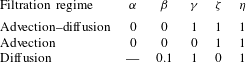
To maintain generality across the examples considered, we use the dimensionless model and, therefore, all parameters and results presented are also dimensionless. The input parameters are presented in table 2. Below we discuss the simulation results for each filtration regime in detail. A summary of the results is shown in table 3 in terms of the four sensitivity characteristics
 $S_{H},~S_{\unicode[STIX]{x0394}P},~S_{\overline{\boldsymbol{U}}}$
and
$S_{H},~S_{\unicode[STIX]{x0394}P},~S_{\overline{\boldsymbol{U}}}$
and
 $S_{T}$
and in figure 10 in terms of the lifetime values.
$S_{T}$
and in figure 10 in terms of the lifetime values.
Table 2. Input parameters for all numerical experiments.

Table 3. Characteristics of the microstructure sensitivity for all filtration regimes.
5.1 Advection–diffusion and
$\overline{U}_{in}=\text{const.}$
regime

The fluid flow is described by (4.13). The results of the numerical simulations for the five different microstructures are shown in figure 11(a–c). All microstructures exhibit similar filtration behaviour. The reduction of the pore space as contaminants are captured inside the filter medium results in the increase in contaminant capture and the number efficiency
 $E$
over time. Since we assume that the contaminants only adsorb and do not desorb, the dirt-holding capacity
$E$
over time. Since we assume that the contaminants only adsorb and do not desorb, the dirt-holding capacity
 $H$
is also an increasing function, which shows how much contaminant is stored in the filter medium at a given time
$H$
is also an increasing function, which shows how much contaminant is stored in the filter medium at a given time
 $t$
. The dirt-holding capacity
$t$
. The dirt-holding capacity
 $H$
at the lifetime
$H$
at the lifetime
 $T$
represents the maximum amount of contaminant that can be stored by this type of medium in this filtration regime.
$T$
represents the maximum amount of contaminant that can be stored by this type of medium in this filtration regime.
Regarding the different microstructures, we observe some variations in the number efficiency
 $E$
and the dirt-holding capacity
$E$
and the dirt-holding capacity
 $H$
in figures 11(a) and 11(b), respectively. The random microstructure with no isolation distance and monodisperse fibres has the lowest number efficiency of all the microstructures considered. On the other hand, the random microstructure with the polydisperse fibre radii shows the best number efficiency until
$H$
in figures 11(a) and 11(b), respectively. The random microstructure with no isolation distance and monodisperse fibres has the lowest number efficiency of all the microstructures considered. On the other hand, the random microstructure with the polydisperse fibre radii shows the best number efficiency until
 $t\approx 0.25$
, after which the regular microstructures exhibit the largest efficiency. Since the random microstructure with no isolation distance does not store as much contaminant as the other microstructures, it is not surprising that its lifetime is the longest (figure 10). However, overall the lifetime of a medium is not very sensitive to the microstructure: the sensitivity characteristic is
$t\approx 0.25$
, after which the regular microstructures exhibit the largest efficiency. Since the random microstructure with no isolation distance does not store as much contaminant as the other microstructures, it is not surprising that its lifetime is the longest (figure 10). However, overall the lifetime of a medium is not very sensitive to the microstructure: the sensitivity characteristic is
 $S_{T}=0.2$
(see table 3). The variations in the dirt-holding capacity
$S_{T}=0.2$
(see table 3). The variations in the dirt-holding capacity
 $H$
for the different microstructures (figure 11
b) are also small (
$H$
for the different microstructures (figure 11
b) are also small (
 $S_{H}=0.09$
). In contrast, the pressure drop
$S_{H}=0.09$
). In contrast, the pressure drop
 $\unicode[STIX]{x0394}P$
(figure 11
c) shows significant variations depending on the microstructure (
$\unicode[STIX]{x0394}P$
(figure 11
c) shows significant variations depending on the microstructure (
 $S_{\unicode[STIX]{x0394}P}=0.58$
). For example, the square grid microstructure reaches a pressure of approximately 160 at the end of the lifetime of the filter medium, while the random microstructure with zero isolation distance reaches only around 60 at the same time.
$S_{\unicode[STIX]{x0394}P}=0.58$
). For example, the square grid microstructure reaches a pressure of approximately 160 at the end of the lifetime of the filter medium, while the random microstructure with zero isolation distance reaches only around 60 at the same time.
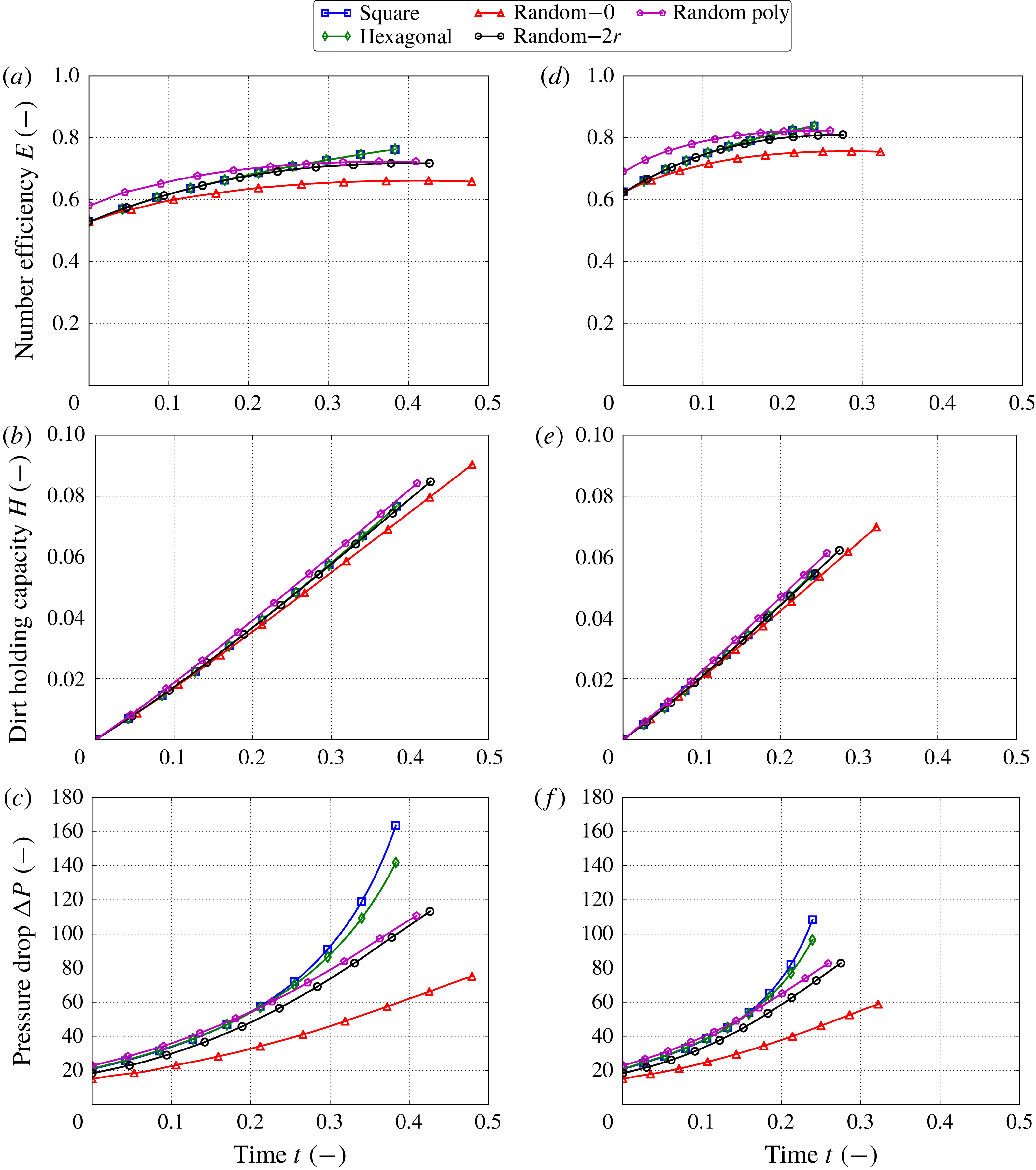
Figure 11. Multiscale simulation results for advection–diffusion (a–c) and for advection only (d–f), with
 $\overline{U}_{in}=\text{const.}$
We show the number efficiency
$\overline{U}_{in}=\text{const.}$
We show the number efficiency
 $E$
(a,d), the dirt-holding capacity
$E$
(a,d), the dirt-holding capacity
 $H$
(b,e) and the pressure drop
$H$
(b,e) and the pressure drop
 $\unicode[STIX]{x0394}P$
(c,f) as functions of time
$\unicode[STIX]{x0394}P$
(c,f) as functions of time
 $t$
.
$t$
.
5.2 Advection and
$\overline{U}_{in}=\text{const.}$
regime

Figure 11(d–f) shows the simulation results for the advection-only flow regime with constant flow rate for the different microstructures. The general filtration behaviour is the same as the previous filtration regime. We also observe that the dirt-holding capacity
 $H$
is not significantly influenced by the microstructure type (
$H$
is not significantly influenced by the microstructure type (
 $S_{H}=0.1$
, figure 11
e), while the pressure drop
$S_{H}=0.1$
, figure 11
e), while the pressure drop
 $\unicode[STIX]{x0394}P$
depends strongly on the microstructure model (
$\unicode[STIX]{x0394}P$
depends strongly on the microstructure model (
 $S_{\unicode[STIX]{x0394}P}=0.5$
, figure 11
f). The sensitivity of the lifetime of the filter media is
$S_{\unicode[STIX]{x0394}P}=0.5$
, figure 11
f). The sensitivity of the lifetime of the filter media is
 $S_{T}=0.26$
.
$S_{T}=0.26$
.
Comparing this regime with the advection–diffusion regime in § 5.1, we observe that the efficiency and dirt-holding capacity values are higher in the absence of the diffusive transport mechanism at any moment in time. This means that diffusion reduces the filtration efficacy for the same adsorption coefficient (see discussion in § 2.1.2 and further investigations in § 6). Nonetheless, the final dirt-holding capacity values are higher for the advection–diffusion regime than for the case of advection only when the filter media reach their lifetime. This means that the distribution of the dust within the filter depth improves in the presence of diffusion and the filter media can store more contaminants in total.
The pressure drop in the advection–diffusion regime is more sensitive to the different microstructure types than in the advection regime, while the dirt-holding capacity and the lifetime are slightly less sensitive to the microstructure. Overall, in these two filtration regimes with a constant flow rate, the permeability
 ${\mathcal{K}}$
significantly impacts the pressure drop, but does not influence the efficiency performance for the reasons discussed in § 4.5. In contrast, variations across microstructures in the effective diffusivity
${\mathcal{K}}$
significantly impacts the pressure drop, but does not influence the efficiency performance for the reasons discussed in § 4.5. In contrast, variations across microstructures in the effective diffusivity
 ${\mathcal{D}}$
and the effective surface area
${\mathcal{D}}$
and the effective surface area
 ${\mathcal{A}}$
have a small effect on the efficiency and dirt-holding capacity. For both filtration regimes, the random microstructure with the polydisperse fibre radii shows the best efficiency and dirt-holding capacity while having an average lifetime. Although this microstructure initially has the highest pressure drop, during the lifetime of the filter medium the pressure drop does not increase as rapidly as for the regular microstructures, and so when the filter reaches its lifetime the pressure drop is as low as that for the random microstructure with isolation distance
${\mathcal{A}}$
have a small effect on the efficiency and dirt-holding capacity. For both filtration regimes, the random microstructure with the polydisperse fibre radii shows the best efficiency and dirt-holding capacity while having an average lifetime. Although this microstructure initially has the highest pressure drop, during the lifetime of the filter medium the pressure drop does not increase as rapidly as for the regular microstructures, and so when the filter reaches its lifetime the pressure drop is as low as that for the random microstructure with isolation distance
 $2r$
.
$2r$
.
5.3 Advection–diffusion and
$\unicode[STIX]{x0394}P=\text{const.}$
regime

In this filtration regime, the fluid flow is determined by (4.17). Figure 12(a–c) shows the simulation results for the different microstructure models. Unlike the previous two regimes, here we hold the pressure drop constant, which results in the decrease of the throughput
 $\overline{U}_{in}$
over time. This happens because of the reduction of the pore space available for the fluid flow as the contaminants are being stored inside the filter medium. If we continued the simulations, the throughput would keep decreasing until it became zero when the filter medium was completely blocked by the contaminants.
$\overline{U}_{in}$
over time. This happens because of the reduction of the pore space available for the fluid flow as the contaminants are being stored inside the filter medium. If we continued the simulations, the throughput would keep decreasing until it became zero when the filter medium was completely blocked by the contaminants.
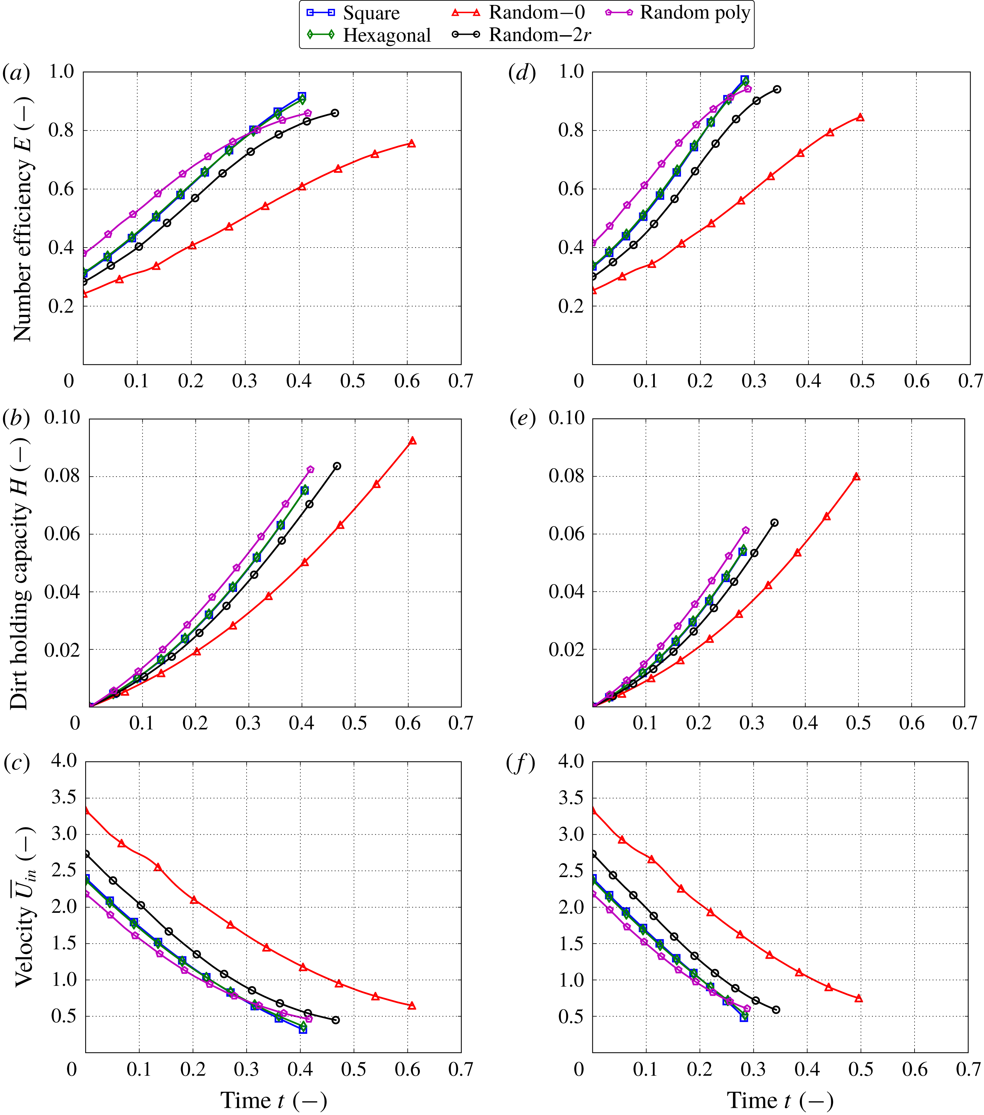
Figure 12. Multiscale simulation results for advection–diffusion (a–c) and for advection only (d–f), with
 $\unicode[STIX]{x0394}P=\text{const}$
. We show the number efficiency
$\unicode[STIX]{x0394}P=\text{const}$
. We show the number efficiency
 $E$
(a,d), the dirt-holding capacity
$E$
(a,d), the dirt-holding capacity
 $H$
(b,e) and the inflow velocity
$H$
(b,e) and the inflow velocity
 $\overline{U}_{in}$
(c,f) as functions of time
$\overline{U}_{in}$
(c,f) as functions of time
 $t$
.
$t$
.
The number efficiency
 $E$
and the dirt-holding capacity
$E$
and the dirt-holding capacity
 $H$
show strong dependences on the microstructure of the filter media in figures 12(a) and 12(b), respectively. The maximum difference in the dirt-holding capacity arises between the polydisperse random microstructure and the monodisperse random microstructure with no isolation distance, which have the best and worst dirt-holding capacity, respectively. The sensitivity of the dirt-holding capacity is characterized by
$H$
show strong dependences on the microstructure of the filter media in figures 12(a) and 12(b), respectively. The maximum difference in the dirt-holding capacity arises between the polydisperse random microstructure and the monodisperse random microstructure with no isolation distance, which have the best and worst dirt-holding capacity, respectively. The sensitivity of the dirt-holding capacity is characterized by
 $S_{H}=0.39$
. Again, the filter with the random microstructure with no isolation distance has a longer lifetime than all other microstructures because it does not store as much contaminant (figure 10). Overall, the lifetime of the filter media is quite sensitive to the microstructure (
$S_{H}=0.39$
. Again, the filter with the random microstructure with no isolation distance has a longer lifetime than all other microstructures because it does not store as much contaminant (figure 10). Overall, the lifetime of the filter media is quite sensitive to the microstructure (
 $S_{T}=0.33$
). Since the pressure drop is held constant during the filtration, the resulting pressure distribution for all microstructures is the same and is not shown here. Instead, we show the inflow velocity
$S_{T}=0.33$
). Since the pressure drop is held constant during the filtration, the resulting pressure distribution for all microstructures is the same and is not shown here. Instead, we show the inflow velocity
 $\overline{U}_{in}$
as a function of time in figure 12(c), which demonstrates the throughput of the fluid. The random microstructure with polydisperse fibre radii has the smallest throughput until around
$\overline{U}_{in}$
as a function of time in figure 12(c), which demonstrates the throughput of the fluid. The random microstructure with polydisperse fibre radii has the smallest throughput until around
 $t=0.3$
at which point it switches with the regular square and hexagonal microstructures. The random microstructure with no isolation distance demonstrates the largest throughput for all time. In general, the throughput is sensitive to the microstructure (
$t=0.3$
at which point it switches with the regular square and hexagonal microstructures. The random microstructure with no isolation distance demonstrates the largest throughput for all time. In general, the throughput is sensitive to the microstructure (
 $S_{\overline{\boldsymbol{U}}}=0.36$
).
$S_{\overline{\boldsymbol{U}}}=0.36$
).
5.4 Advection and
$\unicode[STIX]{x0394}P=\text{const.}$
regime

This regime is described by (4.10), (4.17) and (2.20). Figures 12(d) and 12(e) show that the number efficiency
 $E$
and the dirt-holding capacity
$E$
and the dirt-holding capacity
 $H$
are highly influenced by the microstructure. The sensitivity characteristic for the dirt-holding capacity is
$H$
are highly influenced by the microstructure. The sensitivity characteristic for the dirt-holding capacity is
 $S_{H}=0.48$
, the largest among the considered filtration regimes. Figure 10 shows the lifetime of the filter media, which varies between 0.28 for the random microstructure with polydisperse fibre radii and 0.5 for the random one with no isolation distance (
$S_{H}=0.48$
, the largest among the considered filtration regimes. Figure 10 shows the lifetime of the filter media, which varies between 0.28 for the random microstructure with polydisperse fibre radii and 0.5 for the random one with no isolation distance (
 $S_{T}=0.43$
). The throughput of the contaminated fluid has also a large sensitivity,
$S_{T}=0.43$
). The throughput of the contaminated fluid has also a large sensitivity,
 $S_{\overline{\boldsymbol{U}}}=0.39$
.
$S_{\overline{\boldsymbol{U}}}=0.39$
.
The filtration regimes when the pressure drop is held constant (this and previous subsection) experience a large increase in the efficiency during the lifetime of the filter. Moreover, these regimes are influenced significantly by the microstructure of the filter medium (see table 3). This implies that the effective parameters in (2.15) have a significant impact on the overall filtration. Comparing the two filtration regimes with the constant pressure drop, we observe that the advection regime is more sensitive to the microstructure than the advection–diffusion regime, which is similar to what we observed for the regimes with constant flow rate.
In both regimes with constant pressure drop, the random microstructure with the polydisperse fibre radii has the highest efficiency and dirt-holding capacity values. However, its lifetime and throughput are one of the lowest. On the other hand, the random microstructure with no isolation distance has the highest throughput but it captures few contaminants. Therefore, the best filter medium in these regimes is one with the random microstructure with isolation distance
 $2r$
that balances all the performance criteria. This medium offers good efficiency while providing the second largest throughput.
$2r$
that balances all the performance criteria. This medium offers good efficiency while providing the second largest throughput.
5.5 Diffusion regime
In this regime, we solve (2.15) and (2.20) with boundary conditions (4.11) and parameters specified in table 1. Figures 13(a) and 13(b) show the number efficiency
 $E$
and the dirt-holding capacity
$E$
and the dirt-holding capacity
 $H$
, respectively. Generally, for all microstructures, these characteristics follow the same trends as discussed earlier for the advection–diffusion and
$H$
, respectively. Generally, for all microstructures, these characteristics follow the same trends as discussed earlier for the advection–diffusion and
 $\overline{U}_{in}=\text{const.}$
filtration regime (see the first paragraph in § 5.1). Figure 10 shows the lifetime for all microstructure types, which varies between 0.24 and 0.32. The sensitivity characteristics for these two metrics are
$\overline{U}_{in}=\text{const.}$
filtration regime (see the first paragraph in § 5.1). Figure 10 shows the lifetime for all microstructure types, which varies between 0.24 and 0.32. The sensitivity characteristics for these two metrics are
 $S_{H}=0.17$
and
$S_{H}=0.17$
and
 $S_{T}=0.26$
(table 3).
$S_{T}=0.26$
(table 3).
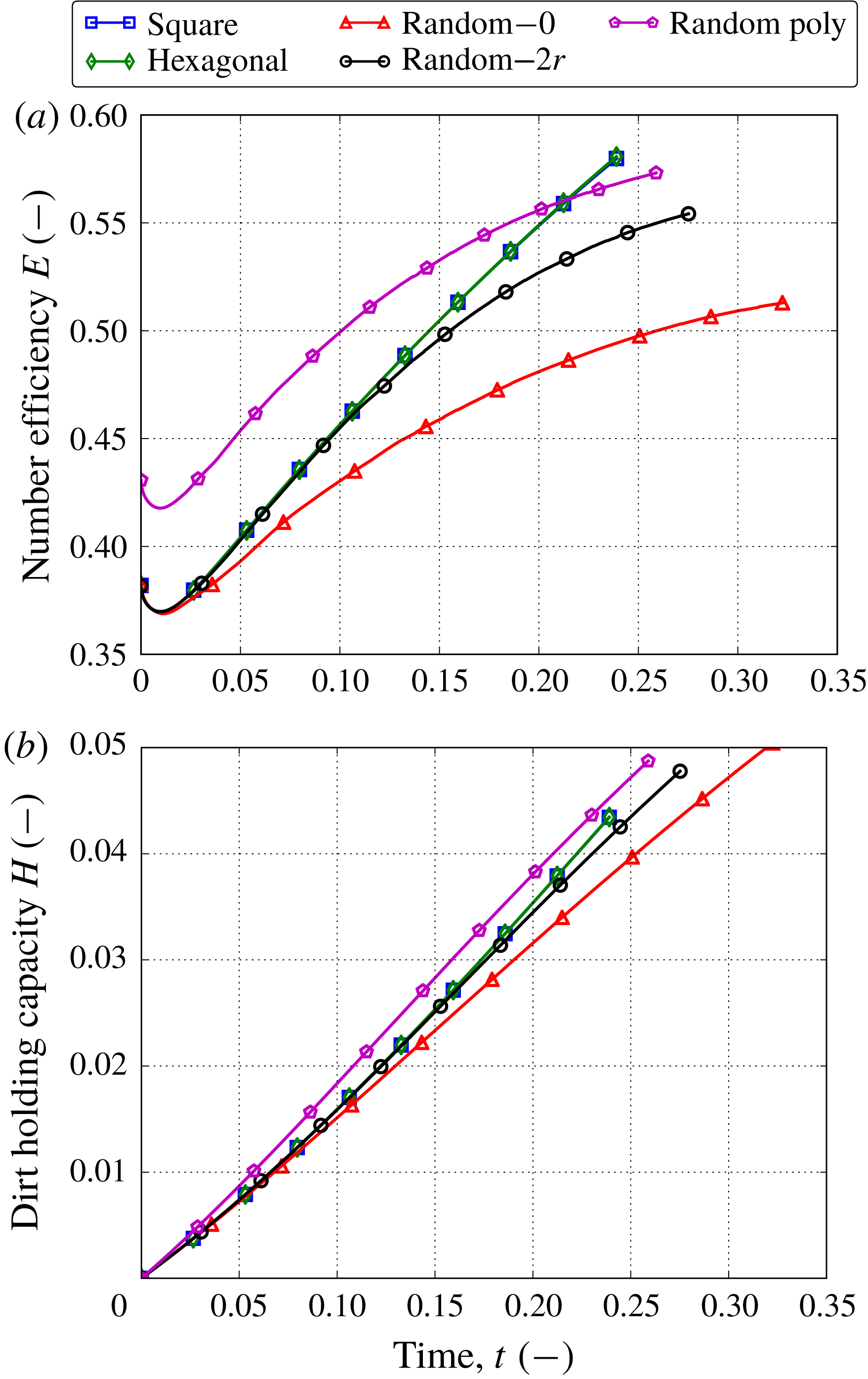
Figure 13. Multiscale simulation results for diffusion regime. We show the number efficiency
 $E$
(a) and the dirt-holding capacity
$E$
(a) and the dirt-holding capacity
 $H$
(b) as functions of time
$H$
(b) as functions of time
 $t$
.
$t$
.
This regime is influenced more by the microstructure type than by the filtration regimes with the constant flow rate, but is less sensitive to the microstructure than regimes with the constant pressure drop. The best choice of the microstructure depends on the priorities of the filtration: the efficiency or the lifetime. The highest efficiency is exhibited by the random microstructure with polydisperse fibres; but if the lifetime is more important than the filtration efficiency, then the random microstructure with isolation distance
 $2r$
becomes appealing.
$2r$
becomes appealing.
The lifetime of a filter medium
 $T$
is determined by the time at which a minimum prescribed value of the porosity is reached at any location of the filter medium. For our filtration set-ups, this location is always at the inflow boundary,
$T$
is determined by the time at which a minimum prescribed value of the porosity is reached at any location of the filter medium. For our filtration set-ups, this location is always at the inflow boundary,
 $x=0$
, where the maximum concentration and respectively the maximum of the contaminant adsorption are. The diffusion filtration regime has constant concentration at the inflow (see (4.11)). The advection and
$x=0$
, where the maximum concentration and respectively the maximum of the contaminant adsorption are. The diffusion filtration regime has constant concentration at the inflow (see (4.11)). The advection and
 $\overline{U}_{in}=\text{const.}$
regime also has constant inflow concentration due to the negligible diffusion term, which transforms the constant contaminant influx condition (4.6a
) into a Dirichlet boundary condition for the concentration. For both of these filtration regimes, the porosity at
$\overline{U}_{in}=\text{const.}$
regime also has constant inflow concentration due to the negligible diffusion term, which transforms the constant contaminant influx condition (4.6a
) into a Dirichlet boundary condition for the concentration. For both of these filtration regimes, the porosity at
 $x=0$
evolves in time according to (2.20) in exactly the same way due to the constant concentration. Therefore, we also observe that the dimensionless lifetime values for these regimes coincide exactly in figure 10. However, we note that the dimensional lifetime will be different for these filtration regimes because the time scaling
$x=0$
evolves in time according to (2.20) in exactly the same way due to the constant concentration. Therefore, we also observe that the dimensionless lifetime values for these regimes coincide exactly in figure 10. However, we note that the dimensional lifetime will be different for these filtration regimes because the time scaling
 ${\mathcal{T}}$
for diffusion- and advection-dominated processes are different.
${\mathcal{T}}$
for diffusion- and advection-dominated processes are different.
6 Transport mechanisms of filtration
Our simulation results show that, when including diffusion as a transport mechanism while maintaining a constant advection, the initial efficiency decreases – see, for example, figure 11. In this section we consider a simplified version of our homogenized model to understand the relative contributions of diffusion and advection. We note that we assume that the adsorption rate is fixed, although in reality this may change with changes in the contaminant diffusivity.
We consider the initial filtration behaviour before any changes in the porosity affect the microstructure and the filter efficiency. Then, we are concerned with the steady-state version of (2.15), that is,
 $C(x,t=0)\equiv C(x)$
. We assume that the initial microstructure has no macroscopic variations throughout the medium depth, that is,
$C(x,t=0)\equiv C(x)$
. We assume that the initial microstructure has no macroscopic variations throughout the medium depth, that is,
 $\unicode[STIX]{x1D719}$
,
$\unicode[STIX]{x1D719}$
,
 ${\mathcal{D}}$
and
${\mathcal{D}}$
and
 ${\mathcal{A}}$
are constant. The fluid velocity
${\mathcal{A}}$
are constant. The fluid velocity
 $\overline{U}$
is also constant because we do not consider changes in the microstructure. We focus on the case when the contaminant influx is prescribed (see (4.6)). Then, the filtration model (2.15) in 1D reads
$\overline{U}$
is also constant because we do not consider changes in the microstructure. We focus on the case when the contaminant influx is prescribed (see (4.6)). Then, the filtration model (2.15) in 1D reads
 $$\begin{eqnarray}\displaystyle & \displaystyle -a\frac{\text{d}^{2}C}{\text{d}x^{2}}+b\frac{\text{d}C}{\text{d}x}+C=0,\quad x\in (0,1), & \displaystyle\end{eqnarray}$$
 $$\begin{eqnarray}\displaystyle & \displaystyle -a\frac{\text{d}C}{\text{d}x}+bC=c,\quad x=0, & \displaystyle\end{eqnarray}$$
 $$\begin{eqnarray}\displaystyle & \displaystyle \frac{\text{d}C}{\text{d}x}=0,\quad x=1, & \displaystyle\end{eqnarray}$$
 $a$
,
$a$
,
 $b$
and
$b$
and
 $c$
are defined as
$c$
are defined as  $$\begin{eqnarray}a=\frac{\unicode[STIX]{x1D6FE}\unicode[STIX]{x1D719}{\mathcal{D}}}{{\mathcal{A}}},\quad b=\frac{\unicode[STIX]{x1D701}\overline{U}}{{\mathcal{A}}},\quad c=\frac{J_{in}}{{\mathcal{A}}}.\end{eqnarray}$$
The solution of (6.1) is given by
 $$\begin{eqnarray}C(x)=K_{1}\exp (\unicode[STIX]{x1D706}_{1}x)+K_{2}\exp (\unicode[STIX]{x1D706}_{2}x),\end{eqnarray}$$
where
 $$\begin{eqnarray}\displaystyle & \displaystyle \unicode[STIX]{x1D706}_{1,2}=\frac{b\pm \sqrt{b^{2}+4a}}{2a}, & \displaystyle\end{eqnarray}$$
 $$\begin{eqnarray}\displaystyle & \displaystyle K_{i}=c\left(b-a\unicode[STIX]{x1D706}_{i}-\frac{\unicode[STIX]{x1D706}_{i}\exp (\unicode[STIX]{x1D706}_{i})}{\unicode[STIX]{x1D706}_{j}\exp (\unicode[STIX]{x1D706}_{j})}(b-a\unicode[STIX]{x1D706}_{j})\right)^{-1},\quad i,j=1,2,~i\neq j. & \displaystyle\end{eqnarray}$$
The initial number efficiency is, from (4.1),
 $$\begin{eqnarray}E(t=0)\equiv E_{0}=1-\frac{b}{c}C(1).\end{eqnarray}$$
We find that the time
 $t^{\ast }$
that a single contaminant particle takes to transit the filter is
$t^{\ast }$
that a single contaminant particle takes to transit the filter is
 $$\begin{eqnarray}t^{\ast }=\int _{0}^{1}\frac{C(x)}{J_{C}(x)}\,\text{d}x.\end{eqnarray}$$
Since we are interested in the contributions of the diffusion and advection transport mechanisms, which are represented by the parameters
 $a$
and
$a$
and
 $b$
, respectively, let us assume that
$b$
, respectively, let us assume that
 $c=1$
. Figure 14 shows the initial efficiency
$c=1$
. Figure 14 shows the initial efficiency
 $E_{0}$
as a function of
$E_{0}$
as a function of
 $a$
and
$a$
and
 $b$
. This corroborates our simulation results that, as diffusion gets smaller, the efficiency increases. Similarly, the efficiency increases when we reduce the advection. Overall, the behaviour of the number efficiency is monotonic with respect to the advection and diffusion terms.
$b$
. This corroborates our simulation results that, as diffusion gets smaller, the efficiency increases. Similarly, the efficiency increases when we reduce the advection. Overall, the behaviour of the number efficiency is monotonic with respect to the advection and diffusion terms.
Figure 15 shows the transit time
 $t^{\ast }$
as a function of the parameters
$t^{\ast }$
as a function of the parameters
 $a$
and
$a$
and
 $b$
. A larger diffusion
$b$
. A larger diffusion
 $a$
means that, for the same concentration gradient, the transport of the contaminant will be faster. Therefore, as
$a$
means that, for the same concentration gradient, the transport of the contaminant will be faster. Therefore, as
 $a$
increases, the transit time
$a$
increases, the transit time
 $t^{\ast }$
reduces, along with the chance for this particle to adhere to the fibre surface, which yields lower efficiency. The same holds for the increased advection
$t^{\ast }$
reduces, along with the chance for this particle to adhere to the fibre surface, which yields lower efficiency. The same holds for the increased advection
 $b$
, and we observe a monotonic decrease of the transit time as
$b$
, and we observe a monotonic decrease of the transit time as
 $a$
and
$a$
and
 $b$
increase.
$b$
increase.
This offers a route towards improving the filtration efficiency, and quantifying the improvements gained, by adjusting the parameters of the filtration set-up. However, we note that these conclusions are made based on the assumption of a constant adsorption coefficient, whereas in real filtration processes this adsorption might change with filtration parameters, space and time, as discussed earlier.
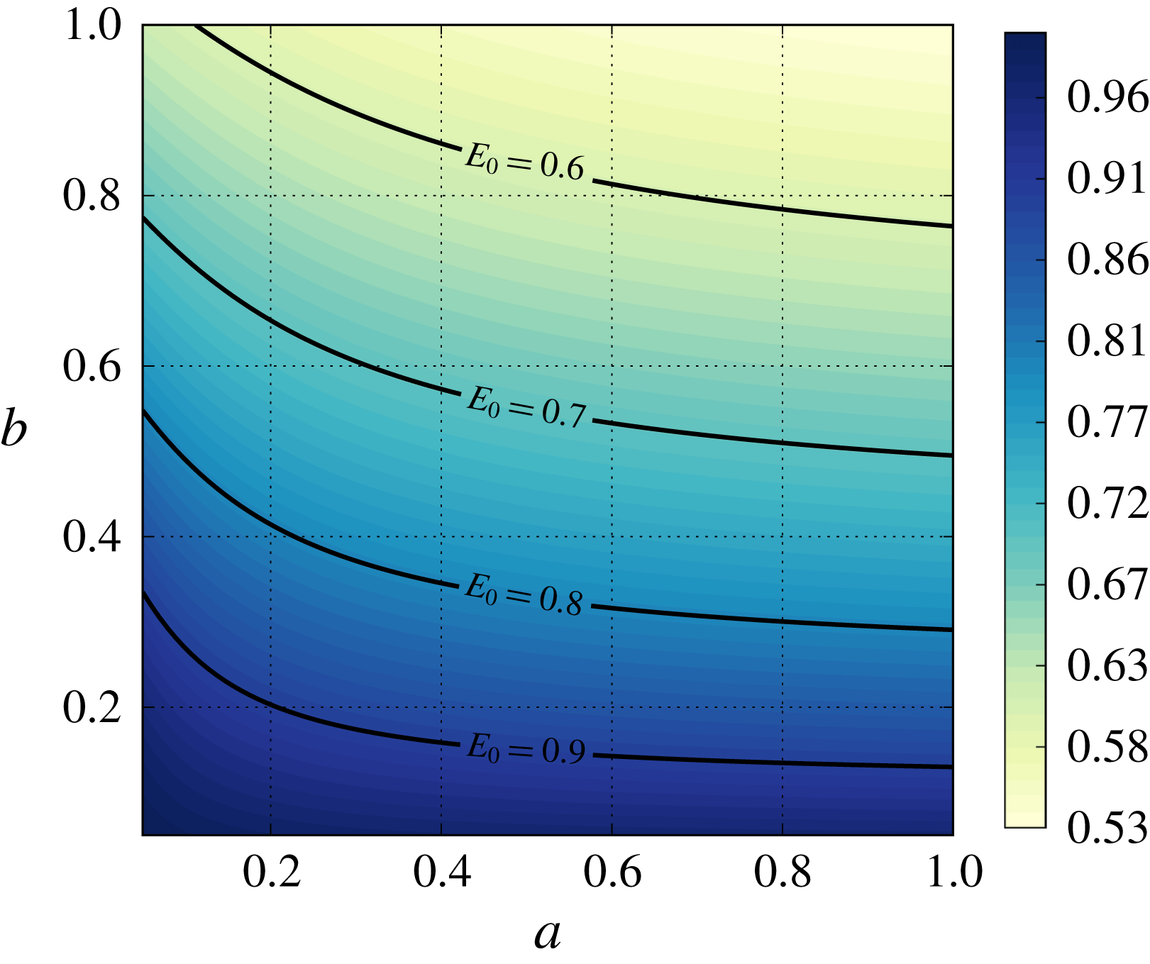
Figure 14. The initial efficiency
 $E_{0}$
as a function of the parameters
$E_{0}$
as a function of the parameters
 $a$
and
$a$
and
 $b$
.
$b$
.
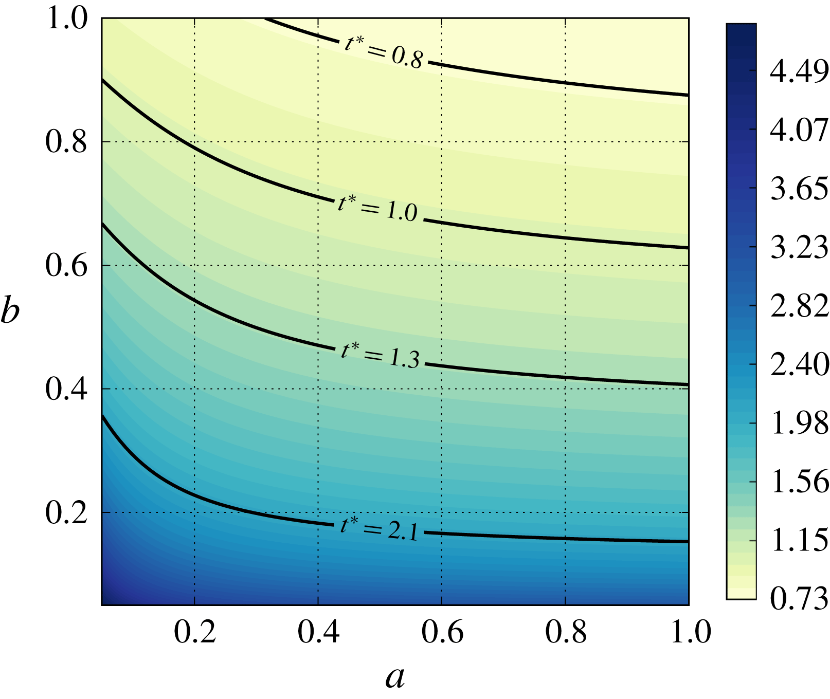
Figure 15. The time
 $t^{\ast }$
taken by a contaminant particle to transit the filter as a function of the parameters
$t^{\ast }$
taken by a contaminant particle to transit the filter as a function of the parameters
 $a$
and
$a$
and
 $b$
.
$b$
.
7 Conclusions
In this study, we obtained a multiscale model using the method of multiple scales to simulate contaminant filtration in fibrous filter media with unidirectional fibres. Our main contribution was to study how sensitive filter performance is to the microstructure under different filtration regimes. First, we extended the homogenization model of Dalwadi et al. (Reference Dalwadi, Griffiths and Bruna2015, Reference Dalwadi, Bruna and Griffiths2016) to account for random microstructures and fibres with different sizes in the same unit cell. Second, we proposed an agglomeration algorithm to model the process whereby fibres that are located close to one another agglomerate as contaminant deposits on their surface.
In filtration processes, it is important to be able to account for non-uniform filter porosities: these appear in porosity-graded filters, but also in standard uniform filters that become porosity-graded as contaminant is deposited in a non-uniform way in its depth. In our model, we accounted for non-uniform porosity by allowing the microscopic cell geometry to vary with the macroscopic variable. The advantage of this approach is that we were able to parametrize the non-uniform microstructure via the porosity
 $\unicode[STIX]{x1D719}$
and compute the effective parameters in the homogenized model (the permeability
$\unicode[STIX]{x1D719}$
and compute the effective parameters in the homogenized model (the permeability
 ${\mathcal{K}}$
, the effective diffusivity
${\mathcal{K}}$
, the effective diffusivity
 ${\mathcal{D}}$
and the effective surface area
${\mathcal{D}}$
and the effective surface area
 ${\mathcal{A}}$
) as functions of
${\mathcal{A}}$
) as functions of
 $\unicode[STIX]{x1D719}$
as a pre-processing step. In other words, there is a one-way coupling between the microscopic model (the cell problems) and the macroscopic homogenized model describing the evolution of the contaminant concentration across the filter depth. The disadvantage is that it requires the microstructure to be locally periodic, so large variations in porosity are not allowed. This is in contrast with the more general work by Ray et al. (Reference Ray, Elbinger and Knabner2015), which requires the cell problems to be solved at every macroscopic location.
$\unicode[STIX]{x1D719}$
as a pre-processing step. In other words, there is a one-way coupling between the microscopic model (the cell problems) and the macroscopic homogenized model describing the evolution of the contaminant concentration across the filter depth. The disadvantage is that it requires the microstructure to be locally periodic, so large variations in porosity are not allowed. This is in contrast with the more general work by Ray et al. (Reference Ray, Elbinger and Knabner2015), which requires the cell problems to be solved at every macroscopic location.
Thanks to the one-way coupling, our model provides an efficient simulation tool that can handle not only regular microstructures (for example, square and hexagonal) but also random microstructures (random arrangements of fibres in a unit cell that are extended periodically). We investigated five types of microstructures: square, hexagonal, two random with different isolation distances between fibres, and random with polydisperse fibre radii. These microstructures provide us with different degrees of randomness. The hexagonal microstructure is the limiting case of a random microstructure with large isolation distance (as the hexagonal lattice maximizes the separation distance between fibres), while the purely random one is with zero isolation distance. The microscale simulations showed that the permeability
 ${\mathcal{K}}$
and the effective surface area
${\mathcal{K}}$
and the effective surface area
 ${\mathcal{A}}$
are very sensitive to the microstructure of the fibrous media, but the effective diffusivity
${\mathcal{A}}$
are very sensitive to the microstructure of the fibrous media, but the effective diffusivity
 ${\mathcal{D}}$
is less so.
${\mathcal{D}}$
is less so.
We considered five different filtration regimes and investigated how sensitive the final filtration results are to the microstructure type. We summarize our findings below.
(i) Advection–diffusion and advection regimes with
$\overline{U}_{in}=\text{const.}$
: the best choice for the microstructure is random with polydisperse fibre radii. This set-up provides the best number efficiency and dirt-holding capacity among the microstructures considered, and its pressure does not rise very much during the whole lifetime of the filter medium. However, while an optimum microstructure exists, the performance in this regime is only weakly affected by the microstructure choice, and all other microstructures perform almost as well (see table 3).(ii) Advection–diffusion and advection regimes with
$\unicode[STIX]{x0394}P=\text{const.}$
: the random microstructure with isolation distance
$2r$
balances all the performance criteria. It offers good efficiency while providing the second largest throughput and lifetime. Filtration is a lot more sensitive to the microstructure in these regimes.(iii) Diffusion regime: again, the random microstructure with polydisperse fibre radii exhibits the best efficiency results, while the random microstructure with no isolation distance has the longest lifetime. This regime has a moderate sensitivity to the microstructure in comparison with the other filtration regimes.


To understand the interplay between the transport mechanisms in the filtration, we investigated how the diffusion and advection terms affect the efficiency results. We found that the initial number efficiency decreases monotonically as we increase the strength of their dimensionless groups. This behaviour is explained by the fact that larger diffusion or advection leads to a faster transport of contaminant across the filter medium and consequently less time for them to adhere to the fibre surface.
Our multiscale model can be used to make predictions about filter performance and to optimize its porosity or microstructure depending on the requirements of the application. This could range from air-conditioning systems, to the pharmaceutical and biotechnology industries. Predicting experimental data with a mathematical tool always introduces additional challenges: defining realistic parameters that cannot be measured (for example, the adsorption coefficient) and accounting for additional features of real-life processes (for example, polydisperse contaminants and parameter uncertainties). Moreover, we will also extend this model to account for additional effects that can influence the filtration performance, such as electrostatic effects in air filtration. This will require deriving a new mathematical model accounting for more physical complexity while having the similar objective of developing a simple and efficient tool.
In the wider context, the mathematical framework that we have laid out applies to a range of other problems in which obstacle growth and coalescence are important. For example, in the application of tissue engineering and cell growth, the model may be used to understand the effect that irregularities in the scaffold have on the rate of tissue growth. The problem may also be studied in reverse, whereby material is being removed from rather than deposited onto obstacles. Such a scenario may occur in various geological applications with dissolution of porous media or in cases where the goal is to remove a particular substance, such as in the decontamination of a chemical from porous media (Dalwadi et al. Reference Dalwadi, O’Kiely, Thomson, Khaleque and Hall2017). The model could also be generalized to account for transfer of material from obstacle to obstacle, mimicking scenarios such as Ostwald ripening (Voorhees Reference Voorhees1985).
Acknowledgements
This publication was made possible by an EPSRC Impact Acceleration Account, grant EP/K503769/1, and research funding from Dyson Ltd. The authors would like to thank the Dyson staff, in particular G. Morris, B. Hovell, T. Grimble and S. Koch, for inspiring this research project and for fruitful discussions on the problem understanding and research directions. I.M.G. is grateful to the Royal Society for funding through a University Research Fellowship. M.B. is grateful to St John’s College, Oxford, for funding through a Junior Research Fellowship.
Appendix. Convergence test for closely located fibres
As the distance between two fibres tends to zero, the diagonal elements of the Jacobian matrix of
 $\unicode[STIX]{x1D71E}$
, which is a solution to the cell problem (2.17), tend to infinity in a domain whose measure tends to zero. To make sure that this numerical effect does not cause problems while computing the effective diffusivity
$\unicode[STIX]{x1D71E}$
, which is a solution to the cell problem (2.17), tend to infinity in a domain whose measure tends to zero. To make sure that this numerical effect does not cause problems while computing the effective diffusivity
 $\boldsymbol{{\mathcal{D}}}$
for the random microstructures, we perform a convergence test. If the coordinate origin is located at the centre of the unit cell, we consider two fibres with the centres located at
$\boldsymbol{{\mathcal{D}}}$
for the random microstructures, we perform a convergence test. If the coordinate origin is located at the centre of the unit cell, we consider two fibres with the centres located at
 $(-r-\unicode[STIX]{x1D716}/2,0)$
and
$(-r-\unicode[STIX]{x1D716}/2,0)$
and
 $(r+\unicode[STIX]{x1D716}/2,0)$
, assuming that
$(r+\unicode[STIX]{x1D716}/2,0)$
, assuming that
 $\unicode[STIX]{x1D6FF}l/r=9.47$
and
$\unicode[STIX]{x1D6FF}l/r=9.47$
and
 $\unicode[STIX]{x1D719}=0.93$
. To obtain a reference solution, we use a unit cell with the limiting case, that is, when the two fibres are just in contact and form a connected ‘infinity-shaped’ volume. Then, we compute a relative error of the effective diffusivity as a function of
$\unicode[STIX]{x1D719}=0.93$
. To obtain a reference solution, we use a unit cell with the limiting case, that is, when the two fibres are just in contact and form a connected ‘infinity-shaped’ volume. Then, we compute a relative error of the effective diffusivity as a function of
 $\unicode[STIX]{x1D700}$
(see figure 16).
$\unicode[STIX]{x1D700}$
(see figure 16).
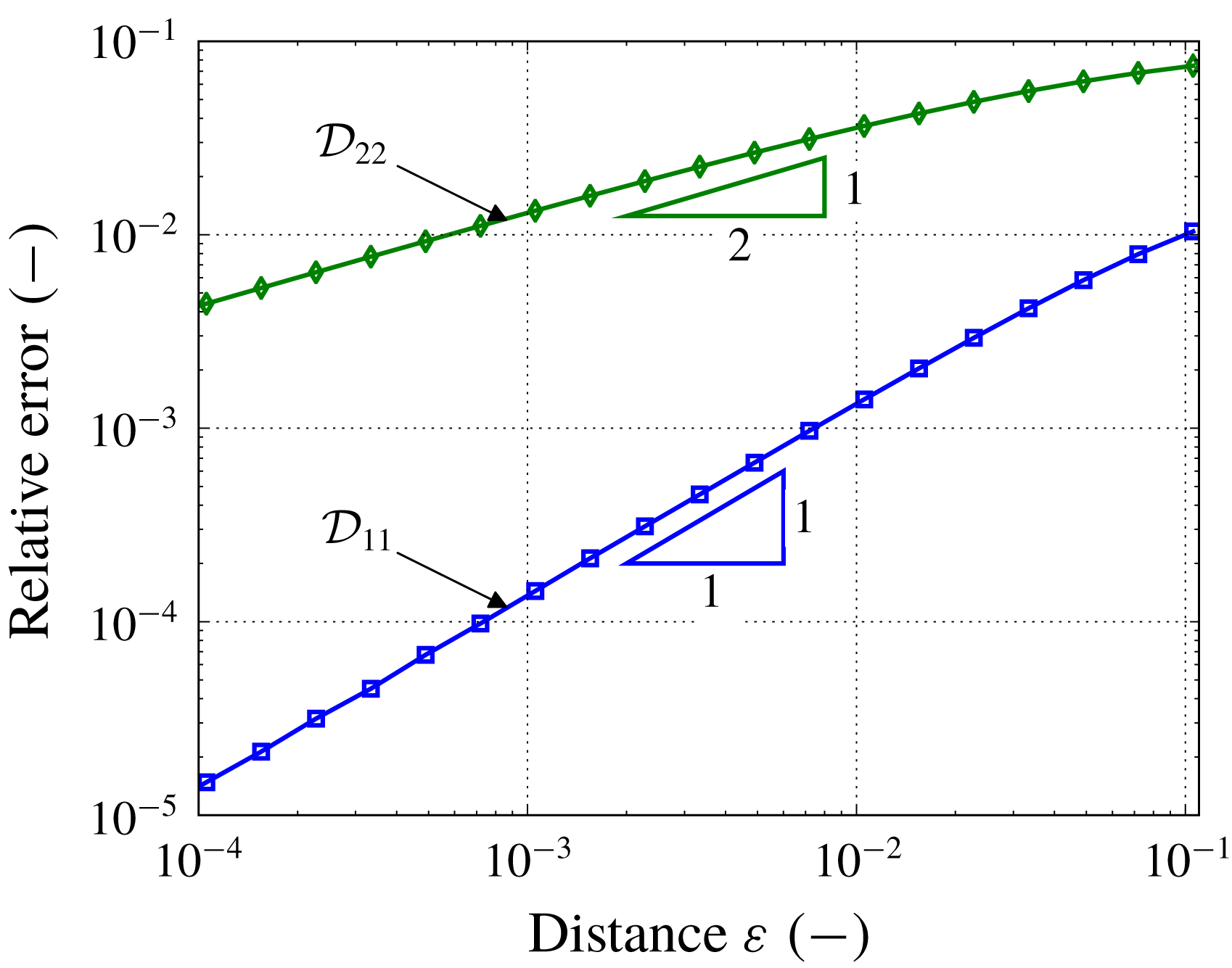
Figure 16. Relative error between two close fibres and the limiting case of two touching fibres as a function of the distance between the two close fibres.
The estimation of the relative error requires a refinement around the fibres, which poses a restriction on the smallest size of the critical distance that we can consider. We are able to estimate the error for critical distances
 $\unicode[STIX]{x1D700}$
up to
$\unicode[STIX]{x1D700}$
up to
 $10^{-4}$
(see figure 16), which show a monotonic convergence of the effective parameters for the two closely located fibres to the limiting case with two joined fibres. The relative error for the diagonal elements of the effective diffusivity
$10^{-4}$
(see figure 16), which show a monotonic convergence of the effective parameters for the two closely located fibres to the limiting case with two joined fibres. The relative error for the diagonal elements of the effective diffusivity
 $\boldsymbol{{\mathcal{D}}}$
is less than
$\boldsymbol{{\mathcal{D}}}$
is less than
 $10^{-2}$
for the critical distance
$10^{-2}$
for the critical distance
 $\unicode[STIX]{x1D700}=10^{-4}$
. This distance is usually less than the average size of a contaminant particle and it is likely to be blocked by a single particle, which yields the formation of an agglomerate in a real filtration process. Hence, forming the agglomerates for distances around
$\unicode[STIX]{x1D700}=10^{-4}$
. This distance is usually less than the average size of a contaminant particle and it is likely to be blocked by a single particle, which yields the formation of an agglomerate in a real filtration process. Hence, forming the agglomerates for distances around
 $10^{-4}$
in the modelling process not only produces small errors, but is also justified from a physical standpoint.
$10^{-4}$
in the modelling process not only produces small errors, but is also justified from a physical standpoint.