


1 Introduction
The presence of floating vegetation in fresh-water systems (e.g. lakes) can affect water chemistry (Zhang & Nepf Reference Zhang and Nepf2011) and impact biomass and fish habitat (Adams et al. Reference Adams, Boar, Hubble, Gikundgu, Harper, Hickley and Tarras-Wahlberg2002; Padial, Thomas & Agostinho Reference Padial, Thomas and Agostinho2009). Generally, floating vegetation develops in shallow, quiescent regions, where the background flow can be neglected (Azza et al. Reference Azza, Denny, van de Koppel and Kansiime2006). Under such conditions, an exchange flow may develop between the zones with and without floating vegetation, and this convective exchange flow will dominate the mass exchange between the vegetated and the open-water regions. This exchange flow is driven by temperature differences associated with different solar heating between the shaded regions containing floating vegetation and the adjacent open-water regions (Chimney, Wenkert & Pietro Reference Chimney, Wenkert and Pietro2006). Differences in solar heating have also been observed between surface-water regions with different concentrations of phytoplankton that alter the penetration of solar radiation through the water column (Edwards, Wright & Platt Reference Edwards, Wright and Platt2004), and between regions of rooted vegetation adjacent to open water (Lovstedt & Bengtsson Reference Lovstedt and Bengtsson2008).
Previous studies have reported differences of
 $1{-}2\,^{\circ }\text{C}$
between regions containing water hyacinths and the surrounding open water (Ultsch Reference Ultsch1973), and between marsh regions and an adjacent open pond (Lightbody, Avener & Nepf Reference Lightbody, Avener and Nepf2008). The temperature difference follows the diurnal cycle of heating and cooling, with zero temperature difference from midnight to approximately 6 am, followed by a gradual increase to a peak in mid-afternoon and returning to zero again at midnight (e.g. see figure 14 in Lightbody et al.
Reference Lightbody, Avener and Nepf2008). Because the forcing for the exchange current is absent during the night and restarts each morning, it is reasonable to use a lock exchange as a first-order model for the flow initiated each day. Finally, if the depth of the two regions is relatively small, the vertical temperature gradient in each region is negligible, such that the temperature in the open water and vegetated regions may each be considered vertically uniform, approximating the initial conditions of a lock exchange. In fact, even when a mild vertical stratification is present, due to differential light absorption over the depth, the vertical stratification had minimal effect on the development of the free-surface exchange current (Coates & Paterson Reference Coates and Paterson1993; Zhang & Nepf Reference Zhang and Nepf2011). The lock-exchange model neglects the variation of the temperature difference between vegetation and open water throughout the day. Therefore, the assumption of a constant density difference is a simplification. The simplification of a constant temperature difference, e.g. set at the average difference over the day, has been used in previous studies of exchange flow in lakes and shown to yield velocity scales of the correct order of magnitude (e.g. Andradottir & Nepf Reference Andradottir and Nepf2001).
$1{-}2\,^{\circ }\text{C}$
between regions containing water hyacinths and the surrounding open water (Ultsch Reference Ultsch1973), and between marsh regions and an adjacent open pond (Lightbody, Avener & Nepf Reference Lightbody, Avener and Nepf2008). The temperature difference follows the diurnal cycle of heating and cooling, with zero temperature difference from midnight to approximately 6 am, followed by a gradual increase to a peak in mid-afternoon and returning to zero again at midnight (e.g. see figure 14 in Lightbody et al.
Reference Lightbody, Avener and Nepf2008). Because the forcing for the exchange current is absent during the night and restarts each morning, it is reasonable to use a lock exchange as a first-order model for the flow initiated each day. Finally, if the depth of the two regions is relatively small, the vertical temperature gradient in each region is negligible, such that the temperature in the open water and vegetated regions may each be considered vertically uniform, approximating the initial conditions of a lock exchange. In fact, even when a mild vertical stratification is present, due to differential light absorption over the depth, the vertical stratification had minimal effect on the development of the free-surface exchange current (Coates & Paterson Reference Coates and Paterson1993; Zhang & Nepf Reference Zhang and Nepf2011). The lock-exchange model neglects the variation of the temperature difference between vegetation and open water throughout the day. Therefore, the assumption of a constant density difference is a simplification. The simplification of a constant temperature difference, e.g. set at the average difference over the day, has been used in previous studies of exchange flow in lakes and shown to yield velocity scales of the correct order of magnitude (e.g. Andradottir & Nepf Reference Andradottir and Nepf2001).
The free-surface current containing warmer water originating in the open region displaces colder water within the vegetated region containing the plant stems, also referred as the root or porous layer. The residence time of water within the root layer, where biochemical reactions occur, is an important variable in determining how the floating vegetation impacts the water quality of the surrounding water. The root zone residence time depends on the speed of the free surface current. The speed of the surface current is a function of the difference in temperature between the two regions and the geometric characteristics of the root layer. The latter determines the drag force acting on the surface current within the root layer. For most practical applications (e.g. see discussion in Lovstedt & Bengtsson Reference Lovstedt and Bengtsson2008; Zhang & Nepf Reference Zhang and Nepf2008, Reference Zhang and Nepf2011), the drag added by the plant stems is sufficiently large for the flow within the root layer to be controlled by an equilibrium between buoyancy and drag forces (drag-dominated regime).
To understand the fundamental physics of this type of exchange flow, we will consider a lock-exchange flow in a long shallow channel with a length (
 $2L$
) to height (
$2L$
) to height (
 $H$
) ratio of
$H$
) ratio of
 $2L/H\gg 1$
, with the lock located at mid-length (figure 1), which produces a high volume release. The canonical case of a lock-exchange flow developing in a channel filled with identical cylinders and containing water of different temperatures was studied experimentally by Tanino, Nepf & Kulis (Reference Tanino, Nepf and Kulis2005) and numerically by Ozan, Constantinescu & Hogg (Reference Ozan, Constantinescu and Hogg2015). This limiting case will be referred as the fully vegetated case (figure 1
a). In the applications discussed in the present study, half of the channel
$2L/H\gg 1$
, with the lock located at mid-length (figure 1), which produces a high volume release. The canonical case of a lock-exchange flow developing in a channel filled with identical cylinders and containing water of different temperatures was studied experimentally by Tanino, Nepf & Kulis (Reference Tanino, Nepf and Kulis2005) and numerically by Ozan, Constantinescu & Hogg (Reference Ozan, Constantinescu and Hogg2015). This limiting case will be referred as the fully vegetated case (figure 1
a). In the applications discussed in the present study, half of the channel
 $(-L<x<0)$
contains a surface porous layer of constant depth,
$(-L<x<0)$
contains a surface porous layer of constant depth,
 $h_{1}<H$
(figure 1
b). In practical applications, this layer contains the roots of floating vegetation. The vegetated region
$h_{1}<H$
(figure 1
b). In practical applications, this layer contains the roots of floating vegetation. The vegetated region
 $(-L<x<0)$
is initially filled with heavier, lower-temperature fluid, while the open-water region
$(-L<x<0)$
is initially filled with heavier, lower-temperature fluid, while the open-water region
 $(0<x<L)$
is filled with lighter, higher-temperature fluid. This is the configuration studied experimentally by Zhang & Nepf (Reference Zhang and Nepf2011).
$(0<x<L)$
is filled with lighter, higher-temperature fluid. This is the configuration studied experimentally by Zhang & Nepf (Reference Zhang and Nepf2011).

Figure 1. Sketch showing the evolution of a lock-exchange flow in a fully vegetated channel (a) and in a partially vegetated channel containing a vegetated (porous) layer at the free surface (b). The heavier fluid is shown in grey. The lighter fluid is shown in white. The front velocity of the free-surface current is
 $U_{f}$
and its distance to the lock gate is
$U_{f}$
and its distance to the lock gate is
 $|x_{f}|$
. The evolution of the lock-exchange flow is close to anti-symmetric in the fully vegetated case. The horizontal (red) arrows in (b) denote the velocities in the porous and intrusion layers. The (blue) arrows pointing down and the (green) arrows pointing up in (b) show regions where mass exchange between the porous and intrusion layers is strong. Arrows pointing downwards show flow being advected out of the porous layer while arrows pointing upwards show flow being advected into the porous layer.
$|x_{f}|$
. The evolution of the lock-exchange flow is close to anti-symmetric in the fully vegetated case. The horizontal (red) arrows in (b) denote the velocities in the porous and intrusion layers. The (blue) arrows pointing down and the (green) arrows pointing up in (b) show regions where mass exchange between the porous and intrusion layers is strong. Arrows pointing downwards show flow being advected out of the porous layer while arrows pointing upwards show flow being advected into the porous layer.
In the present simulations, the porous layer is characterized by the solid volume fraction,
 $\unicode[STIX]{x1D719}$
, the height of the porous layer,
$\unicode[STIX]{x1D719}$
, the height of the porous layer,
 $h_{1}$
, the edge length of the square cylinders,
$h_{1}$
, the edge length of the square cylinders,
 $D$
, the non-dimensional frontal area of the cylinders per unit volume,
$D$
, the non-dimensional frontal area of the cylinders per unit volume,
 $ah_{1}$
, the orientation of the cylinders and their arrangement. The variable
$ah_{1}$
, the orientation of the cylinders and their arrangement. The variable
 $\unicode[STIX]{x1D719}$
is defined as the ratio of volume occupied by the square cylinders to the total volume of the porous layer. For square cylinders,
$\unicode[STIX]{x1D719}$
is defined as the ratio of volume occupied by the square cylinders to the total volume of the porous layer. For square cylinders,
 $ah_{1}=\unicode[STIX]{x1D719}h_{1}/D$
. As the flow around the individual cylinders is resolved by the numerical simulations, there is no need to provide a cylinder drag coefficient or to model the effects of the wake-to-cylinder interactions on flow and turbulence generation, as usually done in models that do not resolve the flow around individual cylinders (e.g. see Jamali, Zhang & Nepf Reference Jamali, Zhang and Nepf2008; King, Tinoco & Cowen Reference King, Tinoco and Cowen2012).
$ah_{1}=\unicode[STIX]{x1D719}h_{1}/D$
. As the flow around the individual cylinders is resolved by the numerical simulations, there is no need to provide a cylinder drag coefficient or to model the effects of the wake-to-cylinder interactions on flow and turbulence generation, as usually done in models that do not resolve the flow around individual cylinders (e.g. see Jamali, Zhang & Nepf Reference Jamali, Zhang and Nepf2008; King, Tinoco & Cowen Reference King, Tinoco and Cowen2012).
High-volume-of-release currents propagating in channels with no obstacles and no large-scale bottom roughness rapidly reach a slumping phase in which the front velocity,
 $U_{f}$
, is constant (Rottman & Simpson Reference Rottman and Simpson1983). If the channel is filled with identical cylinders that are close to uniformly distributed (figure 1
a), the current initially experiences a slumping phase, but, if
$U_{f}$
, is constant (Rottman & Simpson Reference Rottman and Simpson1983). If the channel is filled with identical cylinders that are close to uniformly distributed (figure 1
a), the current initially experiences a slumping phase, but, if
 $\unicode[STIX]{x1D719}$
is large enough, eventually
$\unicode[STIX]{x1D719}$
is large enough, eventually
 $U_{f}$
decays with time, even if the front is far from the end walls (Hatcher, Hogg & Woods Reference Hatcher, Hogg and Woods2000; Tanino et al.
Reference Tanino, Nepf and Kulis2005). This corresponds to the transition to the drag-dominated regime, in which inertial forces are relatively small and the flow is determined by a balance between buoyancy and the drag forces induced by the cylinders. High Reynolds number lock-exchange flows are defined as currents for which the cylinder Reynolds number,
$U_{f}$
decays with time, even if the front is far from the end walls (Hatcher, Hogg & Woods Reference Hatcher, Hogg and Woods2000; Tanino et al.
Reference Tanino, Nepf and Kulis2005). This corresponds to the transition to the drag-dominated regime, in which inertial forces are relatively small and the flow is determined by a balance between buoyancy and the drag forces induced by the cylinders. High Reynolds number lock-exchange flows are defined as currents for which the cylinder Reynolds number,
 $Re_{D}=DU/\unicode[STIX]{x1D708}$
(
$Re_{D}=DU/\unicode[STIX]{x1D708}$
(
 $\unicode[STIX]{x1D708}$
is the molecular viscosity), defined with a velocity scale characterizing the mean approaching velocity for the cylinders within the array (e.g.
$\unicode[STIX]{x1D708}$
is the molecular viscosity), defined with a velocity scale characterizing the mean approaching velocity for the cylinders within the array (e.g.
 $U$
is sometime approximated by the front velocity,
$U$
is sometime approximated by the front velocity,
 $U_{f}$
), is much larger than unity for most of the cylinders situated inside the gravity current. Such currents generally transition first to a quadratic drag regime, in which the drag force is proportional to
$U_{f}$
), is much larger than unity for most of the cylinders situated inside the gravity current. Such currents generally transition first to a quadratic drag regime, in which the drag force is proportional to
 $U^{2}$
. In low Reynolds number cases
$U^{2}$
. In low Reynolds number cases
 $(Re_{D}<1)$
, the current transitions directly to a linear-drag regime in which the drag force is proportional to
$(Re_{D}<1)$
, the current transitions directly to a linear-drag regime in which the drag force is proportional to
 $U$
. Shallow-water theory predicts
$U$
. Shallow-water theory predicts
 $U_{f}\sim t^{-1/2}$
(
$U_{f}\sim t^{-1/2}$
(
 $x_{f}\sim t^{1/2}$
) for the linear-drag regime and
$x_{f}\sim t^{1/2}$
) for the linear-drag regime and
 $U_{f}\sim t^{-1/3}$
(
$U_{f}\sim t^{-1/3}$
(
 $x_{f}\sim t^{2/3}$
) for the quadratic-drag regime, where
$x_{f}\sim t^{2/3}$
) for the quadratic-drag regime, where
 $t$
is the time measured since the gate is released and
$t$
is the time measured since the gate is released and
 $x_{f}$
is the front position. Three-dimensional (3-D) large eddy simulation (LES) also predicts
$x_{f}$
is the front position. Three-dimensional (3-D) large eddy simulation (LES) also predicts
 $U_{f}\sim t^{-1/2}$
for the linear-drag regime, but predicts
$U_{f}\sim t^{-1/2}$
for the linear-drag regime, but predicts
 $U_{f}\sim t^{-1/4}$
during the quadratic-drag regime (Constantinescu Reference Constantinescu2014; Ozan et al.
Reference Ozan, Constantinescu and Hogg2015).
$U_{f}\sim t^{-1/4}$
during the quadratic-drag regime (Constantinescu Reference Constantinescu2014; Ozan et al.
Reference Ozan, Constantinescu and Hogg2015).
In the configuration studied in the present study (figure 1
b), the structure of the exchange flow is more complex compared to the previously discussed case of cylinders extending through the entire water depth. This is because the flow is no longer anti-symmetrical, i.e. only the surface current is directly impacted by the drag layer containing the cylinders and the bottom current is only indirectly impacted by the drag layer through the constraints of continuity. A second difference is that, except for the limiting full-depth case in which
 $h_{1}/H=1$
(Jamali et al.
Reference Jamali, Zhang and Nepf2008; Zhang & Nepf Reference Zhang and Nepf2008), or for cases with
$h_{1}/H=1$
(Jamali et al.
Reference Jamali, Zhang and Nepf2008; Zhang & Nepf Reference Zhang and Nepf2008), or for cases with
 $h_{1}/H$
close to 1, the surface current is broken into two layers. The fluid within the porous layer moves slowly through the obstructed region, while the layer beneath it, which we will refer to as the intrusion layer, moves faster (Zhang & Nepf Reference Zhang and Nepf2011). The depths of these two layers are denoted
$h_{1}/H$
close to 1, the surface current is broken into two layers. The fluid within the porous layer moves slowly through the obstructed region, while the layer beneath it, which we will refer to as the intrusion layer, moves faster (Zhang & Nepf Reference Zhang and Nepf2011). The depths of these two layers are denoted
 $h_{1}$
and
$h_{1}$
and
 $h_{2}(x,t)$
, respectively. The depth of the return current (third layer) is
$h_{2}(x,t)$
, respectively. The depth of the return current (third layer) is
 $h_{3}=H-h_{1}-h_{2}$
(figure 1
b).
$h_{3}=H-h_{1}-h_{2}$
(figure 1
b).
The case with
 $h_{1}/H<0.5$
was studied experimentally by Zhang & Nepf (Reference Zhang and Nepf2011). They also developed an analytical model that predicts the flow rates within the porous and intrusion layers during the drag-dominated regime. Their model assumes that the fluid velocity within the different layers is slowly varying with time. As with any shallow flow model, it also assumes the flow in each layer is predominantly horizontal. Because the channel length in their experiments was relatively short, the model was only calibrated based on the evolution of the surface current during the transition to the drag-dominated regime, when the decay of the front velocity with time is relatively small and the hypothesis of a steady flow is an acceptable assumption. In the present paper, the channel length is approximately twice as long as that in the experiments of Zhang & Nepf (Reference Zhang and Nepf2011). This allows us to study the structure of the current and its propagation long after the transition to the drag-dominated regime, when the front velocity is decaying rapidly with time, something that was not possible in the experiments of Zhang & Nepf (Reference Zhang and Nepf2011). Given that in most field applications the horizontal extent of the vegetated region is one to two orders of magnitude larger than the flow depth, the study of the flow structure during the later stages of the drag-dominated regime is of great practical importance and is the main focus of the present paper. Furthermore, the LES results from the present study demonstrate for the first time that there is significant vertical exchange between layers during the later stages of current evolution, such that analytical models based on shallow-water theory, like the ones proposed by Zhang & Nepf (Reference Zhang and Nepf2011), cannot be applied to accurately describe the overall evolution of the flow in the three layers. The vertical exchange controls the residence time within the porous layer. Finally, quantitative information regarding flow structure (e.g. temperature/density, velocity and vorticity fields, fluxes at the interface between the layers) and mixing is more difficult to extract from experimental observations (Hartel, Meiburg & Necker Reference Hartel, Meiburg and Necker2000; Ooi, Constantinescu & Weber Reference Ooi, Constantinescu and Weber2009). Because a well-resolved LES can provide these details, we are able to address the following important research questions about the fully drag-dominated stage of the current, which previous experimental studies have not addressed. Specifically:
$h_{1}/H<0.5$
was studied experimentally by Zhang & Nepf (Reference Zhang and Nepf2011). They also developed an analytical model that predicts the flow rates within the porous and intrusion layers during the drag-dominated regime. Their model assumes that the fluid velocity within the different layers is slowly varying with time. As with any shallow flow model, it also assumes the flow in each layer is predominantly horizontal. Because the channel length in their experiments was relatively short, the model was only calibrated based on the evolution of the surface current during the transition to the drag-dominated regime, when the decay of the front velocity with time is relatively small and the hypothesis of a steady flow is an acceptable assumption. In the present paper, the channel length is approximately twice as long as that in the experiments of Zhang & Nepf (Reference Zhang and Nepf2011). This allows us to study the structure of the current and its propagation long after the transition to the drag-dominated regime, when the front velocity is decaying rapidly with time, something that was not possible in the experiments of Zhang & Nepf (Reference Zhang and Nepf2011). Given that in most field applications the horizontal extent of the vegetated region is one to two orders of magnitude larger than the flow depth, the study of the flow structure during the later stages of the drag-dominated regime is of great practical importance and is the main focus of the present paper. Furthermore, the LES results from the present study demonstrate for the first time that there is significant vertical exchange between layers during the later stages of current evolution, such that analytical models based on shallow-water theory, like the ones proposed by Zhang & Nepf (Reference Zhang and Nepf2011), cannot be applied to accurately describe the overall evolution of the flow in the three layers. The vertical exchange controls the residence time within the porous layer. Finally, quantitative information regarding flow structure (e.g. temperature/density, velocity and vorticity fields, fluxes at the interface between the layers) and mixing is more difficult to extract from experimental observations (Hartel, Meiburg & Necker Reference Hartel, Meiburg and Necker2000; Ooi, Constantinescu & Weber Reference Ooi, Constantinescu and Weber2009). Because a well-resolved LES can provide these details, we are able to address the following important research questions about the fully drag-dominated stage of the current, which previous experimental studies have not addressed. Specifically:
-
(i) How does the vertical structure of the surface current depend on the main geometrical parameters (
 $\unicode[STIX]{x1D719},h_{1}/H$
)?
$\unicode[STIX]{x1D719},h_{1}/H$
)? -
(ii) What controls the residence time of fluid within the porous (root) layer?

The paper is structured as follows. The numerical model, the boundary conditions and the test cases are described in § 2. Section 3 discusses how the structure of the surface current changes as a function of the main geometrical parameters and the Reynolds number. Section 4 discusses how the characteristics of the porous layer and the Reynolds number affect mixing. Section 5 analyses the temporal evolutions of the front position for the free surface and bottom currents and of the discharge at the lock gate. Section 6 discusses the temporal growth of the volume of lighter fluid advancing through the porous layer, which is needed to estimate the flushing time of the heavier fluid within the porous layer by the surface current. Finally, § 7 provides some concluding comments, connecting the results to field studies and discussing the main similarities and differences with simpler cases in which the whole surface current advances in a porous layer.
2 Numerical model, test cases and model validation
The governing Navier–Stokes and density transport equations are solved in non-dimensional form with the channel height,
 $H$
, as the spatial scale and the buoyancy velocity,
$H$
, as the spatial scale and the buoyancy velocity,
 $u_{b}=\sqrt{g^{\prime }H}$
, as the velocity scale. The reduced gravity is
$u_{b}=\sqrt{g^{\prime }H}$
, as the velocity scale. The reduced gravity is
 $g^{\prime }=g(\unicode[STIX]{x1D70C}_{max}-\unicode[STIX]{x1D70C}_{min})/\unicode[STIX]{x1D70C}_{max}$
, where
$g^{\prime }=g(\unicode[STIX]{x1D70C}_{max}-\unicode[STIX]{x1D70C}_{min})/\unicode[STIX]{x1D70C}_{max}$
, where
 $g$
is the gravitational acceleration and
$g$
is the gravitational acceleration and
 $\unicode[STIX]{x1D70C}_{max}$
is the density of the colder fluid (with temperature
$\unicode[STIX]{x1D70C}_{max}$
is the density of the colder fluid (with temperature
 $T_{min}^{\prime }$
) situated in the region
$T_{min}^{\prime }$
) situated in the region
 $x/H<0$
before the lock gate is removed. The other half of the channel (
$x/H<0$
before the lock gate is removed. The other half of the channel (
 $x/H>0$
) initially contains warmer fluid with temperature
$x/H>0$
) initially contains warmer fluid with temperature
 $T_{max}^{\prime }$
and density
$T_{max}^{\prime }$
and density
 $\unicode[STIX]{x1D70C}_{min}$
. The non-dimensional density is defined as
$\unicode[STIX]{x1D70C}_{min}$
. The non-dimensional density is defined as
 $C=(T_{max}^{\prime }-T^{\prime })/(T_{max}^{\prime }-T_{min}^{\prime })$
, where
$C=(T_{max}^{\prime }-T^{\prime })/(T_{max}^{\prime }-T_{min}^{\prime })$
, where
 $T^{\prime }$
is the dimensional temperature.
$T^{\prime }$
is the dimensional temperature.
The finite-volume viscous solver (Pierce & Moin Reference Pierce and Moin2001; Chang, Constantinescu & Park Reference Chang, Constantinescu and Park2006) used to perform the simulations advances the governing (filtered) Navier–Stokes equations in time using a semi-implicit iterative method. The Boussinesq approximation is employed to account for stratification effects. The pressure-Poisson equation is solved using multigrid. The conservative form of the non-dimensional Navier–Stokes equations is integrated on non-uniform Cartesian meshes. All operators in the momentum and pressure equations are discretized using second-order central schemes. The algorithm is second order in time. Discrete energy conservation ensures robustness at relatively high Reynolds numbers despite using strictly non-dissipative (central) schemes to discretise the Navier–Stokes equations. A standard advection–diffusion equation is solved for the non-dimensional density. The QUICK scheme is used to discretise the convective term in the non-dimensional density equation. The two parameters in the non-dimensional governing equations are the channel Reynolds number,
 $Re=u_{b}H/\unicode[STIX]{x1D708}$
and the molecular Prandtl number,
$Re=u_{b}H/\unicode[STIX]{x1D708}$
and the molecular Prandtl number,
 $Pr=\unicode[STIX]{x1D708}/\unicode[STIX]{x1D705}$
, in which
$Pr=\unicode[STIX]{x1D708}/\unicode[STIX]{x1D705}$
, in which
 $\unicode[STIX]{x1D705}$
is the molecular diffusivity. The subgrid-scale viscosity and the subgrid-scale diffusivity in the filtered non-dimensional momentum and temperature equations are calculated using the dynamic Smagorinsky model (Pierce & Moin Reference Pierce and Moin2001, Reference Pierce and Moin2004) based on the resolved velocity and non-dimensional density fields at each time instant. The model correctly predicts negligible values of the subgrid-scale viscosity and subgrid-scale diffusivity in regions where the flow in weakly or non-turbulent, even if the shear is significant, which is essential for accurate simulation of gravity current flows. The code was previously validated against flow over a bottom 2-D cavity initially filled with non-buoyant or buoyant pollutant (Chang et al.
Reference Chang, Constantinescu and Park2006; Chang, Constantinescu & Park Reference Chang, Constantinescu and Park2007), constant-density flow in a channel containing an array of cylinders (Chang & Constantinescu Reference Chang and Constantinescu2015), lock-exchange currents propagating over a flat smooth surface (Ooi, Constantinescu & Weber Reference Ooi, Constantinescu and Weber2007a
; Ooi et al.
Reference Ooi, Constantinescu and Weber2009), bottom gravity currents propagating over an isolated circular/rectangular cylinder situated at a small distance from the channel bottom (Gonzalez-Juez et al.
Reference Gonzalez-Juez, Meiburg, Tokyay and Constantinescu2010), gravity currents propagating over a triangular dam (Tokyay & Constantinescu Reference Tokyay and Constantinescu2015) and gravity currents propagating over an array of bottom-mounted obstacles (Tokyay, Constantinescu & Meiburg Reference Tokyay, Constantinescu and Meiburg2011, Reference Tokyay, Constantinescu and Meiburg2012, Reference Tokyay, Constantinescu and Meiburg2014). Pierce & Moin (Reference Pierce and Moin2001, Reference Pierce and Moin2004) discuss detailed validation of the model for reacting turbulent flow simulations in which the transport equations are solved for both conserved (same as the equation solved for the non-dimensional density in the present study) and non-conserved scalars. Given that our level of mesh refinement is similar to the one used by Pierce & Moin (Reference Pierce and Moin2001, Reference Pierce and Moin2004), we expect the model will accurately predict mixing. Additional proof of the capability of the model to predict mixing for gravity current flows is given by the satisfactory comparison between the shape of the current predicted by 3-D LES and that obtained from video recordings of the evolution of the current in laboratory experiments (Ooi et al.
Reference Ooi, Constantinescu and Weber2007a
; Ooi, Constantinescu & Weber Reference Ooi, Constantinescu and Weber2007b
; Ooi et al.
Reference Ooi, Constantinescu and Weber2009; Tokyay & Constantinescu Reference Tokyay and Constantinescu2015).
$\unicode[STIX]{x1D705}$
is the molecular diffusivity. The subgrid-scale viscosity and the subgrid-scale diffusivity in the filtered non-dimensional momentum and temperature equations are calculated using the dynamic Smagorinsky model (Pierce & Moin Reference Pierce and Moin2001, Reference Pierce and Moin2004) based on the resolved velocity and non-dimensional density fields at each time instant. The model correctly predicts negligible values of the subgrid-scale viscosity and subgrid-scale diffusivity in regions where the flow in weakly or non-turbulent, even if the shear is significant, which is essential for accurate simulation of gravity current flows. The code was previously validated against flow over a bottom 2-D cavity initially filled with non-buoyant or buoyant pollutant (Chang et al.
Reference Chang, Constantinescu and Park2006; Chang, Constantinescu & Park Reference Chang, Constantinescu and Park2007), constant-density flow in a channel containing an array of cylinders (Chang & Constantinescu Reference Chang and Constantinescu2015), lock-exchange currents propagating over a flat smooth surface (Ooi, Constantinescu & Weber Reference Ooi, Constantinescu and Weber2007a
; Ooi et al.
Reference Ooi, Constantinescu and Weber2009), bottom gravity currents propagating over an isolated circular/rectangular cylinder situated at a small distance from the channel bottom (Gonzalez-Juez et al.
Reference Gonzalez-Juez, Meiburg, Tokyay and Constantinescu2010), gravity currents propagating over a triangular dam (Tokyay & Constantinescu Reference Tokyay and Constantinescu2015) and gravity currents propagating over an array of bottom-mounted obstacles (Tokyay, Constantinescu & Meiburg Reference Tokyay, Constantinescu and Meiburg2011, Reference Tokyay, Constantinescu and Meiburg2012, Reference Tokyay, Constantinescu and Meiburg2014). Pierce & Moin (Reference Pierce and Moin2001, Reference Pierce and Moin2004) discuss detailed validation of the model for reacting turbulent flow simulations in which the transport equations are solved for both conserved (same as the equation solved for the non-dimensional density in the present study) and non-conserved scalars. Given that our level of mesh refinement is similar to the one used by Pierce & Moin (Reference Pierce and Moin2001, Reference Pierce and Moin2004), we expect the model will accurately predict mixing. Additional proof of the capability of the model to predict mixing for gravity current flows is given by the satisfactory comparison between the shape of the current predicted by 3-D LES and that obtained from video recordings of the evolution of the current in laboratory experiments (Ooi et al.
Reference Ooi, Constantinescu and Weber2007a
; Ooi, Constantinescu & Weber Reference Ooi, Constantinescu and Weber2007b
; Ooi et al.
Reference Ooi, Constantinescu and Weber2009; Tokyay & Constantinescu Reference Tokyay and Constantinescu2015).
The surface porous layer of height
 $h_{1}$
present in the left half of the channel
$h_{1}$
present in the left half of the channel
 $(-L<x<0)$
was populated with square cylinders of side length,
$(-L<x<0)$
was populated with square cylinders of side length,
 $D$
(figure 1). Their axes were aligned with the spanwise
$D$
(figure 1). Their axes were aligned with the spanwise
 $(z)$
direction. This is the main difference between the present numerical study and previous experimental studies of lock-exchange flows in vegetated channels (e.g. Zhang & Nepf Reference Zhang and Nepf2011), in which the vegetated layer was modelled with vertical circular cylinders. The cylinder shape and orientation was chosen to reduce the computational cost of the 3-D LES. Specifically, the mesh resolution required to numerically resolve the flow past the square cylinders is lower than that required for circular cylinders. This allowed us to conduct full 3-D sufficiently well-resolved simulations in long channels at relatively high Reynolds numbers. The main effect of using square cylinders is that for the same flow and geometrical conditions (
$(z)$
direction. This is the main difference between the present numerical study and previous experimental studies of lock-exchange flows in vegetated channels (e.g. Zhang & Nepf Reference Zhang and Nepf2011), in which the vegetated layer was modelled with vertical circular cylinders. The cylinder shape and orientation was chosen to reduce the computational cost of the 3-D LES. Specifically, the mesh resolution required to numerically resolve the flow past the square cylinders is lower than that required for circular cylinders. This allowed us to conduct full 3-D sufficiently well-resolved simulations in long channels at relatively high Reynolds numbers. The main effect of using square cylinders is that for the same flow and geometrical conditions (
 $h_{1}/H,D/H,\unicode[STIX]{x1D719}$
) square cylinders produce somewhat higher total drag. The main effect of using horizontal cylinders instead of vertical cylinders is related to the orientation of the eddies shed in the separated shear layers of the cylinders. While horizontal cylinders shed primarily horizontal vorticity, which is oriented in the same direction as the baroclinic vorticity generated by the density differences and the vorticity generated in the boundary layer forming at the bottom edge of the porous layer, vertical cylinders shed primarily vertical vorticity. This is expected to generate some differences in the vortical interactions observed for vertical and horizontal cylinders, which should also have some effect on mixing. However, in both configurations the axes of the cylinders are oriented perpendicular to the flow generated by the advancing gravity current. For such cases, the cylinder drag coefficient is approximately the same, thus the capacity of the cylinders to retard the flow should be fairly similar for cases with identical ‘bulk’ descriptors of the porous medium (
$h_{1}/H,D/H,\unicode[STIX]{x1D719}$
) square cylinders produce somewhat higher total drag. The main effect of using horizontal cylinders instead of vertical cylinders is related to the orientation of the eddies shed in the separated shear layers of the cylinders. While horizontal cylinders shed primarily horizontal vorticity, which is oriented in the same direction as the baroclinic vorticity generated by the density differences and the vorticity generated in the boundary layer forming at the bottom edge of the porous layer, vertical cylinders shed primarily vertical vorticity. This is expected to generate some differences in the vortical interactions observed for vertical and horizontal cylinders, which should also have some effect on mixing. However, in both configurations the axes of the cylinders are oriented perpendicular to the flow generated by the advancing gravity current. For such cases, the cylinder drag coefficient is approximately the same, thus the capacity of the cylinders to retard the flow should be fairly similar for cases with identical ‘bulk’ descriptors of the porous medium (
 $ah_{1}$
and
$ah_{1}$
and
 $\unicode[STIX]{x1D719}$
). This should result in a similar level of energy associated with the eddies generated by the cylinders inside the free surface current in the two cases.
$\unicode[STIX]{x1D719}$
). This should result in a similar level of energy associated with the eddies generated by the cylinders inside the free surface current in the two cases.
To mimic in a more realistic way the relative positions of plant stems in a real patch of vegetation and to reduce the regularity of the wake-to-cylinder interactions inside the porous layer, a random 2-D displacement of approximately
 $0.5D$
–
$0.5D$
–
 $1.0D$
was applied to the original staggered arrangement of the cylinders within the porous layer in the
$1.0D$
was applied to the original staggered arrangement of the cylinders within the porous layer in the
 $x$
–
$x$
–
 $y$
plane. The number of solid cylinders placed within the porous layer varied between
$y$
plane. The number of solid cylinders placed within the porous layer varied between
 $N=118$
and
$N=118$
and
 $N=314$
(table 1). The surface of the square cylinders, the horizontal channel bottom and the lateral boundaries situated at
$N=314$
(table 1). The surface of the square cylinders, the horizontal channel bottom and the lateral boundaries situated at
 $|x|=L$
were treated as no-slip smooth surfaces (zero velocity). The top boundary was treated as a free-slip boundary with zero normal velocity. This is standard numerical treatment for simulations in which the top boundary is characterized by fairly small deformations of the free surface during the duration of the flow (Rodi, Constantinescu & Stoesser Reference Rodi, Constantinescu and Stoesser2013). This assumption is consistent with what was observed in the experiments of Zhang & Nepf (Reference Zhang and Nepf2011). Before the lock gate was released at
$|x|=L$
were treated as no-slip smooth surfaces (zero velocity). The top boundary was treated as a free-slip boundary with zero normal velocity. This is standard numerical treatment for simulations in which the top boundary is characterized by fairly small deformations of the free surface during the duration of the flow (Rodi, Constantinescu & Stoesser Reference Rodi, Constantinescu and Stoesser2013). This assumption is consistent with what was observed in the experiments of Zhang & Nepf (Reference Zhang and Nepf2011). Before the lock gate was released at
 $t=0$
, the non-dimensional density was
$t=0$
, the non-dimensional density was
 $C=1$
on the left side of the domain (
$C=1$
on the left side of the domain (
 $x/H<0$
) containing the heavier, colder fluid and
$x/H<0$
) containing the heavier, colder fluid and
 $C=0$
on the right side containing lighter, warmer fluid. The surface-normal concentration gradient was set to zero at all no-slip and free-slip boundaries (i.e. no-flux boundary conditions for
$C=0$
on the right side containing lighter, warmer fluid. The surface-normal concentration gradient was set to zero at all no-slip and free-slip boundaries (i.e. no-flux boundary conditions for
 $C$
). The molecular Prandtl number was equal to 7.
$C$
). The molecular Prandtl number was equal to 7.
The Reynolds number in all but one of the simulations matched the value (
 $Re=5758$
) used in the experimental study of Zhang & Nepf (Reference Zhang and Nepf2011) conducted with
$Re=5758$
) used in the experimental study of Zhang & Nepf (Reference Zhang and Nepf2011) conducted with
 $H=15$
cm and
$H=15$
cm and
 $u_{b}\approx 0.038~\text{m}~\text{s}^{-1}$
. This Reynolds number falls on the low end of the expected field conditions in fresh-water vegetated areas (
$u_{b}\approx 0.038~\text{m}~\text{s}^{-1}$
. This Reynolds number falls on the low end of the expected field conditions in fresh-water vegetated areas (
 $5000<Re<80\,000$
corresponding to
$5000<Re<80\,000$
corresponding to
 $H=0.5{-}2$
m, temperature differences of
$H=0.5{-}2$
m, temperature differences of
 $1{-}2\,^{\circ }\text{C}$
and
$1{-}2\,^{\circ }\text{C}$
and
 $u_{b}\approx 0.01{-}0.04~\text{m}~\text{s}^{-1}$
). For deeper channels, the Reynolds number can be over 80 000. To investigate Reynolds number scale effects and to understand how representative the low Reynolds number laboratory results are to the full range of field conditions, an additional simulation (
$u_{b}\approx 0.01{-}0.04~\text{m}~\text{s}^{-1}$
). For deeper channels, the Reynolds number can be over 80 000. To investigate Reynolds number scale effects and to understand how representative the low Reynolds number laboratory results are to the full range of field conditions, an additional simulation (
 $\unicode[STIX]{x1D719}=8\,\%$
,
$\unicode[STIX]{x1D719}=8\,\%$
,
 $h_{1}/H=0.28$
) was performed at
$h_{1}/H=0.28$
) was performed at
 $Re=500\,000$
. This Reynolds number was sufficiently high that the current evolution was close to the inviscid limit and within the typical range of values (
$Re=500\,000$
. This Reynolds number was sufficiently high that the current evolution was close to the inviscid limit and within the typical range of values (
 $Re=10^{5}{-}10^{6}$
) used to numerically study viscous effects on the evolution of lock-exchange gravity currents (e.g. see Ooi et al.
Reference Ooi, Constantinescu and Weber2009; Ozan et al.
Reference Ozan, Constantinescu and Hogg2015).
$Re=10^{5}{-}10^{6}$
) used to numerically study viscous effects on the evolution of lock-exchange gravity currents (e.g. see Ooi et al.
Reference Ooi, Constantinescu and Weber2009; Ozan et al.
Reference Ozan, Constantinescu and Hogg2015).
Table 1. Main parameters of the simulations.

The ratio
 $D/H$
was the same (0.035) as the one used by Zhang & Nepf (Reference Zhang and Nepf2011). The length of the channel was
$D/H$
was the same (0.035) as the one used by Zhang & Nepf (Reference Zhang and Nepf2011). The length of the channel was
 $2L=36H$
, which is more than twice the value (
$2L=36H$
, which is more than twice the value (
 $2L=14H$
) used in the experiments. Simulations were conducted with
$2L=14H$
) used in the experiments. Simulations were conducted with
 $\unicode[STIX]{x1D719}=8\,\%$
, 16 % and 28 % (see table 1), which fall within the range of values observed in the field (
$\unicode[STIX]{x1D719}=8\,\%$
, 16 % and 28 % (see table 1), which fall within the range of values observed in the field (
 $\unicode[STIX]{x1D719}=0.01{-}0.45$
, Zhang & Nepf Reference Zhang and Nepf2011; Downing-Kunz & Stacey Reference Downing-Kunz and Stacey2012). The range of values of the non-dimensional frontal area per unit volume,
$\unicode[STIX]{x1D719}=0.01{-}0.45$
, Zhang & Nepf Reference Zhang and Nepf2011; Downing-Kunz & Stacey Reference Downing-Kunz and Stacey2012). The range of values of the non-dimensional frontal area per unit volume,
 $aH$
, was 2.0–6.4, while
$aH$
, was 2.0–6.4, while
 $ah_{1}$
varied between 0.23 and 2.24. Finally, simulations were conducted with porous layer heights
$ah_{1}$
varied between 0.23 and 2.24. Finally, simulations were conducted with porous layer heights
 $h_{1}/H=0.1$
, 0.28 and 0.47. For field conditions, one expects
$h_{1}/H=0.1$
, 0.28 and 0.47. For field conditions, one expects
 $0.1<h_{1}/H<0.8$
(Zhang & Nepf Reference Zhang and Nepf2011).
$0.1<h_{1}/H<0.8$
(Zhang & Nepf Reference Zhang and Nepf2011).
The width of the computational domain was
 $W=H$
and the flow was assumed to be periodic in the spanwise direction. In the
$W=H$
and the flow was assumed to be periodic in the spanwise direction. In the
 $Re=5758$
simulations, the grid contained
$Re=5758$
simulations, the grid contained
 $7200\times 192\times 48$
nodes in the streamwise, spanwise and vertical directions, respectively. In the simulation conducted with
$7200\times 192\times 48$
nodes in the streamwise, spanwise and vertical directions, respectively. In the simulation conducted with
 $Re=500\,000$
, the grid was finer
$Re=500\,000$
, the grid was finer
 $(9000\times 288\times 64)$
because of the need to sufficiently resolve the near-wall flow. The time step was
$(9000\times 288\times 64)$
because of the need to sufficiently resolve the near-wall flow. The time step was
 $0.001t_{0}$
, where the non-dimensional time scale was
$0.001t_{0}$
, where the non-dimensional time scale was
 $t_{0}=H/u_{b}$
.
$t_{0}=H/u_{b}$
.
Figure 2 compares the velocity profiles measured (red curves) in the experiments of Zhang & Nepf (Reference Zhang and Nepf2011) to those predicted (black curves) by the simulations for two cases. In the simulations, the velocity profiles were averaged over a streamwise distance of
 $H/2$
to remove the dependence of the velocity profile from the exact position of the cylinders within the porous layer in a certain vertical section. One should mention that the simulations were conducted to square horizontal cylinders and with a slightly lower solid volume fraction compared to the corresponding experiment conducted with circular vertical cylinders. In the case with a low porous layer thickness (
$H/2$
to remove the dependence of the velocity profile from the exact position of the cylinders within the porous layer in a certain vertical section. One should mention that the simulations were conducted to square horizontal cylinders and with a slightly lower solid volume fraction compared to the corresponding experiment conducted with circular vertical cylinders. In the case with a low porous layer thickness (
 $h_{1}/H\approx 0.1$
) the agreement is satisfactory inside the bottom current. Some disagreement is observed inside the intrusion layer, where the peak velocity is situated slightly closer to the top boundary in the simulation. The agreement between simulation and experiment is poorer in the case with a high porous layer thickness (
$h_{1}/H\approx 0.1$
) the agreement is satisfactory inside the bottom current. Some disagreement is observed inside the intrusion layer, where the peak velocity is situated slightly closer to the top boundary in the simulation. The agreement between simulation and experiment is poorer in the case with a high porous layer thickness (
 $h_{1}/H=0.28$
). However, this simulation correctly predicts the value and location of the peak velocity in the intrusion layer. The disagreement between the simulation and experimental results in figure 2 can be partly attributed to the difference in cylinder geometry. The simulations we run were limited to rectangular cylinders, which produce a higher drag than the circular cylinders used in the experiments. We tried to compensate for this by choosing a simulation with a slightly lower solid volume fraction than the experiment so that the total drag force induced by the obstacles present inside the porous layer was as close as possible. However, this adjustment could not be exact, since the drag force was not known a priori, and this may now explain the disagreement between simulation and observation in figure 2.
$h_{1}/H=0.28$
). However, this simulation correctly predicts the value and location of the peak velocity in the intrusion layer. The disagreement between the simulation and experimental results in figure 2 can be partly attributed to the difference in cylinder geometry. The simulations we run were limited to rectangular cylinders, which produce a higher drag than the circular cylinders used in the experiments. We tried to compensate for this by choosing a simulation with a slightly lower solid volume fraction than the experiment so that the total drag force induced by the obstacles present inside the porous layer was as close as possible. However, this adjustment could not be exact, since the drag force was not known a priori, and this may now explain the disagreement between simulation and observation in figure 2.

Figure 2. Comparison between velocity profiles predicted by the experiments of Zhang & Nepf (Reference Zhang and Nepf2011) and present simulations (
 $Re=5758$
, square cylinders). Results in the figure are compared for two sets of cases: (1) LES:
$Re=5758$
, square cylinders). Results in the figure are compared for two sets of cases: (1) LES:
 $\unicode[STIX]{x1D719}=8\,\%$
,
$\unicode[STIX]{x1D719}=8\,\%$
,
 $h_{1}/H=0.28$
versus exp.:
$h_{1}/H=0.28$
versus exp.:
 $\unicode[STIX]{x1D719}=10\,\%$
,
$\unicode[STIX]{x1D719}=10\,\%$
,
 $h_{1}/H=0.28$
; (2) LES:
$h_{1}/H=0.28$
; (2) LES:
 $\unicode[STIX]{x1D719}=8\,\%$
,
$\unicode[STIX]{x1D719}=8\,\%$
,
 $h_{1}/H=0.1$
versus exp.:
$h_{1}/H=0.1$
versus exp.:
 $\unicode[STIX]{x1D719}=10\,\%$
,
$\unicode[STIX]{x1D719}=10\,\%$
,
 $h_{1}/H=0.13$
. The streamwise velocity profiles are non-dimensionalized with the discharge per unit width of the free-surface current in the cross-section,
$h_{1}/H=0.13$
. The streamwise velocity profiles are non-dimensionalized with the discharge per unit width of the free-surface current in the cross-section,
 $q_{c}$
.
$q_{c}$
.
3 Structure of the free-surface gravity current
3.1 Density and vorticity fields
The two main geometrical parameters that determine the structure of the surface current are the solid volume fraction,
 $\unicode[STIX]{x1D719}$
, and the height of the porous layer,
$\unicode[STIX]{x1D719}$
, and the height of the porous layer,
 $h_{1}/H$
. Their influence is discussed based on simulations conducted with
$h_{1}/H$
. Their influence is discussed based on simulations conducted with
 $Re=5758$
(table 1). First, consider the simulations conducted with a porous layer depth
$Re=5758$
(table 1). First, consider the simulations conducted with a porous layer depth
 $h_{1}/H=0.28$
. In these cases the surface currents are thicker than the porous layer, and their thickness increases with increasing
$h_{1}/H=0.28$
. In these cases the surface currents are thicker than the porous layer, and their thickness increases with increasing
 $\unicode[STIX]{x1D719}$
(e.g. from
$\unicode[STIX]{x1D719}$
(e.g. from
 $0.6H$
for
$0.6H$
for
 $\unicode[STIX]{x1D719}=8\,\%$
in figure 3
a to approximately
$\unicode[STIX]{x1D719}=8\,\%$
in figure 3
a to approximately
 $0.75H$
for
$0.75H$
for
 $\unicode[STIX]{x1D719}=24\,\%$
in figure 3
b). This is because as
$\unicode[STIX]{x1D719}=24\,\%$
in figure 3
b). This is because as
 $\unicode[STIX]{x1D719}$
increases, the drag force per unit length of porous layer increases, and more of the lighter fluid entering the left side of the channel is diverted into the intrusion layer close to
$\unicode[STIX]{x1D719}$
increases, the drag force per unit length of porous layer increases, and more of the lighter fluid entering the left side of the channel is diverted into the intrusion layer close to
 $x/H=0$
. As no cylinders are present inside the intrusion layer (
$x/H=0$
. As no cylinders are present inside the intrusion layer (
 $\unicode[STIX]{x1D719}=0\,\%$
), the mean streamwise velocity within the intrusion layer is larger than the velocity inside the porous layer, at least away from the head region of the free-surface current (see also discussion of figure 5
a,c).
$\unicode[STIX]{x1D719}=0\,\%$
), the mean streamwise velocity within the intrusion layer is larger than the velocity inside the porous layer, at least away from the head region of the free-surface current (see also discussion of figure 5
a,c).

Figure 3. Distribution of the non-dimensional density,
 $C$
, within and around the head of the surface current in the simulations with: (a)
$C$
, within and around the head of the surface current in the simulations with: (a)
 $\unicode[STIX]{x1D719}=8\,\%$
,
$\unicode[STIX]{x1D719}=8\,\%$
,
 $h_{1}/H=0.28$
,
$h_{1}/H=0.28$
,
 $Re=5758$
; (b)
$Re=5758$
; (b)
 $\unicode[STIX]{x1D719}=24\,\%$
,
$\unicode[STIX]{x1D719}=24\,\%$
,
 $h_{1}/H=0.28$
,
$h_{1}/H=0.28$
,
 $Re=5758$
; (c)
$Re=5758$
; (c)
 $\unicode[STIX]{x1D719}=8\,\%$
,
$\unicode[STIX]{x1D719}=8\,\%$
,
 $h_{1}/H=0.1$
,
$h_{1}/H=0.1$
,
 $Re=5758$
; (d)
$Re=5758$
; (d)
 $\unicode[STIX]{x1D719}=8\,\%$
,
$\unicode[STIX]{x1D719}=8\,\%$
,
 $h_{1}/H=0.47$
,
$h_{1}/H=0.47$
,
 $Re=5758$
; (e)
$Re=5758$
; (e)
 $\unicode[STIX]{x1D719}=8\,\%$
,
$\unicode[STIX]{x1D719}=8\,\%$
,
 $h_{1}/H=0.28$
,
$h_{1}/H=0.28$
,
 $Re=500\,000$
. The solid line shows the
$Re=500\,000$
. The solid line shows the
 $C=0.99$
isocontour. Results are compared when
$C=0.99$
isocontour. Results are compared when
 $|x_{f}/H|\approx 15$
. The arrows point toward intrusions of lighter fluid into heavier fluid occurring at the front generated by flow acceleration as lighter fluid from behind the front is pushed into the space between two neighbouring cylinders.
$|x_{f}/H|\approx 15$
. The arrows point toward intrusions of lighter fluid into heavier fluid occurring at the front generated by flow acceleration as lighter fluid from behind the front is pushed into the space between two neighbouring cylinders.

Figure 4. Distribution of the spanwise vorticity magnitude,
 $\unicode[STIX]{x1D714}_{z}(H/u_{b})$
, within and around the head of the surface current in the simulations with: (a)
$\unicode[STIX]{x1D714}_{z}(H/u_{b})$
, within and around the head of the surface current in the simulations with: (a)
 $\unicode[STIX]{x1D719}=8\,\%$
,
$\unicode[STIX]{x1D719}=8\,\%$
,
 $h_{1}/H=0.28$
,
$h_{1}/H=0.28$
,
 $Re=5758$
; (b)
$Re=5758$
; (b)
 $\unicode[STIX]{x1D719}=24\,\%$
,
$\unicode[STIX]{x1D719}=24\,\%$
,
 $h_{1}/H=0.28$
,
$h_{1}/H=0.28$
,
 $Re=5758$
; (c)
$Re=5758$
; (c)
 $\unicode[STIX]{x1D719}=8\,\%$
,
$\unicode[STIX]{x1D719}=8\,\%$
,
 $h_{1}/H=0.1$
,
$h_{1}/H=0.1$
,
 $Re=5758$
; (d)
$Re=5758$
; (d)
 $\unicode[STIX]{x1D719}=8\,\%$
,
$\unicode[STIX]{x1D719}=8\,\%$
,
 $h_{1}/H=0.47$
,
$h_{1}/H=0.47$
,
 $Re=5758$
; (e)
$Re=5758$
; (e)
 $\unicode[STIX]{x1D719}=8\,\%$
,
$\unicode[STIX]{x1D719}=8\,\%$
,
 $h_{1}/H=0.28$
,
$h_{1}/H=0.28$
,
 $Re=500\,000$
. The solid line shows the
$Re=500\,000$
. The solid line shows the
 $C=0.99$
isocontour. Results are compared when
$C=0.99$
isocontour. Results are compared when
 $|x_{f}/H|\approx 15$
.
$|x_{f}/H|\approx 15$
.
Depending on the porous layer solid volume fraction, two scenarios are possible near the front of the current. First, for high
 $\unicode[STIX]{x1D719}$
values, the front advances faster in the intrusion layer than in the porous layer (see supplementary movie 1 available athttps://doi.org/10.1017/jfm.2016.698). This case is illustrated in figure 3(b) for
$\unicode[STIX]{x1D719}$
values, the front advances faster in the intrusion layer than in the porous layer (see supplementary movie 1 available athttps://doi.org/10.1017/jfm.2016.698). This case is illustrated in figure 3(b) for
 $\unicode[STIX]{x1D719}=24\,\%$
and also occurs for
$\unicode[STIX]{x1D719}=24\,\%$
and also occurs for
 $\unicode[STIX]{x1D719}=16\,\%$
(not shown in figure 3). Specifically, at the time shown in figure 3(b), the warm-water front has only advanced to
$\unicode[STIX]{x1D719}=16\,\%$
(not shown in figure 3). Specifically, at the time shown in figure 3(b), the warm-water front has only advanced to
 $x/H=-13.8$
in the porous layer, but has advanced to
$x/H=-13.8$
in the porous layer, but has advanced to
 $x/H=-14.8$
in the intrusion layer. As both fronts progress, the distance between them remains bounded (never larger than
$x/H=-14.8$
in the intrusion layer. As both fronts progress, the distance between them remains bounded (never larger than
 $4h_{1}$
). This is because an unstable stratification is generated at the head of the intrusion layer as the lighter fluid within the porous layer advances ahead of the heavier fluid in the porous layer, carrying lighter fluid beneath a region of heavier fluid within the porous layer. As a result of this unstable density gradient (see region with
$4h_{1}$
). This is because an unstable stratification is generated at the head of the intrusion layer as the lighter fluid within the porous layer advances ahead of the heavier fluid in the porous layer, carrying lighter fluid beneath a region of heavier fluid within the porous layer. As a result of this unstable density gradient (see region with
 $13.8<|x/H|<14.5$
in figure 3
b), lighter fluid from the intrusion layer penetrates the porous layer and mixes with the slower advancing fluid inside the porous layer. The non-dimensional density and spanwise vorticity magnitude contours in figures 3(b) and 4(b) show that intrusions of mixed fluid with a density close to
$13.8<|x/H|<14.5$
in figure 3
b), lighter fluid from the intrusion layer penetrates the porous layer and mixes with the slower advancing fluid inside the porous layer. The non-dimensional density and spanwise vorticity magnitude contours in figures 3(b) and 4(b) show that intrusions of mixed fluid with a density close to
 $C\approx 0.5$
occur over a distance of about
$C\approx 0.5$
occur over a distance of about
 $2H(7h_{1})$
behind the front in the porous layer (
$2H(7h_{1})$
behind the front in the porous layer (
 $11.8<|x/H|<13.8$
). The jet-like intrusions correspond to regions of high vorticity magnitude oriented upwards, starting at the bottom of the porous layer in figure 4(b) (e.g. from
$11.8<|x/H|<13.8$
). The jet-like intrusions correspond to regions of high vorticity magnitude oriented upwards, starting at the bottom of the porous layer in figure 4(b) (e.g. from
 $|x/H|=11.8$
until close to the front). So, the mass exchange between the porous and intrusion layers is not restricted to the region between the streamwise positions of the front of the free-surface current in the two layers (e.g. the front is close to
$|x/H|=11.8$
until close to the front). So, the mass exchange between the porous and intrusion layers is not restricted to the region between the streamwise positions of the front of the free-surface current in the two layers (e.g. the front is close to
 $|x/H|=14.8$
inside the intrusion layer and
$|x/H|=14.8$
inside the intrusion layer and
 $|x/H|=13.8$
inside the porous layer in figure 3
b).
$|x/H|=13.8$
inside the porous layer in figure 3
b).

Figure 5. Vertical profiles of the streamwise velocity,
 $u/u_{b}$
, at different streamwise locations. (a)
$u/u_{b}$
, at different streamwise locations. (a)
 $\unicode[STIX]{x1D719}=24\,\%$
,
$\unicode[STIX]{x1D719}=24\,\%$
,
 $h_{1}/H=0.28$
,
$h_{1}/H=0.28$
,
 $Re=5758$
; (b)
$Re=5758$
; (b)
 $\unicode[STIX]{x1D719}=8\,\%$
,
$\unicode[STIX]{x1D719}=8\,\%$
,
 $h_{1}/H=0.47$
,
$h_{1}/H=0.47$
,
 $Re=5758$
; (c)
$Re=5758$
; (c)
 $\unicode[STIX]{x1D719}=8\,\%$
,
$\unicode[STIX]{x1D719}=8\,\%$
,
 $h_{1}/H=0.28$
,
$h_{1}/H=0.28$
,
 $Re=5758$
; (d)
$Re=5758$
; (d)
 $Re=5758$
versus
$Re=5758$
versus
 $Re=500\,000$
for
$Re=500\,000$
for
 $\unicode[STIX]{x1D719}=8\,\%$
,
$\unicode[STIX]{x1D719}=8\,\%$
,
 $h_{1}/H=0.28$
. Results are compared when
$h_{1}/H=0.28$
. Results are compared when
 $|x_{f}|/H\approx 18$
. The height of the intrusion layer,
$|x_{f}|/H\approx 18$
. The height of the intrusion layer,
 $h_{2}$
, is determined by the bottom of the porous layer and the vertical location where
$h_{2}$
, is determined by the bottom of the porous layer and the vertical location where
 $u/u_{b}=0$
.
$u/u_{b}=0$
.
Second, for low
 $\unicode[STIX]{x1D719}$
values, the fronts in the porous and intrusion layers advance at the same rate (e.g.
$\unicode[STIX]{x1D719}$
values, the fronts in the porous and intrusion layers advance at the same rate (e.g.
 $\unicode[STIX]{x1D719}=8\,\%$
in figure 3
a and movie 1). The velocity difference between the porous and intrusion layers is still high (e.g. see figure 5
c), but vertical exchange of fluid occurs more rapidly, keeping the two fronts aligned. The impact of this vertical mixing is evident in the uniform density (uniform colour) between the porous and intrusion layers in figure 3(a). In this case, most of the fluid present close to the front of the surface current in the porous layer originates in the porous layer. This can be inferred from the vorticity magnitude fields that show that the separated shear layers (SSLs) forming behind the individual cylinders are close to parallel to the streamwise direction, even for the cylinders situated close to the front (e.g. see figure 4
a,c). The detachment of energetic eddies from the SSLs is the main mechanism for mixing within the porous layer in the cases with low
$\unicode[STIX]{x1D719}=8\,\%$
in figure 3
a and movie 1). The velocity difference between the porous and intrusion layers is still high (e.g. see figure 5
c), but vertical exchange of fluid occurs more rapidly, keeping the two fronts aligned. The impact of this vertical mixing is evident in the uniform density (uniform colour) between the porous and intrusion layers in figure 3(a). In this case, most of the fluid present close to the front of the surface current in the porous layer originates in the porous layer. This can be inferred from the vorticity magnitude fields that show that the separated shear layers (SSLs) forming behind the individual cylinders are close to parallel to the streamwise direction, even for the cylinders situated close to the front (e.g. see figure 4
a,c). The detachment of energetic eddies from the SSLs is the main mechanism for mixing within the porous layer in the cases with low
 $\unicode[STIX]{x1D719}$
values. This mixing mechanism is not present in the cases with high
$\unicode[STIX]{x1D719}$
values. This mixing mechanism is not present in the cases with high
 $\unicode[STIX]{x1D719}$
values, for which no strong unsteady SSLs form on the sides of the individual cylinders (e.g. figure 4
b). The main reason is that for high
$\unicode[STIX]{x1D719}$
values, for which no strong unsteady SSLs form on the sides of the individual cylinders (e.g. figure 4
b). The main reason is that for high
 $\unicode[STIX]{x1D719}$
values, most of the flow leaves the porous layer close to the lock gate position due to the large drag induced by the cylinders and re-enters the porous layer close to the front (figure 1
b). This is confirmed in a quantitative way by examining the streamwise variation of the vertical flux of fluid entering/leaving the porous layer through its bottom boundary,
$\unicode[STIX]{x1D719}$
values, most of the flow leaves the porous layer close to the lock gate position due to the large drag induced by the cylinders and re-enters the porous layer close to the front (figure 1
b). This is confirmed in a quantitative way by examining the streamwise variation of the vertical flux of fluid entering/leaving the porous layer through its bottom boundary,
 $Q_{v}(x)$
, shown in figure 6 (see detailed discussion in § 3.2). Similar to cases with high
$Q_{v}(x)$
, shown in figure 6 (see detailed discussion in § 3.2). Similar to cases with high
 $\unicode[STIX]{x1D719}$
values, lighter fluid from the intrusion layer is also advected into the porous layer in the cases with low
$\unicode[STIX]{x1D719}$
values, lighter fluid from the intrusion layer is also advected into the porous layer in the cases with low
 $\unicode[STIX]{x1D719}$
values. This can be inferred by looking at the orientation of the SSLs, which is parallel to the ‘mean’ incoming flow approaching each cylinder. Moreover, the vorticity magnitude inside the SSLs of each cylinder is proportional to the ‘mean’ velocity magnitude in the incoming flow approaching that cylinder. In the cases with low
$\unicode[STIX]{x1D719}$
values. This can be inferred by looking at the orientation of the SSLs, which is parallel to the ‘mean’ incoming flow approaching each cylinder. Moreover, the vorticity magnitude inside the SSLs of each cylinder is proportional to the ‘mean’ velocity magnitude in the incoming flow approaching that cylinder. In the cases with low
 $\unicode[STIX]{x1D719}$
values, the orientation of the SSLs is generally not horizontal for the cylinders situated at the bottom of the porous layer (e.g. see figure 4
a,
$\unicode[STIX]{x1D719}$
values, the orientation of the SSLs is generally not horizontal for the cylinders situated at the bottom of the porous layer (e.g. see figure 4
a,
 $11<|x/H|<14$
, where the SSLs are oriented at an angle of
$11<|x/H|<14$
, where the SSLs are oriented at an angle of
 $0^{\circ }$
–
$0^{\circ }$
–
 $30^{\circ }$
with respect to the horizontal direction and pointing toward the free surface, which indicates flow entering the porous layer).
$30^{\circ }$
with respect to the horizontal direction and pointing toward the free surface, which indicates flow entering the porous layer).

Figure 6. Volumetric streamwise flux discharge within the porous layer,
 $Q_{t}(x)/Q_{0}$
, net vertical flux at the interface between the top and intrusion layers,
$Q_{t}(x)/Q_{0}$
, net vertical flux at the interface between the top and intrusion layers,
 $Q_{v}(x)/Q_{0}$
, and total streamwise flux within the free-surface current,
$Q_{v}(x)/Q_{0}$
, and total streamwise flux within the free-surface current,
 $Q_{ti}(x)/Q_{0}$
(
$Q_{ti}(x)/Q_{0}$
(
 $Q_{0}=u_{b}HW$
) (a)
$Q_{0}=u_{b}HW$
) (a)
 $\unicode[STIX]{x1D719}=24\,\%$
,
$\unicode[STIX]{x1D719}=24\,\%$
,
 $h_{1}/H=0.28$
,
$h_{1}/H=0.28$
,
 $Re=5758$
; (b)
$Re=5758$
; (b)
 $\unicode[STIX]{x1D719}=8\,\%$
,
$\unicode[STIX]{x1D719}=8\,\%$
,
 $h_{1}/H=0.47$
,
$h_{1}/H=0.47$
,
 $Re=5758$
; (c)
$Re=5758$
; (c)
 $\unicode[STIX]{x1D719}=8\,\%$
,
$\unicode[STIX]{x1D719}=8\,\%$
,
 $h_{1}/H=0.28$
,
$h_{1}/H=0.28$
,
 $Re=5758$
. Results are compared when
$Re=5758$
. Results are compared when
 $|x_{f}|/H\approx 18$
.
$|x_{f}|/H\approx 18$
.
The influence of the porous layer depth,
 $h_{1}$
, on the flow structure was investigated for a relatively low solid volume fraction (
$h_{1}$
, on the flow structure was investigated for a relatively low solid volume fraction (
 $\unicode[STIX]{x1D719}=8\,\%$
, see movie 2). Figure 3(a,c,d) compares the flow structure among cases with different
$\unicode[STIX]{x1D719}=8\,\%$
, see movie 2). Figure 3(a,c,d) compares the flow structure among cases with different
 $h_{1}/H$
(
$h_{1}/H$
(
 $=$
0.28, 0.1 and 0.47, respectively) when the front is situated close to
$=$
0.28, 0.1 and 0.47, respectively) when the front is situated close to
 $|x/H|=14.8$
. For
$|x/H|=14.8$
. For
 $h_{1}/H=0.1$
and 0.28, the front has a fairly uniform distribution over depth, i.e. the front has a blunt nose. However, the structure of the surface current front changes for higher
$h_{1}/H=0.1$
and 0.28, the front has a fairly uniform distribution over depth, i.e. the front has a blunt nose. However, the structure of the surface current front changes for higher
 $h_{1}/H$
values, for which most of the current in contained within the porous layer, and the height of the intrusion layer,
$h_{1}/H$
values, for which most of the current in contained within the porous layer, and the height of the intrusion layer,
 $h_{2}$
, is small (
$h_{2}$
, is small (
 $h_{2}\ll h_{1}$
). For such cases (e.g.
$h_{2}\ll h_{1}$
). For such cases (e.g.
 $h_{1}/H=0.47$
in figure 3
d), the front position varies linearly over most of the porous layer. This is similar to the shape observed for currents propagating in a fully vegetated channel (Tanino et al.
Reference Tanino, Nepf and Kulis2005; Ozan et al.
Reference Ozan, Constantinescu and Hogg2015). Because of the linear distribution of the front, for cases with fairly low
$h_{1}/H=0.47$
in figure 3
d), the front position varies linearly over most of the porous layer. This is similar to the shape observed for currents propagating in a fully vegetated channel (Tanino et al.
Reference Tanino, Nepf and Kulis2005; Ozan et al.
Reference Ozan, Constantinescu and Hogg2015). Because of the linear distribution of the front, for cases with fairly low
 $\unicode[STIX]{x1D719}$
and high
$\unicode[STIX]{x1D719}$
and high
 $h_{1}/H$
, the front in the intrusion layer is situated behind the most advanced part of the front within the porous layer. The strength of the SSLs and the coherence of the eddies shed from the cylinders both decrease with increasing
$h_{1}/H$
, the front in the intrusion layer is situated behind the most advanced part of the front within the porous layer. The strength of the SSLs and the coherence of the eddies shed from the cylinders both decrease with increasing
 $h_{1}/H$
(compare figure 4
a,d). For example, for
$h_{1}/H$
(compare figure 4
a,d). For example, for
 $h_{1}/H=0.47$
(figure 4
d), the SSLs are too weak to generate large-scale wake eddies even for the cylinders situated close to the front. While the total streamwise flux discharge within the porous and intrusion layers decays significantly with increasing
$h_{1}/H=0.47$
(figure 4
d), the SSLs are too weak to generate large-scale wake eddies even for the cylinders situated close to the front. While the total streamwise flux discharge within the porous and intrusion layers decays significantly with increasing
 $h_{1}/H$
, the streamwise flux discharge within the porous layer,
$h_{1}/H$
, the streamwise flux discharge within the porous layer,
 $Q_{t}$
, is much less dependent on
$Q_{t}$
, is much less dependent on
 $h_{1}/H$
(e.g. see discussion of figure 6
b,c in § 3.2). This means that the mean streamwise velocity within the porous layer,
$h_{1}/H$
(e.g. see discussion of figure 6
b,c in § 3.2). This means that the mean streamwise velocity within the porous layer,
 $Q_{t}/h_{1}$
, decreases with increasing
$Q_{t}/h_{1}$
, decreases with increasing
 $h_{1}/H$
, which explains the aforementioned reduction in the strength of the SSLs with increasing
$h_{1}/H$
, which explains the aforementioned reduction in the strength of the SSLs with increasing
 $h_{1}/H$
.
$h_{1}/H$
.
Increasing the Reynolds number from
 $Re=5758$
to
$Re=5758$
to
 $Re=500\,000$
decreases the size of the large-scale eddies, as shown by the finer-scale variation in vorticity in figure 4(e) (high
$Re=500\,000$
decreases the size of the large-scale eddies, as shown by the finer-scale variation in vorticity in figure 4(e) (high
 $Re$
) compared to figure 4(a) (low
$Re$
) compared to figure 4(a) (low
 $Re$
). In addition, the strength of the wake-to-cylinder interactions was greater for the higher
$Re$
). In addition, the strength of the wake-to-cylinder interactions was greater for the higher
 $Re$
case (see movie 3). Both these effects are a result of vortex stretching phenomena becoming more intense with the increase in the Reynolds number. Another consequence of increasing the Reynolds number is greater mixing, which results is a more diffuse density interface (see figure 3
a,e) and a slight increase of the height of the surface current (see also figure 5
d, where the bottom of the free-surface current corresponds to the vertical location where the streamwise velocity is equal to zero).
$Re$
case (see movie 3). Both these effects are a result of vortex stretching phenomena becoming more intense with the increase in the Reynolds number. Another consequence of increasing the Reynolds number is greater mixing, which results is a more diffuse density interface (see figure 3
a,e) and a slight increase of the height of the surface current (see also figure 5
d, where the bottom of the free-surface current corresponds to the vertical location where the streamwise velocity is equal to zero).
3.2 Streamwise velocity and fluxes
The experiments of Zhang & Nepf (Reference Zhang and Nepf2011) noted vertical exchange especially near the lock gate, but no attempt was made to quantify it or to analyse the vertical exchange over the whole length of the free-surface current and, in particular, in the critical region situated close to the front. The numerical simulations performed in the present study give us an opportunity to provide a detailed description of the streamwise velocity profiles along the current. In the following, we discuss results when the front is situated at
 $|x_{f}|/H\approx 18$
, which corresponds to the later stages of the drag-dominated regime for most of the simulations.
$|x_{f}|/H\approx 18$
, which corresponds to the later stages of the drag-dominated regime for most of the simulations.
For high
 $\unicode[STIX]{x1D719}$
values (e.g. see figure 5
a for
$\unicode[STIX]{x1D719}$
values (e.g. see figure 5
a for
 $\unicode[STIX]{x1D719}=24\,\%$
and
$\unicode[STIX]{x1D719}=24\,\%$
and
 $h_{1}/H=0.28$
), the streamwise velocity inside the porous layer is negligible as close as
$h_{1}/H=0.28$
), the streamwise velocity inside the porous layer is negligible as close as
 $|x/H|=2$
from the start of the porous layer. However, the instantaneous velocity fields (not shown) show that velocities inside the porous layer are significant close to its leading edge (e.g. compare velocity profiles at
$|x/H|=2$
from the start of the porous layer. However, the instantaneous velocity fields (not shown) show that velocities inside the porous layer are significant close to its leading edge (e.g. compare velocity profiles at
 $|x/H|=0$
and
$|x/H|=0$
and
 $|x/H|=2$
in figure 5
a,c). This means that most of the lower-density fluid entering the porous layer at
$|x/H|=2$
in figure 5
a,c). This means that most of the lower-density fluid entering the porous layer at
 $x/H=0$
is deflected downward into the intrusion layer close to the gate (blue arrows in figure 1
b). The exchange between the porous and intrusion layers can be illustrated in a more quantitative way by considering the volumetric discharge within the porous layer,
$x/H=0$
is deflected downward into the intrusion layer close to the gate (blue arrows in figure 1
b). The exchange between the porous and intrusion layers can be illustrated in a more quantitative way by considering the volumetric discharge within the porous layer,
 $Q_{t}(x)$
, defined by the vertically averaged streamwise velocity within this layer, and the net vertical flux between the porous and intrusion layers,
$Q_{t}(x)$
, defined by the vertically averaged streamwise velocity within this layer, and the net vertical flux between the porous and intrusion layers,
 $Q_{v}(x)$
, defined by the vertical velocity at the bottom of the porous layer. Positive values of
$Q_{v}(x)$
, defined by the vertical velocity at the bottom of the porous layer. Positive values of
 $Q_{v}$
correspond to fluid leaving the porous layer. Another relevant quantity is the magnitude of the total streamwise flux within the free-surface current,
$Q_{v}$
correspond to fluid leaving the porous layer. Another relevant quantity is the magnitude of the total streamwise flux within the free-surface current,
 $Q_{ti}(x)$
, obtained by integrating the streamwise velocity between the bottom of the free-surface current and the top of the channel. The streamwise variation of these fluxes is presented in figure 6. The fluxes are non-dimensionalized by
$Q_{ti}(x)$
, obtained by integrating the streamwise velocity between the bottom of the free-surface current and the top of the channel. The streamwise variation of these fluxes is presented in figure 6. The fluxes are non-dimensionalized by
 $Q_{0}=u_{b}HW$
.
$Q_{0}=u_{b}HW$
.
In the
 $\unicode[STIX]{x1D719}=24\,\%$
case, there is very little exchange between the two layers away from
$\unicode[STIX]{x1D719}=24\,\%$
case, there is very little exchange between the two layers away from
 $x/H=0$
and the head region, and
$x/H=0$
and the head region, and
 $|Q_{v}|$
and
$|Q_{v}|$
and
 $|Q_{t}|$
remain very small for
$|Q_{t}|$
remain very small for
 $2{-}3<|x/H|<11$
(figure 6
a). Meanwhile,
$2{-}3<|x/H|<11$
(figure 6
a). Meanwhile,
 $|Q_{ti}|$
is very large compared to
$|Q_{ti}|$
is very large compared to
 $|Q_{t}|$
, which means that most of the streamwise flow inside the free-surface current is contained within the intrusion layer. In general, for cases with a large
$|Q_{t}|$
, which means that most of the streamwise flow inside the free-surface current is contained within the intrusion layer. In general, for cases with a large
 $\unicode[STIX]{x1D719}$
, most of the flow entering the porous layer moves quickly out of it (blue arrows in figure 1), while fluid from the intrusion layer moves gradually into the porous layer as the front is approached (green arrows in figure 1). For example, in the
$\unicode[STIX]{x1D719}$
, most of the flow entering the porous layer moves quickly out of it (blue arrows in figure 1), while fluid from the intrusion layer moves gradually into the porous layer as the front is approached (green arrows in figure 1). For example, in the
 $\unicode[STIX]{x1D719}=24\,\%$
case, the volumetric discharge in the top layer,
$\unicode[STIX]{x1D719}=24\,\%$
case, the volumetric discharge in the top layer,
 $Q_{t}$
, decreases by approximately 6 times between
$Q_{t}$
, decreases by approximately 6 times between
 $x/H=0$
and
$x/H=0$
and
 $|x/H|=2$
(figure 6
a). Therefore, for sufficiently high
$|x/H|=2$
(figure 6
a). Therefore, for sufficiently high
 $\unicode[STIX]{x1D719}$
the flow is strongly two-dimensional within the free-surface current, with significant components of vertical velocity and exchange.
$\unicode[STIX]{x1D719}$
the flow is strongly two-dimensional within the free-surface current, with significant components of vertical velocity and exchange.
For cases with a low
 $\unicode[STIX]{x1D719}$
and a sufficiently large
$\unicode[STIX]{x1D719}$
and a sufficiently large
 $h_{1}/H$
(e.g.
$h_{1}/H$
(e.g.
 $\unicode[STIX]{x1D719}=8\,\%$
and
$\unicode[STIX]{x1D719}=8\,\%$
and
 $h_{1}/H=0.47$
case in figure 6(b) and
$h_{1}/H=0.47$
case in figure 6(b) and
 $\unicode[STIX]{x1D719}=8\,\%$
and
$\unicode[STIX]{x1D719}=8\,\%$
and
 $h_{1}/H=0.28$
case in figure 6
c) close to the lock
$h_{1}/H=0.28$
case in figure 6
c) close to the lock
 $Q_{v}$
is positive, indicating a net flux from the porous layer into the intrusion layer. Farther from the lock,
$Q_{v}$
is positive, indicating a net flux from the porous layer into the intrusion layer. Farther from the lock,
 $Q_{v}$
becomes negative, indicating a net flux from the intrusion layer back into the porous layer. Despite this exchange, the mean velocity inside the porous layer is not negligible at any streamwise location behind the front (see figure 5
b,c and
$Q_{v}$
becomes negative, indicating a net flux from the intrusion layer back into the porous layer. Despite this exchange, the mean velocity inside the porous layer is not negligible at any streamwise location behind the front (see figure 5
b,c and
 $|Q_{t}|$
in figure 6
b,c).
$|Q_{t}|$
in figure 6
b,c).
Results in figure 6(a,c) also show that increasing
 $\unicode[STIX]{x1D719}$
, while keeping
$\unicode[STIX]{x1D719}$
, while keeping
 $h_{1}/H$
constant, results in only a small decrease of the magnitude of the total discharge of the surface current,
$h_{1}/H$
constant, results in only a small decrease of the magnitude of the total discharge of the surface current,
 $|Q_{ti}|$
, if the comparison is made at the same
$|Q_{ti}|$
, if the comparison is made at the same
 $|x/H|$
. Meanwhile, increasing
$|x/H|$
. Meanwhile, increasing
 $h_{1}/H$
, while keeping
$h_{1}/H$
, while keeping
 $\unicode[STIX]{x1D719}$
constant, results in a significant decrease of
$\unicode[STIX]{x1D719}$
constant, results in a significant decrease of
 $|Q_{ti}|$
(figure 6
b,c).
$|Q_{ti}|$
(figure 6
b,c).
The vertical profiles of streamwise velocity show that the intrusion layer and return flow are close to symmetric at large distances behind the front (e.g. at
 $|x/H|=2$
in figure 5), with the bottom of the intrusion layer and top of the return flow defined at the vertical location where the streamwise velocity is equal to zero. As the front is approached, the degree of asymmetry increases, as the peak velocity within the intrusion layer moves closer to the interface with the porous layer. The effect of increasing the Reynolds number (see figure 5
d) is to increase the non-dimensional velocity within the intrusion layer and the return flow. This increase is consistent with the observed rise of the speed of gravity currents with increasing Reynolds number for cases with
$|x/H|=2$
in figure 5), with the bottom of the intrusion layer and top of the return flow defined at the vertical location where the streamwise velocity is equal to zero. As the front is approached, the degree of asymmetry increases, as the peak velocity within the intrusion layer moves closer to the interface with the porous layer. The effect of increasing the Reynolds number (see figure 5
d) is to increase the non-dimensional velocity within the intrusion layer and the return flow. This increase is consistent with the observed rise of the speed of gravity currents with increasing Reynolds number for cases with
 $\unicode[STIX]{x1D719}=0$
.
$\unicode[STIX]{x1D719}=0$
.
4 Mixing induced by free-surface current
The presence of cylinders in the channel has a large influence on entrainment and mixing associated with the propagation of the surface current. Strong mixing occurs in the region situated close to the front and in regions where energetic interfacial Kelvin–Helmholtz (KH) billows are present. Though the discussion is this section strictly applies to the case of channels with horizontal cylinders, it is expected that the effects of varying the main non-dimensional geometrical parameters on mixing will be qualitatively similar for channels with vertical and horizontal cylinders.

Figure 7. Evolution of the normalized volume of mixed fluid,
 $V^{\prime }$
, with the front position,
$V^{\prime }$
, with the front position,
 $|x_{f}|/H$
. The volume
$|x_{f}|/H$
. The volume
 $V^{\prime }$
is defined as the fluid with
$V^{\prime }$
is defined as the fluid with
 $0.01<C<0.99$
inside the left side of the channel (
$0.01<C<0.99$
inside the left side of the channel (
 $x/H<0$
). (a) Effect of the solid volume fraction in the
$x/H<0$
). (a) Effect of the solid volume fraction in the
 $Re=5758$
,
$Re=5758$
,
 $h_{1}/H=0.28$
simulations with
$h_{1}/H=0.28$
simulations with
 $\unicode[STIX]{x1D719}=8\,\%$
(light blue line),
$\unicode[STIX]{x1D719}=8\,\%$
(light blue line),
 $\unicode[STIX]{x1D719}=16\,\%$
(blue line) and
$\unicode[STIX]{x1D719}=16\,\%$
(blue line) and
 $\unicode[STIX]{x1D719}=24\,\%$
(black line); (b) effect of
$\unicode[STIX]{x1D719}=24\,\%$
(black line); (b) effect of
 $h_{1}/H$
in the (
$h_{1}/H$
in the (
 $Re=5758$
,
$Re=5758$
,
 $\unicode[STIX]{x1D719}=8\,\%$
) simulations with
$\unicode[STIX]{x1D719}=8\,\%$
) simulations with
 $h_{1}/H=0.1$
(orange line),
$h_{1}/H=0.1$
(orange line),
 $h_{1}/H=0.28$
(pink line) and
$h_{1}/H=0.28$
(pink line) and
 $h_{1}/H=0.47$
(green line); (c) effect of Reynolds number in the (
$h_{1}/H=0.47$
(green line); (c) effect of Reynolds number in the (
 $\unicode[STIX]{x1D719}=8\,\%$
,
$\unicode[STIX]{x1D719}=8\,\%$
,
 $h_{1}/H=0.28$
) simulations with
$h_{1}/H=0.28$
) simulations with
 $Re=5758$
(light blue line),
$Re=5758$
(light blue line),
 $Re=500\,000$
(red line).
$Re=500\,000$
(red line).
A way to quantify mixing and entrainment in a flow that initially contains two unmixed regions (e.g. Necker et al.
Reference Necker, Härtel, Kleiser and Meiburg2005) is to estimate the variation with time of the volume containing fluid with a density falling between the initial densities of the lighter and heavier fluids. After non-dimensionalizing with the initial volume of lighter fluid,
 $V_{0}$
, the normalized volume containing mixed fluid is
$V_{0}$
, the normalized volume containing mixed fluid is
 $V^{\prime }(x_{f}/H)=(1/V_{0})\int \unicode[STIX]{x1D6FE}\,\text{d}V$
, in which
$V^{\prime }(x_{f}/H)=(1/V_{0})\int \unicode[STIX]{x1D6FE}\,\text{d}V$
, in which
 $\unicode[STIX]{x1D6FE}=1$
if
$\unicode[STIX]{x1D6FE}=1$
if
 $0.01<C<0.99$
and
$0.01<C<0.99$
and
 $\unicode[STIX]{x1D6FE}=0$
otherwise, which defines mixed fluid as fluid for which the non-dimensional density differs from the initial values by at least 1 %. The integration is done over the domain
$\unicode[STIX]{x1D6FE}=0$
otherwise, which defines mixed fluid as fluid for which the non-dimensional density differs from the initial values by at least 1 %. The integration is done over the domain
 $x/H<0$
and only over the part of the domain containing fluid. Initially, the channel contains only unmixed fluid with
$x/H<0$
and only over the part of the domain containing fluid. Initially, the channel contains only unmixed fluid with
 $C=0$
or
$C=0$
or
 $C=1$
, so
$C=1$
, so
 $V^{\prime }(0)=0$
.
$V^{\prime }(0)=0$
.
The temporal evolution of the normalized volume of mixed fluid,
 $V^{\prime }$
, is a function of
$V^{\prime }$
, is a function of
 $\unicode[STIX]{x1D719}$
(figure 7), because
$\unicode[STIX]{x1D719}$
(figure 7), because
 $\unicode[STIX]{x1D719}$
determines the relative strength of the main mixing mechanisms. For example, consider the
$\unicode[STIX]{x1D719}$
determines the relative strength of the main mixing mechanisms. For example, consider the
 $Re=5758$
simulations with
$Re=5758$
simulations with
 $h_{1}/H=0.28$
(figure 7
a). As
$h_{1}/H=0.28$
(figure 7
a). As
 $\unicode[STIX]{x1D719}$
increases, there is a decrease in the coherence of the KH billows along the bottom of the intrusion layer (figure 4
a,b). In addition, for higher
$\unicode[STIX]{x1D719}$
increases, there is a decrease in the coherence of the KH billows along the bottom of the intrusion layer (figure 4
a,b). In addition, for higher
 $\unicode[STIX]{x1D719}$
there is a longer region of unstably stratified fluid in between the streamwise positions of the front of the free-surface current within the porous and intrusion layers (figure 3
b). As
$\unicode[STIX]{x1D719}$
there is a longer region of unstably stratified fluid in between the streamwise positions of the front of the free-surface current within the porous and intrusion layers (figure 3
b). As
 $\unicode[STIX]{x1D719}$
increases, the volume of mixed fluid at the head is larger (e.g. compare the spatial extent of regions with
$\unicode[STIX]{x1D719}$
increases, the volume of mixed fluid at the head is larger (e.g. compare the spatial extent of regions with
 $0.2<C<0.8$
in figure 3
a,b showing the head region; see also figure 8
a,b). This increase in mixing is mainly because of intrusions of lighter fluid penetrating into the porous layer (see figures 3
b and 4
b for
$0.2<C<0.8$
in figure 3
a,b showing the head region; see also figure 8
a,b). This increase in mixing is mainly because of intrusions of lighter fluid penetrating into the porous layer (see figures 3
b and 4
b for
 $11.8<|x/H|<14.5$
). Moreover, animations of the non-dimensional density fields show that the interaction of the front with the cylinders increases the volume of mixed fluid via engulfment of heavier fluid from behind the cylinders by the advancing front of the surface current (see movie 1). Cases with a higher
$11.8<|x/H|<14.5$
). Moreover, animations of the non-dimensional density fields show that the interaction of the front with the cylinders increases the volume of mixed fluid via engulfment of heavier fluid from behind the cylinders by the advancing front of the surface current (see movie 1). Cases with a higher
 $\unicode[STIX]{x1D719}$
have a proportionally larger number of cylinders per unit streamwise length, because the cylinder size is constant. Assuming that the amount of higher-density fluid engulfed behind each cylinder is independent of
$\unicode[STIX]{x1D719}$
have a proportionally larger number of cylinders per unit streamwise length, because the cylinder size is constant. Assuming that the amount of higher-density fluid engulfed behind each cylinder is independent of
 $\unicode[STIX]{x1D719}$
, this mixing mechanism will become more important as
$\unicode[STIX]{x1D719}$
, this mixing mechanism will become more important as
 $\unicode[STIX]{x1D719}$
increases further. The changes in mixing regime with increasing
$\unicode[STIX]{x1D719}$
increases further. The changes in mixing regime with increasing
 $\unicode[STIX]{x1D719}$
can now be used to explain the dependence of
$\unicode[STIX]{x1D719}$
can now be used to explain the dependence of
 $V^{\prime }$
on
$V^{\prime }$
on
 $\unicode[STIX]{x1D719}$
in figure 7(a).
$\unicode[STIX]{x1D719}$
in figure 7(a).

Figure 8. Distribution of the non-dimensional density,
 $C$
, in the left side of the channel
$C$
, in the left side of the channel
 $(x/H<0)$
showing regions containing mixed fluid in the simulations with: (a)
$(x/H<0)$
showing regions containing mixed fluid in the simulations with: (a)
 $\unicode[STIX]{x1D719}=8\,\%$
,
$\unicode[STIX]{x1D719}=8\,\%$
,
 $h_{1}/H=0.28$
,
$h_{1}/H=0.28$
,
 $Re=5758$
; (b)
$Re=5758$
; (b)
 $\unicode[STIX]{x1D719}=24\,\%$
,
$\unicode[STIX]{x1D719}=24\,\%$
,
 $h_{1}/H=0.28$
,
$h_{1}/H=0.28$
,
 $Re=5758$
; (c)
$Re=5758$
; (c)
 $\unicode[STIX]{x1D719}=8\,\%$
,
$\unicode[STIX]{x1D719}=8\,\%$
,
 $h_{1}/H=0.1$
,
$h_{1}/H=0.1$
,
 $Re=5758$
; (d)
$Re=5758$
; (d)
 $\unicode[STIX]{x1D719}=8\,\%$
,
$\unicode[STIX]{x1D719}=8\,\%$
,
 $h_{1}/H=0.47$
,
$h_{1}/H=0.47$
,
 $Re=5758$
; (e)
$Re=5758$
; (e)
 $\unicode[STIX]{x1D719}=8\,\%$
,
$\unicode[STIX]{x1D719}=8\,\%$
,
 $h_{1}/H=0.28$
,
$h_{1}/H=0.28$
,
 $Re=500\,000$
. Results are compared when
$Re=500\,000$
. Results are compared when
 $|x_{f}|/H\approx 15$
. Regions containing fluid with
$|x_{f}|/H\approx 15$
. Regions containing fluid with
 $C>0.99$
and
$C>0.99$
and
 $C<0.01$
were blanked out.
$C<0.01$
were blanked out.

Figure 9. Front position as a function of time for the surface current (UL) and the bottom-propagating current (LL). (a) Effect of the solid volume fraction in the
 $Re=5758$
,
$Re=5758$
,
 $h_{1}/H=0.28$
simulations with
$h_{1}/H=0.28$
simulations with
 $\unicode[STIX]{x1D719}=8\,\%$
(light blue line),
$\unicode[STIX]{x1D719}=8\,\%$
(light blue line),
 $\unicode[STIX]{x1D719}=16\,\%$
(blue line) and
$\unicode[STIX]{x1D719}=16\,\%$
(blue line) and
 $\unicode[STIX]{x1D719}=24\,\%$
(black line); (b) effect of
$\unicode[STIX]{x1D719}=24\,\%$
(black line); (b) effect of
 $h_{1}/H$
in the (
$h_{1}/H$
in the (
 $Re=5758$
,
$Re=5758$
,
 $\unicode[STIX]{x1D719}=8\,\%$
) simulations with
$\unicode[STIX]{x1D719}=8\,\%$
) simulations with
 $h_{1}/H=0.1$
(orange line),
$h_{1}/H=0.1$
(orange line),
 $h_{1}/H=0.28$
(light blue line) and
$h_{1}/H=0.28$
(light blue line) and
 $h_{1}/H=0.47$
(green line); (c) effect of Reynolds number in the (
$h_{1}/H=0.47$
(green line); (c) effect of Reynolds number in the (
 $\unicode[STIX]{x1D719}=8\,\%$
,
$\unicode[STIX]{x1D719}=8\,\%$
,
 $h_{1}/H=0.28$
) simulations with
$h_{1}/H=0.28$
) simulations with
 $Re=5758$
(light blue line),
$Re=5758$
(light blue line),
 $Re=500\,000$
(red line).The black dashed straight lines show the range over which
$Re=500\,000$
(red line).The black dashed straight lines show the range over which
 $x_{f}/H\sim (t/t_{0})^{\unicode[STIX]{x1D6FC}}$
, where
$x_{f}/H\sim (t/t_{0})^{\unicode[STIX]{x1D6FC}}$
, where
 $\unicode[STIX]{x1D6FC}$
is the power law coefficient, also given in the figure.
$\unicode[STIX]{x1D6FC}$
is the power law coefficient, also given in the figure.
The rate of growth of the normalized volume of mixed fluid during the initial stages of the propagation of the surface current is fairly independent of
 $\unicode[STIX]{x1D719}$
for
$\unicode[STIX]{x1D719}$
for
 $\unicode[STIX]{x1D719}>16\,\%$
(figure 7
a), because of the following compensating effects. As
$\unicode[STIX]{x1D719}>16\,\%$
(figure 7
a), because of the following compensating effects. As
 $\unicode[STIX]{x1D719}$
increases, the interfacial KH billows become weaker, such that mixing associated with these billows is reduced. However, as
$\unicode[STIX]{x1D719}$
increases, the interfacial KH billows become weaker, such that mixing associated with these billows is reduced. However, as
 $\unicode[STIX]{x1D719}$
increases the set-up of unstable stratification at the front of the free-surface current and associated mixing increases. In the three cases compared in figure 7(a), the free-surface current enters the drag-dominated regime (
$\unicode[STIX]{x1D719}$
increases the set-up of unstable stratification at the front of the free-surface current and associated mixing increases. In the three cases compared in figure 7(a), the free-surface current enters the drag-dominated regime (
 $x_{f}\sim t^{0.75}$
) when
$x_{f}\sim t^{0.75}$
) when
 $|x_{f}/H|\approx 6$
for
$|x_{f}/H|\approx 6$
for
 $\unicode[STIX]{x1D719}=8\,\%$
and
$\unicode[STIX]{x1D719}=8\,\%$
and
 $|x_{f}/H|\approx 7{-}8$
for
$|x_{f}/H|\approx 7{-}8$
for
 $\unicode[STIX]{x1D719}=16\,\%$
and 24 % (see discussion of figure 9
a). That the transition to the drag-dominated regime occurs at a greater distance with higher
$\unicode[STIX]{x1D719}=16\,\%$
and 24 % (see discussion of figure 9
a). That the transition to the drag-dominated regime occurs at a greater distance with higher
 $\unicode[STIX]{x1D719}$
is somewhat counter-intuitive, i.e. with a higher
$\unicode[STIX]{x1D719}$
is somewhat counter-intuitive, i.e. with a higher
 $\unicode[STIX]{x1D719}$
one expects a higher drag in the porous layer and a more rapid transition to a drag-dominated flow. Indeed, this occurs in a fully vegetated channel for which the flow is largely one-dimensional (figure 1
a), and for which the transition distance is proportional to
$\unicode[STIX]{x1D719}$
one expects a higher drag in the porous layer and a more rapid transition to a drag-dominated flow. Indeed, this occurs in a fully vegetated channel for which the flow is largely one-dimensional (figure 1
a), and for which the transition distance is proportional to
 $\unicode[STIX]{x1D719}^{-1}$
(Tanino et al.
Reference Tanino, Nepf and Kulis2005). However, in a partially vegetated channel (figure 1
b), the flow is strongly two-dimensional, especially at high
$\unicode[STIX]{x1D719}^{-1}$
(Tanino et al.
Reference Tanino, Nepf and Kulis2005). However, in a partially vegetated channel (figure 1
b), the flow is strongly two-dimensional, especially at high
 $\unicode[STIX]{x1D719}$
. Most of the flow entering the porous layer at
$\unicode[STIX]{x1D719}$
. Most of the flow entering the porous layer at
 $x=0$
quickly leaves it (blue arrows in figure 1
b) and re-enters the porous layer close to the front (green arrows in figure 1
b). As a result, the velocity within the porous layer is negligible over most of the length of the current (figure 6
a), and the advance of the front in the porous layer is not associated with the horizontal current in this layer. Instead, the advance of the front in the porous layer is associated with the infiltration of lighter fluid from the intrusion layer beneath it (figure 1
b). Because the lighter fluid moves faster in the intrusion layer, a zone of unstable stratification is created that drives the vertical migration of lighter fluid from the intrusion layer into the porous layer (figure 3
b). It is this migration of lighter fluid from the intrusion layer that appears as the lighter fluid ‘advancing’ inside the porous layer. As
$x=0$
quickly leaves it (blue arrows in figure 1
b) and re-enters the porous layer close to the front (green arrows in figure 1
b). As a result, the velocity within the porous layer is negligible over most of the length of the current (figure 6
a), and the advance of the front in the porous layer is not associated with the horizontal current in this layer. Instead, the advance of the front in the porous layer is associated with the infiltration of lighter fluid from the intrusion layer beneath it (figure 1
b). Because the lighter fluid moves faster in the intrusion layer, a zone of unstable stratification is created that drives the vertical migration of lighter fluid from the intrusion layer into the porous layer (figure 3
b). It is this migration of lighter fluid from the intrusion layer that appears as the lighter fluid ‘advancing’ inside the porous layer. As
 $\unicode[STIX]{x1D719}$
increases, this exchange slows, and it takes more time and greater streamwise distance for the advance of the front in the porous layer to reach an equilibrium with the advance of the front in the intrusion layer. The transition to the drag-dominated regime occurs when the distance between the front in the porous layer and the front in the intrusion layer is close to constant. The time and distance travelled by the front of the free surface current inside the intrusion layer until the transition to the drag-dominated regime occurs increases with increasing
$\unicode[STIX]{x1D719}$
increases, this exchange slows, and it takes more time and greater streamwise distance for the advance of the front in the porous layer to reach an equilibrium with the advance of the front in the intrusion layer. The transition to the drag-dominated regime occurs when the distance between the front in the porous layer and the front in the intrusion layer is close to constant. The time and distance travelled by the front of the free surface current inside the intrusion layer until the transition to the drag-dominated regime occurs increases with increasing
 $\unicode[STIX]{x1D719}$
. Once the transition to the drag-dominated regime occurs, the rate of growth of
$\unicode[STIX]{x1D719}$
. Once the transition to the drag-dominated regime occurs, the rate of growth of
 $V^{\prime }$
decreases. As the transition between the fast and the slow growth regimes occurs at a larger
$V^{\prime }$
decreases. As the transition between the fast and the slow growth regimes occurs at a larger
 $|x_{f}/H|$
as
$|x_{f}/H|$
as
 $\unicode[STIX]{x1D719}$
increases,
$\unicode[STIX]{x1D719}$
increases,
 $V^{\prime }$
nearly doubles its value at
$V^{\prime }$
nearly doubles its value at
 $|x_{f}/H|=15$
between
$|x_{f}/H|=15$
between
 $\unicode[STIX]{x1D719}=8\,\%$
and 24 %.
$\unicode[STIX]{x1D719}=8\,\%$
and 24 %.
The effect of increasing
 $h_{1}/H$
for the cases with
$h_{1}/H$
for the cases with
 $Re=5758$
and
$Re=5758$
and
 $\unicode[STIX]{x1D719}=8\,\%$
is a slight monotonic increase of
$\unicode[STIX]{x1D719}=8\,\%$
is a slight monotonic increase of
 $V^{\prime }$
with decreasing
$V^{\prime }$
with decreasing
 $h_{1}/H$
(at a given
$h_{1}/H$
(at a given
 $|x_{f}/H|$
) during the later stages of propagation of the current (figure 7
b). Examination of the non-dimensional density contours in figure 8(a,c,d) shows that the contribution to
$|x_{f}/H|$
) during the later stages of propagation of the current (figure 7
b). Examination of the non-dimensional density contours in figure 8(a,c,d) shows that the contribution to
 $V^{\prime }$
due to mixing by the KH billows is monotonically decreasing with increasing
$V^{\prime }$
due to mixing by the KH billows is monotonically decreasing with increasing
 $h_{1}/H$
. Meanwhile, a larger part of the surface current is contained within the porous layer. Mixing induced by the interaction of the head with the cylinders grows monotonically with the increase in
$h_{1}/H$
. Meanwhile, a larger part of the surface current is contained within the porous layer. Mixing induced by the interaction of the head with the cylinders grows monotonically with the increase in
 $h_{1}/H$
despite the fact that the wakes of the cylinders are more energetic in cases with a low
$h_{1}/H$
despite the fact that the wakes of the cylinders are more energetic in cases with a low
 $h_{1}/H$
(see figure 4
a,c,d).
$h_{1}/H$
(see figure 4
a,c,d).
Comparison of the non-dimensional density fields show that the effect of increasing the Reynolds number in the case with
 $\unicode[STIX]{x1D719}=8\,\%$
and
$\unicode[STIX]{x1D719}=8\,\%$
and
 $h_{1}/H=0.28$
is felt starting with
$h_{1}/H=0.28$
is felt starting with
 $|x_{f}/H|>4$
(figure 7
c). For small
$|x_{f}/H|>4$
(figure 7
c). For small
 $|x_{f}/H|$
, the coherence of the KH billows is slightly higher in the lower Reynolds number simulation, while mixing behind the front is higher in the higher Reynolds number simulation (see movie 3). For large
$|x_{f}/H|$
, the coherence of the KH billows is slightly higher in the lower Reynolds number simulation, while mixing behind the front is higher in the higher Reynolds number simulation (see movie 3). For large
 $|x_{f}/H|$
, mixing generated near the front becomes significantly larger in the higher Reynolds number simulation (figure 8
a,e). This is because the size and penetration length of intrusions of lower-density fluid into the low-velocity higher-density fluid situated close to the front of the surface current increase with increasing
$|x_{f}/H|$
, mixing generated near the front becomes significantly larger in the higher Reynolds number simulation (figure 8
a,e). This is because the size and penetration length of intrusions of lower-density fluid into the low-velocity higher-density fluid situated close to the front of the surface current increase with increasing
 $Re$
(see arrows at the front of the free-surface current pointing toward such intrusions in figure 3
a,e). The intrusions occur as lighter fluid moving with velocities close to the front velocity is locally accelerated as it is pushed in the opening between two cylinders. As a result, it can penetrate into a region of higher-density fluid and create unstable stratification. Moreover, most of the increase of the normalized volume of mixed fluid,
$Re$
(see arrows at the front of the free-surface current pointing toward such intrusions in figure 3
a,e). The intrusions occur as lighter fluid moving with velocities close to the front velocity is locally accelerated as it is pushed in the opening between two cylinders. As a result, it can penetrate into a region of higher-density fluid and create unstable stratification. Moreover, most of the increase of the normalized volume of mixed fluid,
 $V^{\prime }$
, is due to the sharp increase in the number of highly 3-D smaller eddies in the wakes of the cylinders and within the intrusion layer (figure 4
a,e). These eddies are very effective in promoting mixing.
$V^{\prime }$
, is due to the sharp increase in the number of highly 3-D smaller eddies in the wakes of the cylinders and within the intrusion layer (figure 4
a,e). These eddies are very effective in promoting mixing.
5 Front velocity
For comparison, we quickly review the fully vegetated case, for which the evolutions of the surface and bottom-propagating currents are close to anti-symmetric, and for sufficiently large values of
 $\unicode[STIX]{x1D719}$
and
$\unicode[STIX]{x1D719}$
and
 $Re$
, the two currents transition to a quadratic-drag-dominated regime where
$Re$
, the two currents transition to a quadratic-drag-dominated regime where
 $x_{f}/H\sim (t/t_{0})^{3/4}$
(see Ozan et al.
Reference Ozan, Constantinescu and Hogg2015). The value of the exponent (
$x_{f}/H\sim (t/t_{0})^{3/4}$
(see Ozan et al.
Reference Ozan, Constantinescu and Hogg2015). The value of the exponent (
 $\unicode[STIX]{x1D6FC}=3/4$
) is close, but not identical, to the shallow-water theory predictions (
$\unicode[STIX]{x1D6FC}=3/4$
) is close, but not identical, to the shallow-water theory predictions (
 $\unicode[STIX]{x1D6FC}=2/3$
). The difference in the temporal evolution of the front position was attributed to the mixing occurring close to the front that is not accounted for by theory. Moreover, during the same regime the non-dimensional discharge of the top current at the lock gate,
$\unicode[STIX]{x1D6FC}=2/3$
). The difference in the temporal evolution of the front position was attributed to the mixing occurring close to the front that is not accounted for by theory. Moreover, during the same regime the non-dimensional discharge of the top current at the lock gate,
 $q(x=0,t)/q_{0}$
, varies proportionally to
$q(x=0,t)/q_{0}$
, varies proportionally to
 $(t/t_{0})^{-1/3}$
, in excellent agreement with theory (
$(t/t_{0})^{-1/3}$
, in excellent agreement with theory (
 $q_{0}=u_{b}WH/2$
).
$q_{0}=u_{b}WH/2$
).
In this study, the front position is defined using the non-dimensional concentration contours, specifically the streamwise position at which the spanwise-averaged value of
 $C$
was equal to 0.99 (surface current) or 0.01 (bottom current). In the present configuration, the bottom current advances in a region with
$C$
was equal to 0.99 (surface current) or 0.01 (bottom current). In the present configuration, the bottom current advances in a region with
 $\unicode[STIX]{x1D719}=0\,\%$
, for which one might expect that the front velocity would remain constant with time. In contrast, the surface current advances, at least in part, within the porous layer. Thus, for sufficiently large
$\unicode[STIX]{x1D719}=0\,\%$
, for which one might expect that the front velocity would remain constant with time. In contrast, the surface current advances, at least in part, within the porous layer. Thus, for sufficiently large
 $\unicode[STIX]{x1D719}$
and/or
$\unicode[STIX]{x1D719}$
and/or
 $x_{f}$
, one expects that the surface current will start decelerating due to the porous layer drag. These trends are confirmed by the temporal variations of the front position plotted in figure 9 in log–log scale. Because of continuity, the decay of the surface current discharge at
$x_{f}$
, one expects that the surface current will start decelerating due to the porous layer drag. These trends are confirmed by the temporal variations of the front position plotted in figure 9 in log–log scale. Because of continuity, the decay of the surface current discharge at
 $x/H=0$
should eventually result in a decay of the bottom current front velocity as well.
$x/H=0$
should eventually result in a decay of the bottom current front velocity as well.
For
 $h_{1}/H=0.28$
and
$h_{1}/H=0.28$
and
 $\unicode[STIX]{x1D719}\geqslant 8\,\%$
(figure 9
a), the gravity current transitions to a quadratic-drag-dominated regime with
$\unicode[STIX]{x1D719}\geqslant 8\,\%$
(figure 9
a), the gravity current transitions to a quadratic-drag-dominated regime with
 $x_{f}/H\sim (t/t_{0})^{3/4}$
. Despite the relatively low value of the Reynolds number, the surface current does not transition to the linear drag-dominated regime within the simulation time. Meanwhile, the discharge at
$x_{f}/H\sim (t/t_{0})^{3/4}$
. Despite the relatively low value of the Reynolds number, the surface current does not transition to the linear drag-dominated regime within the simulation time. Meanwhile, the discharge at
 $x/H=0$
varies proportionally to
$x/H=0$
varies proportionally to
 $(t/t_{0})^{-1/3}$
(figure 10). This behaviour is identical to that observed in the fully vegetated case (Ozan et al.
Reference Ozan, Constantinescu and Hogg2015). One suspects again that mixing at the front, which is stronger than that in the fully vegetated case, is responsible for the larger rate of increase of
$(t/t_{0})^{-1/3}$
(figure 10). This behaviour is identical to that observed in the fully vegetated case (Ozan et al.
Reference Ozan, Constantinescu and Hogg2015). One suspects again that mixing at the front, which is stronger than that in the fully vegetated case, is responsible for the larger rate of increase of
 $|x_{f}|$
with time with respect to the self-similar theoretical solution. At any given time, the distance between the lock gate and the front of the surface current decreases with the increase in
$|x_{f}|$
with time with respect to the self-similar theoretical solution. At any given time, the distance between the lock gate and the front of the surface current decreases with the increase in
 $\unicode[STIX]{x1D719}$
, though the difference between the three cases is small. In all three simulations the bottom current transitions to a slumping phase with a front velocity of
$\unicode[STIX]{x1D719}$
, though the difference between the three cases is small. In all three simulations the bottom current transitions to a slumping phase with a front velocity of
 $0.41u_{b}$
. While the slumping phase is observed until the end of the simulation in the
$0.41u_{b}$
. While the slumping phase is observed until the end of the simulation in the
 $\unicode[STIX]{x1D719}=8\,\%$
case (linear variation of
$\unicode[STIX]{x1D719}=8\,\%$
case (linear variation of
 $x_{f}/H$
with
$x_{f}/H$
with
 $t/t_{0}$
), results for the
$t/t_{0}$
), results for the
 $\unicode[STIX]{x1D719}=16\,\%$
and
$\unicode[STIX]{x1D719}=16\,\%$
and
 $\unicode[STIX]{x1D719}=24\,\%$
cases show that the front velocity of the bottom current starts decaying slightly with time for
$\unicode[STIX]{x1D719}=24\,\%$
cases show that the front velocity of the bottom current starts decaying slightly with time for
 $|x_{f}/H|>10$
(e.g. in the
$|x_{f}/H|>10$
(e.g. in the
 $\unicode[STIX]{x1D719}=24\,\%$
case, the front velocity decays from
$\unicode[STIX]{x1D719}=24\,\%$
case, the front velocity decays from
 $0.41u_{b}$
at
$0.41u_{b}$
at
 $|x_{f}/H|=10$
to
$|x_{f}/H|=10$
to
 $0.36u_{b}$
at
$0.36u_{b}$
at
 $|x_{f}/H|=16$
).
$|x_{f}/H|=16$
).

Figure 10. Temporal evolution of the discharge at the lock gate position,
 $q/q_{0}(q_{0}=u_{b}WH/2)$
, for the free-surface current in the simulations with
$q/q_{0}(q_{0}=u_{b}WH/2)$
, for the free-surface current in the simulations with
 $\unicode[STIX]{x1D719}=8\,\%$
,
$\unicode[STIX]{x1D719}=8\,\%$
,
 $h_{1}/H=0.28$
,
$h_{1}/H=0.28$
,
 $Re=5758$
(light blue line),
$Re=5758$
(light blue line),
 $\unicode[STIX]{x1D719}=16\,\%$
,
$\unicode[STIX]{x1D719}=16\,\%$
,
 $h_{1}/H=0.28$
,
$h_{1}/H=0.28$
,
 $Re=5758$
(blue line),
$Re=5758$
(blue line),
 $\unicode[STIX]{x1D719}=24\,\%$
,
$\unicode[STIX]{x1D719}=24\,\%$
,
 $h_{1}/H=0.28$
,
$h_{1}/H=0.28$
,
 $Re=5758$
(black line),
$Re=5758$
(black line),
 $\unicode[STIX]{x1D719}=8\,\%$
,
$\unicode[STIX]{x1D719}=8\,\%$
,
 $h_{1}/H=0.1$
,
$h_{1}/H=0.1$
,
 $Re=5758$
(orange line) and
$Re=5758$
(orange line) and
 $\unicode[STIX]{x1D719}=8\,\%$
,
$\unicode[STIX]{x1D719}=8\,\%$
,
 $h_{1}/H=0.47$
,
$h_{1}/H=0.47$
,
 $Re=5758$
(green line). The black dashed straight lines show the range over which
$Re=5758$
(green line). The black dashed straight lines show the range over which
 $q/q_{0}\sim (t/t_{0})^{\unicode[STIX]{x1D6FE}}$
, where
$q/q_{0}\sim (t/t_{0})^{\unicode[STIX]{x1D6FE}}$
, where
 $\unicode[STIX]{x1D6FE}$
is the power law coefficient also given in the figure.
$\unicode[STIX]{x1D6FE}$
is the power law coefficient also given in the figure.
For the same
 $\unicode[STIX]{x1D719}$
, the advance of the surface current differs with
$\unicode[STIX]{x1D719}$
, the advance of the surface current differs with
 $h_{1}/H$
during the later stages of propagation. For sufficiently high values of
$h_{1}/H$
during the later stages of propagation. For sufficiently high values of
 $h_{1}/H$
(e.g. 0.28 and 0.47, see figure 9
b) the surface current transitions to the drag-dominated regime, with
$h_{1}/H$
(e.g. 0.28 and 0.47, see figure 9
b) the surface current transitions to the drag-dominated regime, with
 $\unicode[STIX]{x1D6FC}=0.75$
. The transition happens sooner with larger
$\unicode[STIX]{x1D6FC}=0.75$
. The transition happens sooner with larger
 $h_{1}/H$
. In contrast, for
$h_{1}/H$
. In contrast, for
 $h_{1}/H=0.1$
the front velocity starts to decay with time, but does not reach the
$h_{1}/H=0.1$
the front velocity starts to decay with time, but does not reach the
 $\unicode[STIX]{x1D6FC}=3/4$
regime. A best fit gives
$\unicode[STIX]{x1D6FC}=3/4$
regime. A best fit gives
 $\unicode[STIX]{x1D6FC}=0.95$
. For small values of
$\unicode[STIX]{x1D6FC}=0.95$
. For small values of
 $h_{1}/H$
, most of the surface current is contained within the intrusion layer and the cylinders within the porous layer act as large-scale roughness on the top of the current. Most probably, inertia and drag are both important and comparable to the buoyancy forces, such that one expects a value of
$h_{1}/H$
, most of the surface current is contained within the intrusion layer and the cylinders within the porous layer act as large-scale roughness on the top of the current. Most probably, inertia and drag are both important and comparable to the buoyancy forces, such that one expects a value of
 $\unicode[STIX]{x1D6FC}$
between 1, corresponding to no additional drag forces, i.e.
$\unicode[STIX]{x1D6FC}$
between 1, corresponding to no additional drag forces, i.e.
 $\unicode[STIX]{x1D719}=0\,\%$
, and
$\unicode[STIX]{x1D719}=0\,\%$
, and
 $3/4$
, corresponding to porous layer drag forces much larger than the inertial forces. It is also likely that in a longer channel one will observe a gradual decrease of
$3/4$
, corresponding to porous layer drag forces much larger than the inertial forces. It is also likely that in a longer channel one will observe a gradual decrease of
 $\unicode[STIX]{x1D6FC}$
toward
$\unicode[STIX]{x1D6FC}$
toward
 $3/4$
, even for
$3/4$
, even for
 $h_{1}/H=0.1$
. Consistent with the variation of
$h_{1}/H=0.1$
. Consistent with the variation of
 $\unicode[STIX]{x1D6FC}$
in the other cases in which
$\unicode[STIX]{x1D6FC}$
in the other cases in which
 $h_{1}$
was not much smaller than the height of the intrusion layer,
$h_{1}$
was not much smaller than the height of the intrusion layer,
 $h_{2}$
, the discharge at
$h_{2}$
, the discharge at
 $x/H=0$
varies proportionally to
$x/H=0$
varies proportionally to
 $(t/t_{0})^{-1/3}$
in the simulations with
$(t/t_{0})^{-1/3}$
in the simulations with
 $h_{1}/H=0.28$
and 0.47. However,
$h_{1}/H=0.28$
and 0.47. However,
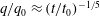 $q/q_{0}\approx (t/t_{0})^{-1/5}$
in the simulation with
$q/q_{0}\approx (t/t_{0})^{-1/5}$
in the simulation with
 $h_{1}/H=0.1$
(figure 10). In all three simulations, the bottom-propagating current transitions to a slumping phase, but the constant front velocity over this regime decreases slightly with increasing
$h_{1}/H=0.1$
(figure 10). In all three simulations, the bottom-propagating current transitions to a slumping phase, but the constant front velocity over this regime decreases slightly with increasing
 $h_{1}/H$
. In the simulation with
$h_{1}/H$
. In the simulation with
 $h_{1}/H=0.47$
, the front velocity of the bottom current starts decaying with time for
$h_{1}/H=0.47$
, the front velocity of the bottom current starts decaying with time for
 $|x_{f}/H|>12$
, which means the current leaves the slumping phase due to reduced discharge at
$|x_{f}/H|>12$
, which means the current leaves the slumping phase due to reduced discharge at
 $x/H=0$
.
$x/H=0$
.
The main effect of increasing the Reynolds number is to slightly increase the front velocity (e.g. by about 8–10 %). This is due to the increase of the front velocity with the Reynolds number for the part of the front situated within the intrusion layer (
 $\unicode[STIX]{x1D719}=0\,\%$
). However, once the transition to the drag-dominated regime is completed and drag forces largely dominate inertia forces, the difference between the front positions in the two cases remains close to constant in time (figure 9
c). For both cases,
$\unicode[STIX]{x1D719}=0\,\%$
). However, once the transition to the drag-dominated regime is completed and drag forces largely dominate inertia forces, the difference between the front positions in the two cases remains close to constant in time (figure 9
c). For both cases,
 $\unicode[STIX]{x1D6FC}=3/4$
. The front velocity of the bottom current during the slumping phase increases from
$\unicode[STIX]{x1D6FC}=3/4$
. The front velocity of the bottom current during the slumping phase increases from
 $0.41u_{b}$
to
$0.41u_{b}$
to
 $0.46u_{b}$
, which is close to the inviscid limit (
$0.46u_{b}$
, which is close to the inviscid limit (
 $0.5u_{b}$
) expected for lock-exchange currents propagating over a flat surface.
$0.5u_{b}$
) expected for lock-exchange currents propagating over a flat surface.
6 Flushing induced by the surface current
Convective flow driven by differences in water temperature plays an important role in the transport of nutrients and other substances between regions with and without vegetation (James & Barko Reference James and Barko1991; James, Barko & Eakin Reference James, Barko and Eakin1994; Zhang & Nepf Reference Zhang and Nepf2008). For floating vegetation, the residence time within the root (porous) layer is a critical parameter that can control the rate of nutrient uptake by roots, and the growth rate of floating vegetation. For example, when the biomass of hyacinth gets too high, which would be associated with a denser root zone, the growth rate declines (Imaoka & Teranishi Reference Imaoka and Teranishi1988). This might be explained by a decreased flushing rate associated with the denser root zone, which would limit the supply of nutrients. As the root zone becomes denser, the flushing rate declines, increasing the root zone residence time. If the root zone residence time becomes much longer that the uptake time scale, the nutrient uptake becomes supply limited, and overall uptake rate to the plant declines. Similarly, for water quality applications, the residence time of water within the porous (root) layer may control the overall nutrient removal from the water by both the roots and the biofilms existing on the root surfaces.
The residence time within the porous layer can be inferred from the time history of the volume of water with
 $C\leqslant 0.99$
advancing through the porous layer,
$C\leqslant 0.99$
advancing through the porous layer,
 $V$
. As the present investigation only considered cases in which the domain width,
$V$
. As the present investigation only considered cases in which the domain width,
 $W$
, and porous layer height,
$W$
, and porous layer height,
 $h_{1}$
, were constant, we consider the variable
$h_{1}$
, were constant, we consider the variable
 $V/(Wh_{1})$
, which has the dimension of a length, or its non-dimensional equivalent
$V/(Wh_{1})$
, which has the dimension of a length, or its non-dimensional equivalent
 $V/(HWh_{1})$
. Its slope characterizes the rate of streamwise advance (velocity) of lighter water through the porous layer, e.g. the rate at which new (lighter) water passes through the root layer (figure 11). Importantly, this quantity allows a more accurate estimation of the flushing time than the advection inferred from the velocity field within the porous layer, which would yield very long residence time, due to the near zero mean velocity in the porous layer in many cases (figure 5).
$V/(HWh_{1})$
. Its slope characterizes the rate of streamwise advance (velocity) of lighter water through the porous layer, e.g. the rate at which new (lighter) water passes through the root layer (figure 11). Importantly, this quantity allows a more accurate estimation of the flushing time than the advection inferred from the velocity field within the porous layer, which would yield very long residence time, due to the near zero mean velocity in the porous layer in many cases (figure 5).

Figure 11. Evolution of the normalized volume of heavier fluid removed by the surface current from the porous layer,
 $V/(h_{1}W)$
. The volume
$V/(h_{1}W)$
. The volume
 $V$
corresponds to the region with
$V$
corresponds to the region with
 $C<0.99$
inside the porous layer (
$C<0.99$
inside the porous layer (
 $x/H<0$
,
$x/H<0$
,
 $1-h_{1}<y/H<1$
). (a) Effect of solid volume fraction in the
$1-h_{1}<y/H<1$
). (a) Effect of solid volume fraction in the
 $Re=5758$
,
$Re=5758$
,
 $h_{1}/H=0.28$
simulations with
$h_{1}/H=0.28$
simulations with
 $\unicode[STIX]{x1D719}=8\,\%$
(light blue line),
$\unicode[STIX]{x1D719}=8\,\%$
(light blue line),
 $\unicode[STIX]{x1D719}=16\,\%$
(blue line) and
$\unicode[STIX]{x1D719}=16\,\%$
(blue line) and
 $\unicode[STIX]{x1D719}=24\,\%$
(black line); (b) effect of
$\unicode[STIX]{x1D719}=24\,\%$
(black line); (b) effect of
 $h_{1}/H$
in the (
$h_{1}/H$
in the (
 $Re=5758$
,
$Re=5758$
,
 $\unicode[STIX]{x1D719}=8\,\%$
) simulations with
$\unicode[STIX]{x1D719}=8\,\%$
) simulations with
 $h_{1}/H=0.1$
(orange line),
$h_{1}/H=0.1$
(orange line),
 $h_{1}/H=0.28$
(light blue line) and
$h_{1}/H=0.28$
(light blue line) and
 $h_{1}/H=0.47$
(green line); (c) effect of Reynolds number in the (
$h_{1}/H=0.47$
(green line); (c) effect of Reynolds number in the (
 $\unicode[STIX]{x1D719}=8\,\%$
,
$\unicode[STIX]{x1D719}=8\,\%$
,
 $h_{1}/H=0.28$
) simulations with
$h_{1}/H=0.28$
) simulations with
 $Re=5758$
(light blue line),
$Re=5758$
(light blue line),
 $Re=500\,000$
(red line).
$Re=500\,000$
(red line).
The rate of increase of the normalized volume of lighter water advancing through the porous layer,
 $V/(HWh_{1})$
, i.e. the flushing rate, increases with decreasing
$V/(HWh_{1})$
, i.e. the flushing rate, increases with decreasing
 $\unicode[STIX]{x1D719}$
(figure 11
a) and decreasing
$\unicode[STIX]{x1D719}$
(figure 11
a) and decreasing
 $h_{1}/H$
(figure 11
b). For relatively small values of
$h_{1}/H$
(figure 11
b). For relatively small values of
 $\unicode[STIX]{x1D719}$
and sufficiently low values of
$\unicode[STIX]{x1D719}$
and sufficiently low values of
 $h_{1}/H$
,
$h_{1}/H$
,
 $V/(HWh_{1})$
increases at close to linear rate with time (constant flushing rate), with
$V/(HWh_{1})$
increases at close to linear rate with time (constant flushing rate), with
 $V\sim t^{\unicode[STIX]{x1D6FD}}$
, and
$V\sim t^{\unicode[STIX]{x1D6FD}}$
, and
 $\unicode[STIX]{x1D6FD}=0.95$
for the
$\unicode[STIX]{x1D6FD}=0.95$
for the
 $h_{1}/H=0.1$
,
$h_{1}/H=0.1$
,
 $\unicode[STIX]{x1D719}=8\,\%$
case in figure 11(b). This result is not surprising given the close to linear increase of the front position with time (
$\unicode[STIX]{x1D719}=8\,\%$
case in figure 11(b). This result is not surprising given the close to linear increase of the front position with time (
 $\unicode[STIX]{x1D6FC}=0.95$
) for cases with a very thin porous layer (
$\unicode[STIX]{x1D6FC}=0.95$
) for cases with a very thin porous layer (
 $h_{1}/H=0.1$
,
$h_{1}/H=0.1$
,
 $\unicode[STIX]{x1D719}=8\,\%$
case in figure 9
b). For all other cases, the increase of
$\unicode[STIX]{x1D719}=8\,\%$
case in figure 9
b). For all other cases, the increase of
 $V/(HWh_{1})$
with time is less than linear and
$V/(HWh_{1})$
with time is less than linear and
 $\unicode[STIX]{x1D6FD}$
is slightly greater than
$\unicode[STIX]{x1D6FD}$
is slightly greater than
 $\unicode[STIX]{x1D6FC}$
(
$\unicode[STIX]{x1D6FC}$
(
 $=$
0.75). Only for the case where
$=$
0.75). Only for the case where
 $h_{1}/H$
is sufficiently high (
$h_{1}/H$
is sufficiently high (
 $h_{1}/H=0.47~\unicode[STIX]{x1D719}=8\,\%$
), such that most of the surface current is contained within the porous layer,
$h_{1}/H=0.47~\unicode[STIX]{x1D719}=8\,\%$
), such that most of the surface current is contained within the porous layer,
 $\unicode[STIX]{x1D6FD}=\unicode[STIX]{x1D6FC}=0.75$
. In the case with the largest
$\unicode[STIX]{x1D6FD}=\unicode[STIX]{x1D6FC}=0.75$
. In the case with the largest
 $\unicode[STIX]{x1D719}$
(e.g.
$\unicode[STIX]{x1D719}$
(e.g.
 $\unicode[STIX]{x1D719}=24\,\%$
,
$\unicode[STIX]{x1D719}=24\,\%$
,
 $h_{1}/H=0.28$
case in figure 11
a), the temporal variation of the rate of increase of
$h_{1}/H=0.28$
case in figure 11
a), the temporal variation of the rate of increase of
 $V/(HWh_{1})$
with time is non-monotonic. This is mainly because of the strong temporal variation in the distance between the front of the free-surface current in the porous layer and the front of the same current in the intrusion layer. The intrusions of lighter fluid into the porous layer in between the positions of the front of the free-surface current in the porous layer and in the intrusion layer are also contributing to the non-monotonic variation of the rate of increase of
$V/(HWh_{1})$
with time is non-monotonic. This is mainly because of the strong temporal variation in the distance between the front of the free-surface current in the porous layer and the front of the same current in the intrusion layer. The intrusions of lighter fluid into the porous layer in between the positions of the front of the free-surface current in the porous layer and in the intrusion layer are also contributing to the non-monotonic variation of the rate of increase of
 $V/(HWh_{1})$
. During the time intervals when the distance between the front positions in the two layers is relatively large, the rate of increase of
$V/(HWh_{1})$
. During the time intervals when the distance between the front positions in the two layers is relatively large, the rate of increase of
 $V/(HWh_{1})$
is high (
$V/(HWh_{1})$
is high (
 $\unicode[STIX]{x1D6FD}\approx 1$
). Finally, the effect of increasing the Reynolds number is felt only after the end of the transition to the drag-dominated regime (figure 11
c). As expected,
$\unicode[STIX]{x1D6FD}\approx 1$
). Finally, the effect of increasing the Reynolds number is felt only after the end of the transition to the drag-dominated regime (figure 11
c). As expected,
 $V/(HWh_{1})$
increases slightly faster in the higher Reynolds number case.
$V/(HWh_{1})$
increases slightly faster in the higher Reynolds number case.
As the discussion of the structure of the flow in §§ 3.1 and 3.2 has shown, the mean streamwise velocity inside the porous layer is small, suggesting that the renewal of water in the porous (root) layer would be minimal, especially for porous layers with large
 $\unicode[STIX]{x1D719}$
. However, the numerical results clearly show that the intrusion of less dense water from beneath the porous layer leads to significant convective mixing of fluid between the porous layer and the intrusion layer. This observation reveals the important, and previously unidentified, role of convective mixing and associated vertical exchange in setting the residence time of the root/porous layer. For example, for
$\unicode[STIX]{x1D719}$
. However, the numerical results clearly show that the intrusion of less dense water from beneath the porous layer leads to significant convective mixing of fluid between the porous layer and the intrusion layer. This observation reveals the important, and previously unidentified, role of convective mixing and associated vertical exchange in setting the residence time of the root/porous layer. For example, for
 $h_{1}/H=0.28$
and
$h_{1}/H=0.28$
and
 $\unicode[STIX]{x1D719}=8\,\%$
the residence time estimated from the velocity within the root layer is 6 times the actual flushing time estimated through the concentration fields (figure 11). This discrepancy increases with increasing solid volume fraction, such that for
$\unicode[STIX]{x1D719}=8\,\%$
the residence time estimated from the velocity within the root layer is 6 times the actual flushing time estimated through the concentration fields (figure 11). This discrepancy increases with increasing solid volume fraction, such that for
 $\unicode[STIX]{x1D719}=24\,\%$
the discrepancy is two orders of magnitude.
$\unicode[STIX]{x1D719}=24\,\%$
the discrepancy is two orders of magnitude.
The biological uptake by roots and biofilms takes place only in the root/porous layer. Using information from figure 11 on the variation of the normalized volume of lighter water advancing through the porous layer,
 $V/(HWh_{1})$
, before the end of the transition to the drag-dominated regime (
$V/(HWh_{1})$
, before the end of the transition to the drag-dominated regime (
 $t/t_{0}<30$
for most cases, see figures 9 and 10) together with the value of
$t/t_{0}<30$
for most cases, see figures 9 and 10) together with the value of
 $\unicode[STIX]{x1D6FD}$
one can estimate this variable at any time. This allows calculation of the length of the vegetated region that can be flushed in a typical day in real systems,
$\unicode[STIX]{x1D6FD}$
one can estimate this variable at any time. This allows calculation of the length of the vegetated region that can be flushed in a typical day in real systems,
 $L_{d}$
. Ultsch (Reference Ultsch1973) found that the average temperature difference between floating hyacinth and open water is about
$L_{d}$
. Ultsch (Reference Ultsch1973) found that the average temperature difference between floating hyacinth and open water is about
 $1^{\circ }\text{C}$
and persists for about 6 h each day (see figure 1–4 in Ultsch (Reference Ultsch1973). This temperature difference corresponds to a density difference of
$1^{\circ }\text{C}$
and persists for about 6 h each day (see figure 1–4 in Ultsch (Reference Ultsch1973). This temperature difference corresponds to a density difference of
 $0.25~\text{Kg}~\text{m}^{-3}$
. For typical applications, the mean water depth in the pond,
$0.25~\text{Kg}~\text{m}^{-3}$
. For typical applications, the mean water depth in the pond,
 $H$
, is about 1 m, the buoyancy velocity
$H$
, is about 1 m, the buoyancy velocity
 $u_{b}$
is
$u_{b}$
is
 $0.05~\text{m}~\text{s}^{-1}$
and the time scale
$0.05~\text{m}~\text{s}^{-1}$
and the time scale
 $t_{0}$
(
$t_{0}$
(
 $=H/u_{b}$
) is 20 s. If one assumes that the relative height of the root layer is
$=H/u_{b}$
) is 20 s. If one assumes that the relative height of the root layer is
 $h_{1}/H=0.28$
, then the value of
$h_{1}/H=0.28$
, then the value of
 $V/(HWh_{1})$
after 6 h (
$V/(HWh_{1})$
after 6 h (
 $t/t_{0}\approx 1100$
) is 95 for
$t/t_{0}\approx 1100$
) is 95 for
 $\unicode[STIX]{x1D719}=8\,\%$
and 60 for
$\unicode[STIX]{x1D719}=8\,\%$
and 60 for
 $\unicode[STIX]{x1D719}=24\,\%$
. These values were obtained using the values of
$\unicode[STIX]{x1D719}=24\,\%$
. These values were obtained using the values of
 $V/(HWh_{1})$
from the corresponding curves in figure 11(a) at
$V/(HWh_{1})$
from the corresponding curves in figure 11(a) at
 $t/t_{0}=60$
and then the assuming a power law variation
$t/t_{0}=60$
and then the assuming a power law variation
 $(V\sim t^{\unicode[STIX]{x1D6FD}})$
with the estimated values of
$(V\sim t^{\unicode[STIX]{x1D6FD}})$
with the estimated values of
 $\unicode[STIX]{x1D6FD}$
(
$\unicode[STIX]{x1D6FD}$
(
 ${\approx}$
0.78 for both
${\approx}$
0.78 for both
 $\unicode[STIX]{x1D719}=8\,\%$
and
$\unicode[STIX]{x1D719}=8\,\%$
and
 $\unicode[STIX]{x1D719}=24\,\%$
cases with
$\unicode[STIX]{x1D719}=24\,\%$
cases with
 $h_{1}/H=0.28$
) for
$h_{1}/H=0.28$
) for
 $60<t/t_{0}<1100$
. Then
$60<t/t_{0}<1100$
. Then
 $L_{d}=V(t=1,100t_{0}=6~\text{h})/(Wh_{1})$
. Using
$L_{d}=V(t=1,100t_{0}=6~\text{h})/(Wh_{1})$
. Using
 $H=1$
m, one obtains
$H=1$
m, one obtains
 $L_{d}=95$
m for
$L_{d}=95$
m for
 $\unicode[STIX]{x1D719}=8\,\%$
and
$\unicode[STIX]{x1D719}=8\,\%$
and
 $L_{d}=60$
m for
$L_{d}=60$
m for
 $\unicode[STIX]{x1D719}=24\,\%$
.
$\unicode[STIX]{x1D719}=24\,\%$
.
Ultsch’s (Reference Ultsch1973) measurements also suggest that the thermal exchange is only driven during heating, and during the night-time cooling there is negligible temperature difference. So, one could reasonably estimate a cumulative flushing over several days just from the day-time exchange for cases where the total length of the vegetated region,
 $L_{v}$
, (which might be of the order of tens to hundreds of meters in the field or treatment wetlands) is larger than
$L_{v}$
, (which might be of the order of tens to hundreds of meters in the field or treatment wetlands) is larger than
 $L_{d}$
. The root layer residence time can then be estimated as
$L_{d}$
. The root layer residence time can then be estimated as
 $T_{R}=Lv/L_{d}$
(days). Assuming a streamwise extent of about 50 m for the floating vegetation mats (Hill, Webb & Smith Reference Hill, Webb and Smith1987), our estimate for typical thermal conditions given above indicates that the thermal exchange can fully flush the root layer in one day. Wang & Sample (Reference Wang and Sample2014) described the uptake of phosphorus and nitrogen by floating mats of soft-stem bulrush (Schoenoplectus tabernaemontani) and pickerel weed (Pontederia cordata L.) by a first-order reaction with first-order rate constants of
$T_{R}=Lv/L_{d}$
(days). Assuming a streamwise extent of about 50 m for the floating vegetation mats (Hill, Webb & Smith Reference Hill, Webb and Smith1987), our estimate for typical thermal conditions given above indicates that the thermal exchange can fully flush the root layer in one day. Wang & Sample (Reference Wang and Sample2014) described the uptake of phosphorus and nitrogen by floating mats of soft-stem bulrush (Schoenoplectus tabernaemontani) and pickerel weed (Pontederia cordata L.) by a first-order reaction with first-order rate constants of
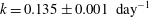 $k=0.135\pm 0.001~\text{day}^{-1}$
(phosphorus) and
$k=0.135\pm 0.001~\text{day}^{-1}$
(phosphorus) and
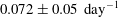 $0.072\pm 0.05~\text{day}^{-1}$
(nitrogen). These rates correspond to uptake reaction time scales,
$0.072\pm 0.05~\text{day}^{-1}$
(nitrogen). These rates correspond to uptake reaction time scales,
 $T_{k}=1/k$
, of approximately 7–14 days. Since in our example
$T_{k}=1/k$
, of approximately 7–14 days. Since in our example
 $T_{R}<T_{k}$
, the flushing can significantly enhance the overall rate of nutrient removal by maintaining higher concentration of nutrient with the root zone. Though in our example the exchange flow can fully flush the area each day that may not be the case when the average temperature difference is smaller.
$T_{R}<T_{k}$
, the flushing can significantly enhance the overall rate of nutrient removal by maintaining higher concentration of nutrient with the root zone. Though in our example the exchange flow can fully flush the area each day that may not be the case when the average temperature difference is smaller.
7 Summary and conclusions
Highly resolved, 3-D LES were used to study the effects of a surface porous layer present on one side of a lock gate on the long-term evolution of the lock-exchange flow. This problem was motivated by thermally driven exchange between open water and a region containing floating vegetation. For all cases there is a net mass exchange within the surface current, between the porous layer and the intrusion layer beneath. Near the lock gate, fluid is advected downward from the porous layer into the intrusion layer, while the opposite happens close to the front (figure 1). Moreover, for sufficiently high values of
 $\unicode[STIX]{x1D719}$
, most of the flow leaves the porous layer close to origin (leading edge of the porous layer) and a region of negligible velocity within the porous layer forms until the head region is approached. For high porous layer heights (
$\unicode[STIX]{x1D719}$
, most of the flow leaves the porous layer close to origin (leading edge of the porous layer) and a region of negligible velocity within the porous layer forms until the head region is approached. For high porous layer heights (
 $h_{1}/H>0.4$
), the structure of the surface current resembles that observed in the fully vegetated case (e.g. the interface inside the porous region varies linearly with the distance from the front, starting some distance away from the front).
$h_{1}/H>0.4$
), the structure of the surface current resembles that observed in the fully vegetated case (e.g. the interface inside the porous region varies linearly with the distance from the front, starting some distance away from the front).
For sufficiently high values of the
 $\unicode[STIX]{x1D719}$
and
$\unicode[STIX]{x1D719}$
and
 $h_{1}/H$
, the surface current transitions to a quadratic-drag-dominated regime in which the front velocity is proportional to
$h_{1}/H$
, the surface current transitions to a quadratic-drag-dominated regime in which the front velocity is proportional to
 $t^{-1/4}$
, and the discharge at the lock gate position decays proportional to
$t^{-1/4}$
, and the discharge at the lock gate position decays proportional to
 $t^{-1/3}$
. Both results are similar to those obtained by Ozan et al. (Reference Ozan, Constantinescu and Hogg2015) for the fully vegetated case. The decreasing discharge within the surface current also caused the velocity of the bottom current, advancing into a region with zero
$t^{-1/3}$
. Both results are similar to those obtained by Ozan et al. (Reference Ozan, Constantinescu and Hogg2015) for the fully vegetated case. The decreasing discharge within the surface current also caused the velocity of the bottom current, advancing into a region with zero
 $\unicode[STIX]{x1D719}$
, to decay with time. Even in cases for which a region with negligible flow velocities developed within the porous layer and the flow in the two layers was far from horizontal, the front velocity decayed proportional to
$\unicode[STIX]{x1D719}$
, to decay with time. Even in cases for which a region with negligible flow velocities developed within the porous layer and the flow in the two layers was far from horizontal, the front velocity decayed proportional to
 $t^{-1/4}$
, provided that
$t^{-1/4}$
, provided that
 $h_{1}/H$
was sufficiently high. For cases with a small
$h_{1}/H$
was sufficiently high. For cases with a small
 $h_{1}/H$
, most of the surface current propagates through the intrusion layer, and the decay of the front velocity is weaker (smaller power law coefficient) compared to cases with deeper
$h_{1}/H$
, most of the surface current propagates through the intrusion layer, and the decay of the front velocity is weaker (smaller power law coefficient) compared to cases with deeper
 $h_{1}/H$
.
$h_{1}/H$
.
The simulations revealed the details of an unstable stratified region that develops at the interface between the porous and intrusion layers due to the difference in the velocity within the two layers. Especially for cases with a large
 $\unicode[STIX]{x1D719}$
, the removal of the heavier fluid from the porous layer is driven by convective exchange with lighter fluid originating in the intrusion layer (figure 3). As a result, 2-D effects are important and the flow within the porous and intrusion layer is far from being unidirectional. This means that the utility of shallow-water theory to predict the front velocity and other flow variables for the present three-layer problem is questionable.
$\unicode[STIX]{x1D719}$
, the removal of the heavier fluid from the porous layer is driven by convective exchange with lighter fluid originating in the intrusion layer (figure 3). As a result, 2-D effects are important and the flow within the porous and intrusion layer is far from being unidirectional. This means that the utility of shallow-water theory to predict the front velocity and other flow variables for the present three-layer problem is questionable.
The numerical results illustrate how the root zone is flushed by a combination of the advancing intrusion layer and the vertical exchange between the intrusion layer and the porous layer. The residence time of the root zone was estimated by tracking the volume of lighter fluid inside the porous layer, and in most cases this true residence was much shorter (in some cases by two orders of magnitude) than what would be estimated from the velocity within the root zone, highlighting the importance of the vertical exchange. Estimates of root zone residence time in field conditions suggests that the flushing of the root zone by thermally driven exchange currents can significantly enhance to the uptake of nutrients by the root system.
Acknowledgements
We gratefully acknowledge the National Center for High Performance Computing (NCHC) in Taiwan, in particular Dr W. F. Tsai, and the Transportation Research and Analysis Computing Center (TRACC) at the Argonne National Laboratory, in particular Dr S. Lottes, for providing substantial computer time. A.Y.-O. acknowledges financial support through the Scientific and Technological Research Council of Turkey (TUBITAC) for post-doctoral research fellowship.
Supplementary movies
Supplementary movies are available at https://doi.org/10.1017/jfm.2016.698.


