I

In this article we re-evaluate the hypothesis that bank lending was a key factor in the growth process in nineteenth-century Germany and that it was instrumental in financing the industrial revolution. This hypothesis has been developed, among others, by the influential economic historian Alexander Gerschenkron (Reference Gerschenkron1962). This conventional view has been adopted by most researchers and has triggered a literature that discusses the benefits of close relationships between banks and firms that were said to be typical of Germany at the time. A survey of papers arguing along these lines is given, for instance, in Guinnane (Reference Guinnane2002). A notable exception, however, is Edwards and Ogilvie (Reference Edwards and Ogilvie1996), who challenge this view and point out that large universal banks that serviced the big industrial firms contributed only a small fraction to total bank lending. They argue that universal banks were primarily engaged in organising the issuance of new shares, but hardly contributed to financing long-term investment by credit.

We employ a new data set to reinvestigate whether there has been a positive effect of bank lending on growth and whether indeed the industrial sector – or possibly other sectors in the economy – benefited most strongly from the development of domestic credit in Germany. This data set was initially compiled by Walther Hoffmann (Reference Hoffmann1965) for the sample period of 1870–1912 and includes a detailed sectoral disaggregation of output.Footnote ² It therefore allows us to trace the effect of the rapid increase in bank lending on net domestic product, as well as on the sectoral structure underneath it.Footnote ³ In our article, we focus on the main subsectors, mining, industry, construction, agriculture, transportation, trade and services.

In the empirical analysis, we use a VAR framework to trace the effect of an unexpected shock in aggregate lending on domestic product and its subsectors. From the VAR coefficients, we generate impulse response functions in two different ways. On the one hand, we use generalised impulse response functions. These can be computed without prior knowledge of the contemporaneous causal relationships among the variables. On the other hand, we use a Cholesky decomposition that was proposed by Tornell and Westermann (Reference Tornell and Westermann2005) and that, using an appropriate ordering, can be interpreted as structurally identified in the context of a theoretical two-sector growth model with credit market imperfections. As output, in the model, depends on investment and credit in period t-1, it is assumed not to be affected by bank lending in the same period.Footnote ⁴

Considering first the aggregate variables, we find that net domestic product (NDP) displays a significant and positive reaction to a standard shock in the bank lending variable, using both identification approaches. We find a direct effect on NDP and an additional indirect channel via its effect on investment. This finding is consistent with most papers on economic history (see, for instance, Burhop (Reference Burhop2006) for Germany, Levine (Reference Levine1997), King and Levine (Reference King and Levine1993), Rousseau and Wachtel (Reference Rousseau and Wachtel1998, Reference Rousseau and Wachtel2000) and Schularick and Steger (Reference Schularick and Steger2010) for other countries), as well as a large body of literature on finance and growth in the post-World War II period, in particular in today's emerging markets (see Beck et al. (Reference Beck, Levine and Loayza2000) for an overview).

In the sectoral analysis, we find that all subsectors also react significantly to an unexpected shock in aggregate lending. It is interesting, however, that the importance of these shocks varies substantially across sectors. In a variance decomposition of the forecast errors, we find that for the mining sector, the industrial sector and the trade sector, shocks from the banking system only play a minor role. The agricultural sector, the construction sector, the transportation sector and the service sector, on the other hand, are substantially more affected. Although our findings confirm previous empirical studies on the aggregate impact of bank lending on growth, they therefore challenge the conventional view of the role the banking system has actually played in promoting growth. Our results indicate that rather than speeding up the structural change within the industrial sectors, the importance of bank lending was that it allowed other sectors to keep pace. In a period of rapid technological change, it seems to have allowed for a more balanced growth path than could otherwise have taken place. This result appears to be at odds with the hypothesis that the industrial sector benefited most from the development of lending in the banking sector, but is consistent with Edwards and Ogilvie's view that the German banking system was primarily engaged in small-firm financing.

The importance of sectoral information, when analysing the effects of financial deepening on growth, has also been emphasised in Tornell and Schneider (Reference Tornell and Schneider2004), who point out that aggregate measures on output often mask deep sectoral asymmetries in credit-constrained economies.Footnote ⁵ It is interesting that the sectoral patterns observed in today's emerging markets are indeed reminiscent of the sectoral growth patterns in nineteenth-century Germany. Tornell, Westermann and Martinez (Reference Tornell, Westermann and Martinez2003) have documented in a broad cross-section of middle-income countries from 1980 to 2000 that there exists a pronounced shift towards small firms and those producing non-tradable goods in periods of rapid credit expansion.Footnote ⁶ Tornell and Schneider (Reference Tornell and Schneider2004) motivate theoretically that small firms in non-tradable-goods-producing sectors are likely to benefit most from bank lending, while the tradable sectors typically consist of large firms that have other forms of financial instruments available. In their model, the latter sectors can borrow directly from the (international) capital market and are largely unaffected by the domestic banking system. Taking into account these characteristics of credit markets, Rancière and Tornell (Reference Rancière and Tornell2010) developed a two-sector growth model, in which the non-tradable sector creates a ‘bottleneck’ to economic growth as it is used as an input in the tradable sectors' production. Relaxing the credit constraints in the non-tradable sector therefore leads to overall higher growth.

The empirical results in our article seem to confirm this view. The industrial, mining and trade sectors are classical tradable-goods-producing sectors. In particular, the industrial sector displayed the highest export share during the late nineteenth and early twentieth century in Germany. Also the latter two sectors consist of mostly large firms. Construction, transportation and services, on the other hand, are clearly non-tradable. Although agriculture ranks among the more tradable sectors today, it is plausible that due to the lack of modern refrigeration technologies as well as high tariffs, its output was substantially less tradable more than a century ago. Also, this sector is characterised by a large number of relatively small firms.Footnote ⁷

The rapid increase in productivity of small agricultural firms is documented in van Zanden (Reference Van Zanden1991).Footnote ⁸ Its importance for the industrial revolution has been discussed for instance in Perkins (Reference Perkins1981) and Webb (Reference Webb1982).Footnote ⁹ In the context of the Rancière and Tornell model, it can be seen as an input into the production process, and the financial sector development helps to remove this bottleneck that prevents an overall higher growth path. Finally, the assumptions on credit market imperfection in the Tornell and Schneider (Reference Tornell and Schneider2004) model are likely to be valid for our sample period. Guinnane (Reference Guinnane2001) has argued that rural credit was a significant problem in nineteenth-century Germany and pointed out that ‘credit conditions in Germany sound similar to those found in many developing countries today’ (p. 368).

We test for the robustness of our results in several ways. First, we employ three alternative indicators of bank lending, the net contribution of banks to financing investment and total assets in the banking system, reported by Hoffmann (Reference Hoffmann1965), as well as the total assets of joint-stock credit banks, reported by Burhop (Reference Burhop2002) and Deutsche Bundesbank (1976). Furthermore, we use data on equity capital to show that the non-tradable sectors did not benefit disproportionately from the alternative forms of financing that are typically used by large industrial firms. When using equity capital in our VARs instead of bank lending, the industrial sector is the one that reacts to an unexpected increase in financial resources most strongly.

Section II provides a description of the dataFootnote ¹⁰ and a preliminary analysis of the unit root and cointegration properties. The VAR analysis of aggregate output is given in Section III. Section IV contains the sectoral analysis and robustness tests. Section V concludes.

II

The data in our analysis are drawn from a book written by the German economic historian Walther Hoffmann (Reference Hoffmann1965). This data set is particularly useful for our analysis because it includes a detailed decomposition of sectoral output.

Our main variables are the net domestic product (NDP),Footnote ¹¹ investment (I)Footnote ¹² and bank lending (B).Footnote ¹³ Both domestic product and investment are expressed in net terms and in constant 1913 prices. Our bank variable captures the contribution of banks in the financing of net investment.

On a disaggregated level we consider the following sectors: mining (M), industry (IN), agriculture (A), trade (T), transportation (TR) and services (S).Footnote ¹⁴ The mining sector contains value added of mining and salines, the industry sector consists of industry and skilled crafts, and the agriculture sector covers the value added of farming, forest and fisheries. The trade sector contains the value added of trade, banks, insurances and public houses. Figure 1 shows the time paths of the sectors in logged terms. While mining and industrial production were growing very fast over our sample period there was also substantial growth in agriculture. Transportation was the fastest growing among all sectors.

Figure 1. Sectoral output growth (in logs)

Note: The graphs for the sectoral output of mining (M), industry (IN), agriculture (A), trade (T), transportation (TR), and services (S) are displayed.

We also take an alternative measure of the banks' contribution to financing investment. Our indicator total assets 1 (TA1) includes the total assets of savings banks, cooperative credit associations, mortgage banks, banks of issue, land mortgage banks and commercial banks.Footnote ¹⁵Total assets 2 (TA2) represents the total assets of joint-stock credit banks reported in Burhop (Reference Burhop2002). The variable equity capital (EC) represents the paid-up capital of stock corporations.Footnote ¹⁶ All data are recorded on an annual basis. The sample period covers the years 1870–1912.Footnote ¹⁷

We start our empirical analysis by testing the unit root properties of our time series. We first apply the conventional Augmented Dickey Fuller test. In Table 1, which reports the results for our main variables, we can see that all of our time series are nonstationary in levels, but stationary in first differences. The optimal lag length in the test specifications was chosen by the Schwarz information criterion.

Table 1. Results of the ADF tests

Note: The ADF test is calculated for levels and first differences for the variables net domestic product (NDP), investment (I), bank lending (B), total assets 1 (TA1), total assets 2 (TA2), equity capital (EC), mining (M), industry (IN), agriculture (A), trade (T), transportation (TR) and services (S) for the years 1870–1912. The lag length is selected by the Schwarz information criterion. *** indicates significance at the 1% level.

In the following sections of the article we will estimate the causal linkages among our main variables by using a vector autoregression. In this VAR our variables enter in logged levels and we therefore need to check the cointegration properties of our data set as a second preliminary exercise (see Table 2).

Table 2. Results of cointegration tests

Note: * and ** indicate significance at 5% and 1% level by employing critical values from Osterwald-Lenum. ° and °° indicate significance at 5% and 1% level for critical values from Cheung and Lai (Reference Cheung and Lai1993). For Engle and Granger (Reference Engle and Granger1987) cointegration, * and ** indicate significance at 5% and 1% level using critical values from MacKinnon (Reference Mackinnon, Engle and Granger1991).

Overall, there is substantial evidence on cointegration among our time series, although in some cases the evidence is mixed, when using different techniques of estimation. Using the Engle and Granger (Reference Engle and Granger1987) approach, we find evidence of cointegration among all pairs of time series that later enter the VAR analysis, except services and bank lending. We cannot generally confirm cointegration using the Johansen (Reference Johansen1991) test, however. In particular, the three-variable system of net domestic product, investment and bank lending as well as some bivariate combinations do not appear cointegrated in this second approach.

Although there is only mixed evidence on cointegration, we continue with the VAR specification in levels, as the alternative – an estimation in first differences – seems to have even more severe shortcomings. The time series in the first differences have a much higher variance at the beginning of the sample than towards the end. The intuition of this phenomenon is that at this very early stage of development, the time series start to grow from very low levels. Thus, positive as well as negative growth rates will have a much larger amplitude than in the later part of the sample, where they have reached a higher level.

Proceeding with the VAR in levels, we need to keep in mind, however, a potential bias in our results if the time series are not clearly cointegrated. Except for the bivariate combination of services and bank lending, we can reject the null of no cointegration in at least one of the three approaches (Engle/Granger, Johansen, Trace/Max-Eigenvalue Statistic).

III

In the subsequent analysis, we take two different approaches to modelling the link between financial development and growth. One of the key issues in a VAR framework is the identification of structural shocks. In our first approach, we apply the concept of generalised impulse responses. This approach has the benefit that the impulse response functions are independent of the ordering of the variables in the VAR. Its drawback, however, is that the structural shocks are ultimately not identified. We simulate a system shock, where the contemporaneous reactions of the other variables are already included.

In the second approach we follow the structural identification proposed in Tornell and Westermann (Reference Tornell and Westermann2005). In this article, the identification is based on a theoretical two-sector growth model that also guides the analysis in the later sections of the article. We employ a Cholesky decomposition, where output cannot contemporaneously react to domestic lending in the same period. The intuition is that output results from investment that is financed by domestic credit in the period t-1. This also applies to sectoral output. As lending, on the other hand, can react to changes in output in the same period, we have a recursive system that can be used to identify shocks from each variable, following the standard Cholesky procedure. The advantage of this approach is that a structural interpretation can be given to the impulse response functions in the context of this model. A drawback is that we need to limit the analysis to bivariate systems. In our view, neither of the two approaches may clearly be better, but jointly, they give a more complete picture of the link between financial development and growth.

Generalised impulse response functions

Figure 2 reports the generalised impulse responses from our first VAR, which includes the variables net domestic product, investment and bank lending. Our main interest is in the effect that banks have on the net domestic product, which is displayed in panel A. There, a statistically significant effect for about four years exists. Panel B shows that there is in addition another indirect effect. For a period of three to four years, an unexpected increase in bank lending increases investment. It is well known that investment, in turn, has a positive impact on NDP.Footnote ¹⁸

Figure 2. Generalized impulse responses for net domestic product, investment and bank lending

Note: The solid lines trace the impulse responses of net domestic product (NDP) and investment (I) to shocks in bank lending (B) for the years 1870–1912.

Although the impulse response functions have revealed a clear link between aggregate bank credit and net domestic product, they do not allow us to assess the importance of these shocks in the total forecast error variance. For this purpose, we conduct a variance decomposition as a next step. Table 3 shows the variance decomposition for a forecast horizon of five and ten years. We find that bank lending explains up to 24 per cent of the forecast error variance of net domestic product and up to 30 per cent of the forecast error variance of investment. Although this implies that others shocks seem to be more important, this is a relatively high number in a VAR analysis.Footnote ¹⁹

Table 3. Variance decomposition for net domestic product, investment and bank lending

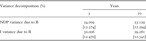
Note: The variance decomposition of the forecast error is shown for the three-variable VAR, including net domestic product (NDP), investment (I) and bank lending (B) for the years 1870–1912. The values in parentheses indicate the standard deviation.

Cholesky decompositions

In this section, we estimate the alternative approach of a Cholesky decomposition (see Tornell and Westermann (Reference Tornell and Westermann2005)). Panel A and panel B of Figure 3 show the results of the impulse response functions, generated from two different VARs. In this first VAR, we only include net domestic product (NDP) and bank lending (B); in the second one, we include NDP and investment (I). Panel A shows that there is a positive and significant reaction of net domestic product to an unexpected shock in bank lending. Furthermore, in panel B, we see that there is also a significant reaction of investment to bank lending.Footnote ²⁰ The variance decomposition, reported in Table 4, shows that the shock in bank lending explains 21 per cent and 25 per cent of the forecast error variance. Thus, the results seem to confirm the finding from the previous section that used generalised impulse response functions.

Figure 3. Impulse responses for net domestic product and bank lending, and investment and bank lending

Note: The solid lines trace the impulse responses of net domestic product (NDP) and investment (I) to shocks in bank lending (B) for the years 1870–1912.

Table 4. Variance decomposition for net domestic product and bank lending, and investment and bank lending

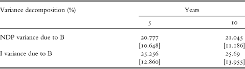
Note: The variance decomposition of the forecast error is shown for the two-variable VARs, including net domestic product (NDP) and bank lending (B), and investment (I) and bank lending (B) for the years 1870–1912. The values in parentheses indicate the standard deviation.

IV

The findings in the previous sections largely confirmed earlier research on historical data in Germany and other countries. A key question that we would like to address in the present article is to understand which sectors of the economy benefited most from the positive link between bank lending and growth. In the literature on today's emerging markets, pronounced sectoral asymmetries are often found, and we find it very interesting to compare how the growth process in nineteenth-century Germany relates to the experiences of the emerging markets of the last 20 to 30 years. We therefore also investigate the sectoral differences in the responses of output to aggregate lending in this section.

In the literature on financial development in emerging markets, sectors are typically classified as small (and non-tradable) or large (and tradable). The motivation for this classification is that the former set of firms finances investment mainly via the domestic banking system, while the latter has other financial instruments available, such as issuing equity or commercial paper, or borrowing on the international capital market. It is often found that the strength of the link between financial development and output growth differs substantially between these two groups. This difference across sectors is quite pronounced in middle-income countries and emerging markets but less prevalent in industrial economies.

The data set of Hoffmann (Reference Hoffmann1965) includes detailed information on the sectoral aggregate accounts of Germany and allows us to perform such a decomposition. We focus on six main subsectors of NDP, the industrial sector, mining, agriculture, trade, transportation and services.

Figure 4 shows the impulse response functions that were generated from bivariate VARs, including the respective measure of output and our bank lending variable. As in the previous section, we generate the impulse response functions from a Cholesky decomposition, where the bank lending variable is ordered at the second position in the VAR.

Figure 4. Impulse responses for sectoral output and bank lending

Note: The solid lines trace the impulse responses of the sectoral output of mining (M), industry (IN), agriculture (A), trade (T), transportation (TR) and services (S) to a shock in bank lending (B) for the years 1870–1912.

We find that in all sectors there is a positive reaction of output to an unexpected shock in bank lending. In all sectors, except for the trade sector, this reaction is also statistically significant at the 5 per cent level.Footnote ²¹ However, the variance decomposition in Table 5 shows that the shocks coming from the banking system are of quite different importance for the various sectors of the economy. The insignificant trade sector is least affected by banks. Shocks from the banking system explain only up to 4.9 per cent of the forecast uncertainty of the trade sector. Interestingly, shocks from the banking system also show little impact on the industry and mining sectors, with values of 9.3 per cent and 5.7 per cent. This finding is interesting as it challenges the conventional wisdom that the industrial revolution was substantially accelerated by the parallel development of the banking system. On the other hand, we find that the sectors most affected by shocks in the banking system were agriculture (up to 17.9 per cent), transportation (up to 25.5 per cent) and services (up to 25 per cent).Footnote ²²

Table 5. Variance decomposition for sectoral output and bank lending

Note: The variance decomposition (in percent) is shown for the sectoral output of mining (M), industry (IN), agriculture (A), trade (T), transportation (TR) and services (S). The figures show the share of the forecast error variance that is due to a shock in bank lending (B).

The structure of German exports – that was also recorded, although not on an annual basis, by Hoffmann (Reference Hoffmann1965) – suggests that the industrial sector was indeed the most tradable in Germany. In 1910–13, final goods had the largest share in total German exports – textiles (12.3 per cent), metal and machinery (21 per cent) as well as chemicals (9.9 per cent) – followed by raw materials such as coal (5.3 per cent) and half-manufactured goods such as iron (6.6 per cent). Food products, such as grain (3.4 per cent) and sugar (2.3 per cent), had substantially smaller shares.Footnote ²³ Exports as a share of production were also quite high within some sectors. The highest shares were recorded for leather products (110 per cent), metal products (93 per cent) and textiles (99 per cent) in 1910–13. Overall the export share of production increased from 70 per cent in 1875–9 to 95 per cent in 1910–13.Footnote ²⁴

Although this evidence does not support the view that bank development was very important for the technological progress that occurred in manufacturing during the industrial revolution, it is remarkable that the patterns in nineteenth-century Germany are very similar to modern emerging markets. In emerging markets it is typically found that the non-tradable sectors are impacted the most by the domestic banking system (see Tornell and Westermann (Reference Tornell and Westermann2005) and IMF (2003)). Table 5 shows that this was also the case in nineteenth-century Germany, as both services and transportation are clearly non-tradable. Due to the lack of modern refrigeration, the output of the agricultural sector is likely to have been relatively non-tradable as well. Webb (Reference Webb1977) documents that tariff protection was substantially higher in agriculture than in other industrial sectors.

Bank lending measured by total assets

In this subsection we perform some robustness tests on our main findings that (a) banks contributed substantially to investment and growth in nineteenth-century Germany and (b) this has been particularly important for non-tradable sectors. We start by taking an alternative measure of bank lending.

As all of our variables – net domestic product and investment – are in net terms, we initially started the analysis with the net contribution of the banking system to financing investment as our main indicator of bank lending. In the present section we first take the more conventional measure of total assets in the banking system that is also reported in the Hoffmann data set as an alternative (denoted as TA1 in the following tables).

The impulse response functions of the six sectors of the economy are displayed in Figure 5. We see that all sectors (except trade) respond positively to a standard shock in our alternative measure of bank lending.Footnote ²⁵Table 6 shows, furthermore, that we find roughly similar results also for the variance decomposition. Overall the share of the forecast error variance is somewhat higher than in the previous tables. The least affected sector is still the trade sector (up to 7.3 per cent), followed by the industrial sector (24.8 per cent), mining (32.1 per cent) and transportation (33.9 per cent). Substantially higher values are found in the agricultural sector (53.3 per cent) and in services (59.9 per cent). Again, the non-tradable sectors appear to have been more strongly affected by bank lending than the industrial or mining sector.

Figure 5. Impulse responses for sectoral output and total assets 1

Note: The solid lines trace the impulse responses of the sectoral output of mining (M), industry (IN), agriculture (A), trade (T), transportation (TR) and services (S) to a shock in total assets 1 (TA1) for the years 1870–1912.

Table 6. Variance decomposition for sectoral output and total assets 1

Note: The variance decomposition (in percent) is shown for the sectoral output of mining (M), industry (IN), agriculture (A), trade (T), transportation (TR) and services (S). The figures show the share of the forecast error variance that is due to a shock in total assets 1 (TA1).

Furthermore, we compare our findings to a second measure of total assets, reported by Burhop (Reference Burhop2006) and Deutsche Bundesbank (1976) (denoted as TA2). This second measure of total assets is restricted to the assets of joint-stock credit banks, but has been used in earlier studies, including Burhop (Reference Burhop2002) who updated the data set until 1913.Footnote ²⁶

An alternative measure of total assets

In this second measure of total assets (TA2), we again find a positive and significant response of output in all sectors to an unexpected change in lending, as documented in Figure 6.Footnote ²⁷ In Table 7, we see that there are substantial differences in the variance decomposition. The largest responses are in the agricultural and service sectors, where the responses are statistically significant at the 5 per cent level. Among the remaining sectors, lending seems to be least important for the trade sector, followed by industry, mining and transportation. In all these sectors, the share of the variance that can be explained by shocks from the banking system is statistically insignificant after ten years. Overall these patterns are quite similar to the previous bank lending measures.

Figure 6. Impulse responses for sectoral output and total assets 2

Note: The solid lines trace the impulse responses of the sectoral output of mining (M), industry (IN), agriculture (A), trade (T), transportation (TR) and services (S) to a shock in total assets 2 (TA2) for the years 1870–1912.

Table 7. Variance decomposition for sectoral output and total assets 2

Note: The variance decomposition (in percent) is shown for the sectoral output of mining (M), industry (IN), agriculture (A), trade (T), transportation (TR) and services (S). The figures show the share of the forecast error variance that is due to a shock in total assets 2 (TA2).

Equity capital

Finally, we perform a plausibility test for our main hypothesis that small, non-tradable-goods-producing sectors were dependent on the banking system, while other sectors, in particular the industrial sector, had other sources of finance available. In the Hoffmann data set, we extracted the time series on total equity capital (denoted as equity capital (EC)) that was raised in the economy by listed stock market companies. When we use this indicator in our regressions – instead of bank lending – we find that the industrial sector does indeed show the strongest reaction to an unexpected change in equity capital that is statistically significant at the 5 per cent level (see Figure 7). Most other sectors (except mining) also show a significant but quantitatively smaller reaction than the industrial sector.Footnote ²⁸ When looking at the variance decomposition Table 8, this finding is also confirmed. After five years, the industrial sector and the trade sector show the highest share of forecast error variance that is explained by the equity shocks with 20.5 per cent and 23.4 per cent, respectively. After a period of ten years, it is again the agricultural sector that is most affected, followed by the industrial sector and the trade sector, although with a much smaller lead compared to the previous section. For services the equity financing plays a much smaller role, explaining only 5.2 per cent of the variance after five years and 11.1 per cent after ten years.

Figure 7. Impulse responses for sectoral output and equity capital

Note: The solid lines trace the impulse responses of the sectoral output of mining (M), industry (IN), agriculture (A), trade (T), transportation (TR) and services (S) to a shock in equity capital (EC) for the years 1870–1912.

Table 8. Variance decomposition for sectoral output and equity capital

Note: The variance decomposition (in percent) is shown for the sectoral output of mining (M), industry (IN), agriculture (A), trade (T), transportation (TR) and services (S). The figures show the share of the forecast error variance that is due to a shock in equity capital (EC).

Sectoral output data by Burhop/Wolff and further robustness tests

In a further robustness test, we investigate an alternative sectoral data set that was used by Burhop and Wolff (Reference Burhop and Wolff2005) and Burhop (Reference Burhop and Wolff2005). In this alternative data set, we are able to confirm that the industrial sector reacts more strongly to equity capital than to bank lending. Figure 8 shows that the industrial sector's reaction to bank lending is statistically insignificant while the reaction to equity capital is significant for three to ten years. The construction sector, on the other hand, reacts more strongly to changes in bank lending. The reaction is statistically significant and Table 9 shows that shocks coming from the banks explain a substantial share of the total forecast error variance. In the variance decomposition of the industrial sector, we see that the share explained by equity capital is substantially larger than the share explained by banks.

Figure 8. Impulse responses for industry 2 and construction to shocks in bank lending and equity capital

Note: The solid lines trace the impulse responses for industry 2 (IN2) and construction (C) to shocks in bank lending (B) and equity capital (EC) for the years 1870–1912.

Table 9. Variance decomposition for industry 2 and construction to shocks in bank lending and equity capital

Note: The variance decomposition (in percent) is shown for industry 2 (IN2) and construction (C). The figures show the share of the forecast error variance that is due to a shock in bank lending (B) and equity capital (EC).

We have implemented several further robustness tests to our main specification. The results are available upon request. In particular, we have extended the VAR to include further control variables, such as interest rates, money and prices. Of course there are some differences in the details but overall the findings reported in this article remain quite robust. An advantage of a larger specification is that in a full system, the long-term effects become insignificant reflecting the long-term neutrality of money and credit. However, the VAR specification also suffers from an increasingly severe identification problems and larger standard errors due to the relatively small sample period.

V

In this article we attempted to evaluate the role that the banking system played in nineteenth-century Germany by taking a sectoral perspective. We found evidence that the sectors of the economy were affected asymmetrically by shocks from bank lending. This evidence is robust to reasonable alternative estimation procedures and alternative indicators of bank lending. Our central finding is that it was not the industrial sector, but transportation, agriculture, services and construction that benefited most from the development of the banking sector.

We explain this new stylised fact, referring to a two-sector growth model of Tornell and Schneider (Reference Tornell and Schneider2004), who show that small, non-tradable-goods-producing firms benefit most from lending booms in economies with contract-enforceability problems. We point out that our findings are indeed similar to stylised facts that have been documented on today's emerging markets. During boom–bust cycle episodes in the 1980s and 1990s, the non-tradable sector has often grown more strongly during the boom phase and fallen into a more deep and sustained recession in the aftermath of banking crisis.

Several questions remain unanswered, however, that further research might be able to address. First, we found that – similar to today's emerging markets – the tradable sector was hardly affected by domestic banks. But was this due to a well enough developed international capital market, or due to the size of the firms in the industrial sector, which had equity finance and other domestic financial instruments available? The Hoffmann data set gives some indication that capital markets were indeed quite open. German gross foreign assets increased, for instance, from 7,172 million Mark in 1882 to 19,396 million Mark in 1912. The foreign emissions of equity and commercial paper increased from 300 million Mark in 1883 to 604 million Mark in 1913 (with a peak of 1,108 million Mark in 1905).Footnote ²⁹ Also the trade account appears to have been quite open, as between 1880 and 1913 the share of exports to NDP fluctuated between 12.8 per cent and 17.7 per cent.Footnote ³⁰ The openness of financial markets in the nineteenth century has also been documented by Bordo (Reference Bordo2002). In addition, it is worth noting that changes in the tariffs on different sectors might have affected the asymmetries in sectoral growth patterns.

Furthermore, there may have been other influences on the agricultural sector in particular. Institutional barriers in the agricultural sector were dissolved just prior to our sample period. These include the strength of village community institutions, which prevented new crops and rotation systems from being introduced and blocked the privatisation of common land. Also an agricultural price ceiling, prior to 1850, contributed to investment being relatively unprofitable at the beginning of the century. Starting from a low base, agriculture might therefore have been able to benefit more from bank lending than other sectors in the economy.

Firm-level data, if available, and individual case studies would help to strengthen the case that today's industrialised countries experienced a start-up phase in their development process similar to that of today's emerging markets. Several such case studies and a large body of literature on the institutional development of the German banking system already exist and are surveyed, for instance, in Guinnane (Reference Guinnane2002). Particularly interesting from our perspective are the origins of German credit cooperatives in the 1840s and 1850s, which, besides financing small businesses and corporations, also engaged directly in purchasing agricultural inputs and the marketing of agricultural products.Footnote ³¹ Also, Edwards and Fischer (Reference Edwards and Fischer1994) and Edwards and Nibler (Reference Edwards and Nibler2000) have documented the development of the banking system in Germany. Continuing to put together these pieces of information is a challenging but worthwhile exercise for researchers in both economic history and development finance.