


1. Introduction
Acoustic resonance is a common unsteady phenomenon in modern aero-engines and other turbomachineries, which can cause high-intensity noise and blade vibrations during operations and lead to decrease in fatigue life or even structural failures of the resonance cascade (Parker & Stoneman Reference Parker and Stoneman1989; Holzinger et al. Reference Holzinger, Wartzek, Schiffer, Leichtfuss and Nestle2015; Fiquet et al. Reference Fiquet, Aubert, Brandstetter, Buffaz and Vercoutter2021). The resonance phenomenon itself widely exists in wave motions, and is also termed trapped modes or trapped waves in water wave literature, and Rayleigh–Bloch modes in the electromagnetic research field (Duan Reference Duan2004). The essential of such phenomenon is that waves move in a globally non-propagating state (or being trapped) near some solid structures with a fairly small or even zero energy loss. Therefore, when acoustic resonance is excited by the complex flow structures in aero-engines, instability arises and the pressure oscillation will continuously grow until it reaches the limit governed by nonlinear processes. According to the mechanisms, acoustic resonances in aero-engines can be classified into two categories: one is caused by axial acoustic reflections (Woodley & Peake Reference Woodley and Peake1999a ,Reference Woodley and Peake b ; Cooper & Peake Reference Cooper and Peake2000; Cooper, Parry & Peake Reference Cooper, Parry and Peake2004) and always involves a cut-on acoustic duct mode; the other is related to the geometry of one single cascade, which can involve only cut-off acoustic duct modes. The latter is the main focus of this paper. Acoustic resonance modes can then be coupled to (Brandstetter, Paoletti & Ottavy Reference Brandstetter, Paoletti and Ottavy2019), or might even be one of the underlying causes of (as the authors suspect), some of the recently discovered instabilities in modern turbomachineries, e.g. the rotating instability phenomenon. These all limit the operating range of aero-engines and may lead to severe problems at off-design points.
In practical aero-engines or other cascade structures, dissipations due to viscous and other effects are inevitable; thus, the acoustic resonance modes must be excited by (or coupled to) an external source to trigger instabilities. However, the coupling to external sources will only slightly modify the frequencies of the pressure oscillations from those of the resonance modes (Parker & Stoneman Reference Parker and Stoneman1989). In addition, the imaginary part of the predicted characteristic frequency of the decoupled acoustic resonance system also serves as an indicator of the total energy dissipation, providing guidance to control methods based on acoustic designs, as in thermo-acoustic instability problems (Zhang et al. Reference Zhang, Wang, Li and Sun2020). These all suggest that predictions based on a decoupled model are adequate in both theoretical investigations and practical engineering applications to control and prevent acoustic-resonance-related phenomena. Therefore, we use such a decoupled method to study the aeroacoustic properties of the resonance modes without any specific external source, as in many theoretical investigations on acoustic resonances (Parker Reference Parker1967; Koch Reference Koch1983, Reference Koch2009; Dai Reference Dai2024).
Towards resonance-induced failures in aero-engines, Parker and co-workers (Parker Reference Parker1966, Reference Parker1967, Reference Parker1968; Parker & Pryce Reference Parker and Pryce1974) conducted a series of pioneering studies on acoustic resonances in turbomachinery cascades. They first identified the classical single-cascade-resonance Parker modes in annular cascades and established a two-dimensional (2-D) analytical method to calculate the resonance frequencies for these stationary modes under zero-flow conditions. A lock-in mechanism between the vortex shedding at cascade trailing edges and the resonance modes is identified as the energy source for the resonance phenomena, which occur at constant Strouhal numbers. Koch (Reference Koch1983) later solved for the complex resonance frequencies of the Parker modes in 2-D flat-plate cascades in the presence of background mean flow using the Wiener–Hopf method, and briefly discussed the effect of stagger angle. Due to the symmetry of the stationary Parker modes, the geometry of an annular or plane cascade can be simplified as a blade inside a single tunnel to facilitate the investigation of the interactions between the trailing-edge vortex shedding and the acoustic resonance modes (Cumpsty & Whitehead Reference Cumpsty and Whitehead1971; Welsh, Stokes & Parker Reference Welsh, Stokes and Parker1984; Katasonov et al. Reference Katasonov, Sung and Bardakhanov2015). This allows detailed experiments into the frequency lock-in mechanism as well as theoretical descriptions of such a process. Hong et al. (Reference Hong, Wang, Jing and Sun2020) numerically studied this phenomenon using a 2-D discrete vortex method, and conducted further experiments (Hong et al. Reference Hong, Fu, Chen and Yang2023) into the basic
 $\beta$
resonance mode to which an acoustic suppression method is applied.
$\beta$
resonance mode to which an acoustic suppression method is applied.
Nevertheless, all the above-mentioned methods only predicted Parker’s stationary modes (four commonly seen modes named as
 $\alpha$
,
$\alpha$
,
 $\beta$
,
$\beta$
,
 $\gamma$
and
$\gamma$
and
 $\delta$
modes and the modes with higher axial orders, i.e. the modes with more axial nodes as discussed in Koch (Reference Koch1983)), which correspond to two specific inter-blade phase angles,
$\delta$
modes and the modes with higher axial orders, i.e. the modes with more axial nodes as discussed in Koch (Reference Koch1983)), which correspond to two specific inter-blade phase angles,
 $\pi$
and
$\pi$
and
 $2\pi$
. They did not capture other resonance modes with different circumferential periodicity (of different circumferential mode number). However, in most practical compressor cascade experiments (e.g. Parker Reference Parker1968; Parker & Pryce Reference Parker and Pryce1974; Camp Reference Camp1999; Holzinger et al. Reference Holzinger, Wartzek, Schiffer, Leichtfuss and Nestle2015), the observed resonances with high-pressure oscillation amplitudes are of spinning nature, and can be described using the fundamental rotating modes in duct acoustics (Tyler & Sofrin Reference Tyler and Sofrin1962) with circumferential mode numbers smaller than those of the Parker modes. The theoretical prediction for these practical resonances more or less lagged behind. Parker (Reference Parker1983) reported their complexity and only gave analytical lower and upper bounds for their resonance frequencies, corresponding to an infinitesimal-pitch cascade (compared with the circumferential wavelength) and the particular case of the original stationary Parker modes. This just provides a rough prediction of the resonance frequencies under the zero-mean-flow condition. Duan & McIver (Reference Duan and McIver2004) first gave a precise calculation method and a proof of the existence for such rotating resonance modes in a circular cascade without background mean flow, using the matched eigenfunction expansions method (Linton & McIver Reference Linton and McIver1998). Koch (Reference Koch2009) repeated their results using a numerical method by applying perfectly matched layers at the two duct ends. He further investigated the effects of blade stagger, blade number, blade sweep and tandem cascades, where he discovered that the cascade with the larger blade chord dominates the resonance frequency in a stationary tandem cascade with a moderate gap.
$2\pi$
. They did not capture other resonance modes with different circumferential periodicity (of different circumferential mode number). However, in most practical compressor cascade experiments (e.g. Parker Reference Parker1968; Parker & Pryce Reference Parker and Pryce1974; Camp Reference Camp1999; Holzinger et al. Reference Holzinger, Wartzek, Schiffer, Leichtfuss and Nestle2015), the observed resonances with high-pressure oscillation amplitudes are of spinning nature, and can be described using the fundamental rotating modes in duct acoustics (Tyler & Sofrin Reference Tyler and Sofrin1962) with circumferential mode numbers smaller than those of the Parker modes. The theoretical prediction for these practical resonances more or less lagged behind. Parker (Reference Parker1983) reported their complexity and only gave analytical lower and upper bounds for their resonance frequencies, corresponding to an infinitesimal-pitch cascade (compared with the circumferential wavelength) and the particular case of the original stationary Parker modes. This just provides a rough prediction of the resonance frequencies under the zero-mean-flow condition. Duan & McIver (Reference Duan and McIver2004) first gave a precise calculation method and a proof of the existence for such rotating resonance modes in a circular cascade without background mean flow, using the matched eigenfunction expansions method (Linton & McIver Reference Linton and McIver1998). Koch (Reference Koch2009) repeated their results using a numerical method by applying perfectly matched layers at the two duct ends. He further investigated the effects of blade stagger, blade number, blade sweep and tandem cascades, where he discovered that the cascade with the larger blade chord dominates the resonance frequency in a stationary tandem cascade with a moderate gap.
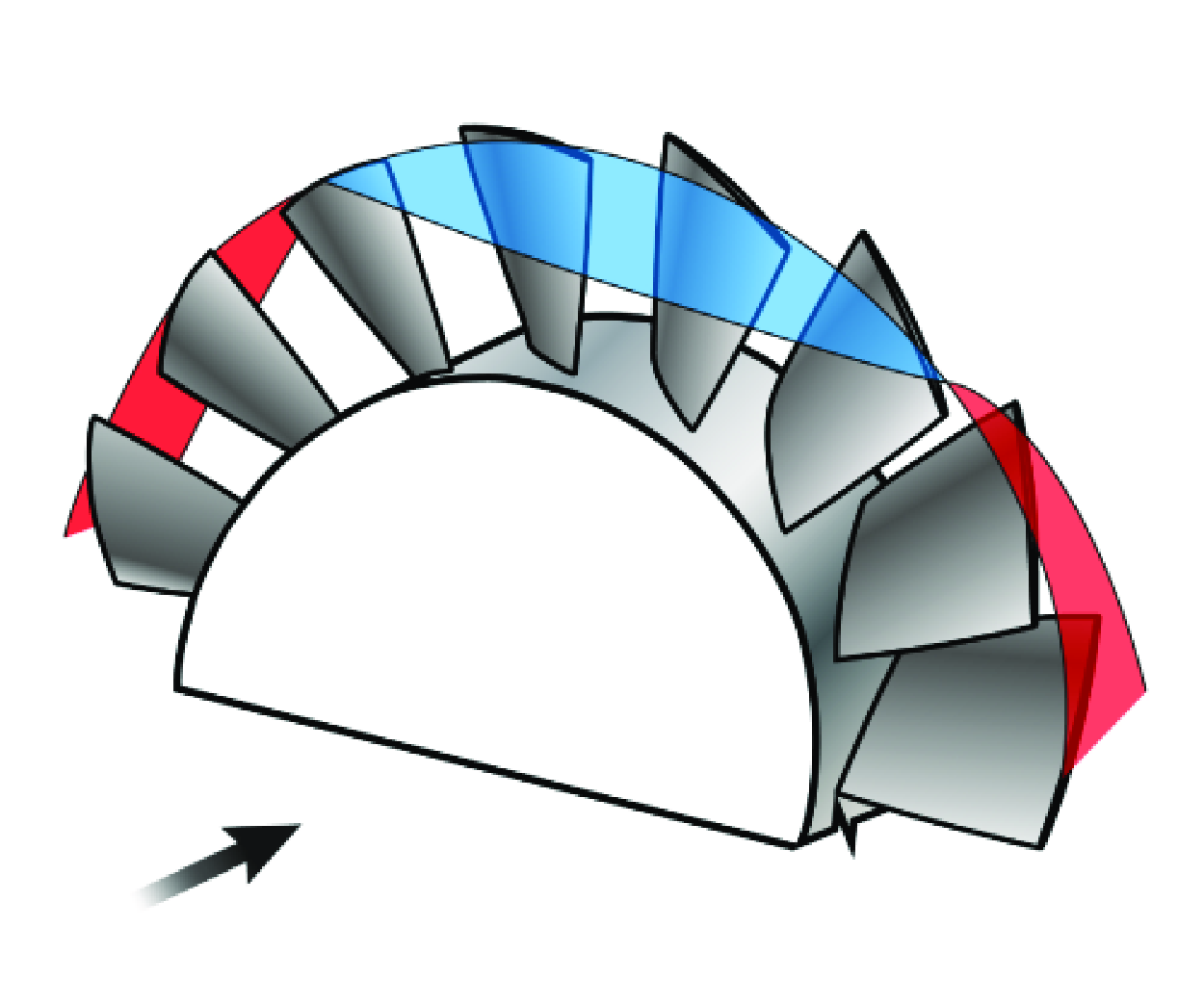
However, the above collected works on rotating resonance modes are all at zero mean flow conditions, which can only be treated as an approximation for slow-flow-speed scenarios (Koch Reference Koch1983). In practical aero-engines, however, the background mean flow Mach number is significantly higher, and the zero-mean-flow assumption is no longer applicable. Therefore, it is of great importance to develop a model capable of predicting the rotating resonance modes in the presence of non-zero background mean flow and to further investigate the corresponding resonance characteristics. Theoretically, Peake’s 2-D model (Woodley & Peake Reference Woodley and Peake1999a ,Reference Woodley and Peake b ) has the potential to estimate the rotating resonances in a 2-D cascade, yet they mainly focused on identifying the inherently unstable resonances between two cascades with zero dissipation and did not pay attention to other resonance modes. In real aero-engines, there exist complex unsteady flows and blade vibrations that may easily act as an external energy source to excite resonances, so a complete solution for all possible resonance modes with and without inherent dissipation is still necessary for practical engineering problems. In addition, three-dimensional (3-D) effects also play an important role in the acoustic prediction of annular cascades with moderately large hub-to-tip ratios. They have a great impact on the cut-off frequencies of the duct modes and thus the estimation of acoustic resonances in annular cascades. A fully 3-D prediction model is therefore necessary for practical cascades, especially for future studies on the effects of tip clearance, where the cascade is inherently non-uniform in the radial direction.

Figure 1. Schematic of a hard-walled annular cascade section and its acoustic scattering.
In this paper, we are devoted to the establishment of a fully 3-D acoustic resonance model for annular cascades in the presence of background mean flow. Such a model is developed in
 $\S$
2 based on our previously established 3-D cascade response (Shen, Wang & Sun Reference Shen, Wang, Sun, Zhang and Sun2022b
). A reduced quasi-3-D cascade of hub-to-tip ratio of 0.99 is first investigated in
$\S$
2 based on our previously established 3-D cascade response (Shen, Wang & Sun Reference Shen, Wang, Sun, Zhang and Sun2022b
). A reduced quasi-3-D cascade of hub-to-tip ratio of 0.99 is first investigated in
 $\S$
3 to reveal general characteristics. Solutions for a fully 3-D cascade are then presented in
$\S$
3 to reveal general characteristics. Solutions for a fully 3-D cascade are then presented in
 $\S$
4, including a comparison with the previous experimental results of Parker & Pryce (Reference Parker and Pryce1974). The effects of the background mean flow are studied in detail, and the mode scattering effect by the cascade shows significant influence on the characteristics of rotating acoustic resonances. Finally, discussions and conclusions are presented in
$\S$
4, including a comparison with the previous experimental results of Parker & Pryce (Reference Parker and Pryce1974). The effects of the background mean flow are studied in detail, and the mode scattering effect by the cascade shows significant influence on the characteristics of rotating acoustic resonances. Finally, discussions and conclusions are presented in
 $\S$
5.
$\S$
5.
2. Formulation
In this paper we consider a stationary annular cascade of
 $V$
straight flat plates of zero thickness and zero stagger, representing radially installed vanes. The cascade is positioned inside an infinite hard-walled duct with a uniform isentropic subsonic axial background mean flow of velocity
$V$
straight flat plates of zero thickness and zero stagger, representing radially installed vanes. The cascade is positioned inside an infinite hard-walled duct with a uniform isentropic subsonic axial background mean flow of velocity
 $U$
. As illustrated in figure 1, the cascade is of uniform hub radius
$U$
. As illustrated in figure 1, the cascade is of uniform hub radius
 $R_h$
, tip radius
$R_h$
, tip radius
 $R_d$
and chord length
$R_d$
and chord length
 $b$
, and the mean density and the speed of sound of the background mean flow are denoted as
$b$
, and the mean density and the speed of sound of the background mean flow are denoted as
 $\rho _0$
and
$\rho _0$
and
 $c_0$
, respectively. All perturbations are assumed to be small and linearisable, and an unsteady Kutta condition is applied to include the viscous effects. The thin-blade assumption is also applied as in previous theoretical models, since the experimental results of Parker (Reference Parker1966) indicate that the thickness of the blades has little effect on the acoustic resonance frequencies of the cascade. Besides, we try to establish a decoupled model to study the properties of the acoustic resonance modes themselves without any specific form of external aerodynamic/aeroelastic source. Accordingly, the thickness noise as well as the trailing-edge self-noise are neglected here. The insignificant quadrupole aeroacoustic source term can also be neglected (Goldstein Reference Goldstein1976, pp. 220–222); therefore, under high-Reynolds-number flow conditions where the viscous stresses on vanes are relatively small, the only dominant aeroacoustic source on cascade vanes is the dipole source caused by the unsteady pressure loading on vanes.
$c_0$
, respectively. All perturbations are assumed to be small and linearisable, and an unsteady Kutta condition is applied to include the viscous effects. The thin-blade assumption is also applied as in previous theoretical models, since the experimental results of Parker (Reference Parker1966) indicate that the thickness of the blades has little effect on the acoustic resonance frequencies of the cascade. Besides, we try to establish a decoupled model to study the properties of the acoustic resonance modes themselves without any specific form of external aerodynamic/aeroelastic source. Accordingly, the thickness noise as well as the trailing-edge self-noise are neglected here. The insignificant quadrupole aeroacoustic source term can also be neglected (Goldstein Reference Goldstein1976, pp. 220–222); therefore, under high-Reynolds-number flow conditions where the viscous stresses on vanes are relatively small, the only dominant aeroacoustic source on cascade vanes is the dipole source caused by the unsteady pressure loading on vanes.
To establish the acoustic transmission and scattering relations of the cascade, we choose two vertical virtual boundaries at the two sides of the cascade to form an isolated section, arbitrarily denoted as Section
 $K$
with an axial length
$K$
with an axial length
 $L_K$
. The upstream and the downstream non-reflective duct sections are denoted as Section
$L_K$
. The upstream and the downstream non-reflective duct sections are denoted as Section
 $K-1$
and Section
$K-1$
and Section
 $K+1$
, respectively. For the zero-sweep straight vanes,
$K+1$
, respectively. For the zero-sweep straight vanes,
 $L_K$
can be taken as
$L_K$
can be taken as
 $L_K=b$
such that the boundaries of Section
$L_K=b$
such that the boundaries of Section
 $K$
coincide with the leading-edge and the trailing-edge planes of the cascade but the section still contains the entire cascade. A cylindrical coordinate system
$K$
coincide with the leading-edge and the trailing-edge planes of the cascade but the section still contains the entire cascade. A cylindrical coordinate system
 $(r,\varphi ,z)$
is applied, and the left boundary is set as the zero point (
$(r,\varphi ,z)$
is applied, and the left boundary is set as the zero point (
 $z=0$
) of the axial coordinate when considering each section. Following classic duct acoustics (Tyler & Sofrin Reference Tyler and Sofrin1962), the downstream-propagating acoustic waves exiting Section
$z=0$
) of the axial coordinate when considering each section. Following classic duct acoustics (Tyler & Sofrin Reference Tyler and Sofrin1962), the downstream-propagating acoustic waves exiting Section
 $K$
at its right boundary can be denoted as
$K$
at its right boundary can be denoted as
 \begin{align} p_{D,K}(r,\varphi ,z,t)=\sum _{m=-\infty }^{+\infty }\sum _{n=0}^{+\infty } D^{K}_{mn}\phi _m(k_{mn}r) \exp \!\big[\mathrm {i} m\varphi +\mathrm {i}\alpha _{1}^{(mn)} (z-L_K) - \mathrm {i}\omega t \big], \end{align}
and, similarly, outgoing acoustic waves propagating upstream from the left boundary of this section can be expressed as
 \begin{align} p_{A,K}(r,\varphi ,z,t)=\sum _{m=-\infty }^{+\infty }\sum _{n=0}^{+\infty } A^{K}_{mn}\phi _m(k_{mn}r) \exp \!\big[\mathrm {i} m\varphi +\mathrm {i}\alpha _{2}^{(mn)} z - \mathrm {i}\omega t \big] , \end{align}
where
 $\omega$
is the angular sound frequency,
$\omega$
is the angular sound frequency,
 $D^{K}_{mn}$
,
$D^{K}_{mn}$
,
 $A^{K}_{mn}$
are the mode amplitude coefficients and
$A^{K}_{mn}$
are the mode amplitude coefficients and
 $\phi _m(k_{mn}r)$
is the normalised radial eigenfunction of the hard-walled annular duct (see Sun & Wang Reference Sun and Wang2021, pp. 95–98) satisfying the orthogonality as
$\phi _m(k_{mn}r)$
is the normalised radial eigenfunction of the hard-walled annular duct (see Sun & Wang Reference Sun and Wang2021, pp. 95–98) satisfying the orthogonality as
 $\int _{R_h}^{R_d}\phi _m(k_{mi}r)\phi _m(k_{mj}r)r\mathrm {d}r=\delta _{ij}$
. Note that a circular cascade can then be easily considered with a simple replacement in the radial eigenfunction
$\int _{R_h}^{R_d}\phi _m(k_{mi}r)\phi _m(k_{mj}r)r\mathrm {d}r=\delta _{ij}$
. Note that a circular cascade can then be easily considered with a simple replacement in the radial eigenfunction
 $\phi _m(k_{mn}r)$
, although this paper focuses on annular cascades. Parameter
$\phi _m(k_{mn}r)$
, although this paper focuses on annular cascades. Parameter
 $k_{mn}$
is the corresponding eigenvalue of circumferential mode number
$k_{mn}$
is the corresponding eigenvalue of circumferential mode number
 $m$
and radial mode number
$m$
and radial mode number
 $n$
, and the acoustic duct modes are denoted as
$n$
, and the acoustic duct modes are denoted as
 $(m,n)$
modes, respectively. The downstream (
$(m,n)$
modes, respectively. The downstream (
 $\alpha _{1}^{(mn)}$
) and upstream (
$\alpha _{1}^{(mn)}$
) and upstream (
 $\alpha _{2}^{(mn)}$
) axial wavenumbers are
$\alpha _{2}^{(mn)}$
) axial wavenumbers are
 \begin{align} \alpha _{1,2}^{(mn)}=\frac {-Mk_0\pm \kappa _{nm}}{\beta ^2},\quad \kappa _{nm} = \big(k_0^2-\beta ^2k_{mn}^2 \big)^{1/2}. \end{align}
Here
 $M=U/c_0$
is the Mach number of the background mean flow,
$M=U/c_0$
is the Mach number of the background mean flow,
 $k_0=\omega /c_0$
is the wavenumber of sound and
$k_0=\omega /c_0$
is the wavenumber of sound and
 $\beta$
is the Prandtl–Glauert transformation factor with
$\beta$
is the Prandtl–Glauert transformation factor with
 $\beta = \sqrt {1-M^2}$
. Note that in search of a resonance characteristic frequency whose real part
$\beta = \sqrt {1-M^2}$
. Note that in search of a resonance characteristic frequency whose real part
 ${\rm Re}(\omega )$
represents the oscillation time period and imaginary part
${\rm Re}(\omega )$
represents the oscillation time period and imaginary part
 ${\rm Im}(\omega )$
indicates the growth rate of the resonance mode amplitude as time increases,
${\rm Im}(\omega )$
indicates the growth rate of the resonance mode amplitude as time increases,
 $\omega$
and in turn the acoustic wavenumber
$\omega$
and in turn the acoustic wavenumber
 $k_0$
are treated as complex numbers, whereas
$k_0$
are treated as complex numbers, whereas
 $\kappa _{nm}$
are chosen directly following the causality condition.
$\kappa _{nm}$
are chosen directly following the causality condition.
The duct is assumed to be hard-walled with constant cross-sections at the virtual boundaries, so there should be no acoustic scattering and the pressure waves propagate continuously across these boundaries. As a result, the acoustic waves entering the left boundary of Section
 $K$
should be equal to the exiting waves of the upstream section (Section
$K$
should be equal to the exiting waves of the upstream section (Section
 $K-1$
) at its right boundary. These incident waves are then expressed as
$K-1$
) at its right boundary. These incident waves are then expressed as
 \begin{align} p_{D,K-1}(r,\varphi ,z,t)=\sum _{m=-\infty }^{+\infty }\sum _{n=0}^{+\infty } D^{K-1}_{mn}\phi _m(k_{mn}r) \exp \!\big[\mathrm {i} m\varphi +\mathrm {i}\alpha _{1}^{(mn)} z - \mathrm {i}\omega t \big] . \end{align}
Similarly, the upstream waves propagating inward Section
 $K$
at its right boundary are the exiting waves of the next section
$K$
at its right boundary are the exiting waves of the next section
 $K+1$
, which are expressed as
$K+1$
, which are expressed as
 \begin{align} p_{A,K+1}(r,\varphi ,z,t)=\sum _{m=-\infty }^{+\infty }\sum _{n=0}^{+\infty } A^{K+1}_{mn}\phi _m(k_{mn}r) \exp \big[\mathrm {i} m\varphi +\mathrm {i}\alpha _{2}^{(mn)}( z-L_K) - \mathrm {i}\omega t \big] . \end{align}
If we further denote the upstream- and downstream-propagating waves scattered from the cascade solid surfaces as
 $p_{s,u}$
and
$p_{s,u}$
and
 $p_{d,u}$
, then the relationship between the acoustic waves at the two virtual boundaries of Section
$p_{d,u}$
, then the relationship between the acoustic waves at the two virtual boundaries of Section
 $K$
can be written as
$K$
can be written as
 \begin{align} p_{A,K}=p_{A,K+1}+p_{s,u}\ \Big |_{z=0} , \quad p_{D,K} = p_{D,K-1}+p_{s,d}\ \Big |_{z=L_K} . \end{align}
Because the mode eigenfunctions are completely orthogonal and there exists no scattering at the section boundaries, the above equations are equivalent to the requirement that for each duct mode
 $(m,n)$
the corresponding mode amplitude coefficients satisfy the equations described in (2.6). Therefore, if the mode amplitudes of the scattered waves
$(m,n)$
the corresponding mode amplitude coefficients satisfy the equations described in (2.6). Therefore, if the mode amplitudes of the scattered waves
 $p_{s,u}$
and
$p_{s,u}$
and
 $p_{s,d}$
can be expressed as a function of the incident waves, the acoustic propagation and scattering relationship of the cascade can be fully described by (2.6) using four sets of amplitude coefficients:
$p_{s,d}$
can be expressed as a function of the incident waves, the acoustic propagation and scattering relationship of the cascade can be fully described by (2.6) using four sets of amplitude coefficients:
 $\{D^{K-1}_{mn}\}$
,
$\{D^{K-1}_{mn}\}$
,
 $\{A^{K}_{mn}\}$
,
$\{A^{K}_{mn}\}$
,
 $\{D^{K}_{mn}\}$
and
$\{D^{K}_{mn}\}$
and
 $\{A^{K+1}_{mn}\}$
.
$\{A^{K+1}_{mn}\}$
.
2.1. Wave scattering
The acoustic scattering of the cascade is described based on our previously established cascade response model (Shen et al. Reference Shen, Wang, Sun, Zhang and Sun2022b ), which is an extension of the 3-D lifting surface method developed by Namba (Reference Namba1972, Reference Namba1977, Reference Namba1987). Using the generalised Lighthill equation by Goldstein (Reference Goldstein1976, pp. 189–192), the scattered pressure field of the thin-blade cascade under high-Reynolds-number background mean flow can be expressed as
 \begin{align} p_s(\boldsymbol {x},t)=\int _{-\infty }^{\infty }\int _{S(\tau )} \frac {\partial G}{r^{\prime}\partial \varphi ^{\prime}} \Delta P_s(\boldsymbol {y})\exp (-\mathrm {i}\omega \tau ) \mathrm {d}S(\boldsymbol {y}) \mathrm {d} \tau , \end{align}
neglecting the insignificant monopole source terms, the volume turbulence quadrupole source terms and the sound radiation caused by the viscous stress dipoles on vane surfaces (Shen et al. Reference Shen, Wang, Sun, Zhang and Sun2022b
). Here and after, the coordinates with superscript
 $^{\prime}$
represent those of the source point and otherwise the observation point. Time
$^{\prime}$
represent those of the source point and otherwise the observation point. Time
 $t$
is the time of observation,
$t$
is the time of observation,
 $\tau$
is the time of source and
$\tau$
is the time of source and
 $\boldsymbol {x,y}$
are respectively the spatial coordinate vectors of the observation point and the source point. Function
$\boldsymbol {x,y}$
are respectively the spatial coordinate vectors of the observation point and the source point. Function
 $G$
is the Green’s function for an infinite hard-walled annular duct with a uniform subsonic axial background mean flow, satisfying Lighthill’s wave equation (Lighthill Reference Lighthill1952) and a boundary condition of zero normal derivative at duct walls. The surface integration
$G$
is the Green’s function for an infinite hard-walled annular duct with a uniform subsonic axial background mean flow, satisfying Lighthill’s wave equation (Lighthill Reference Lighthill1952) and a boundary condition of zero normal derivative at duct walls. The surface integration
 $\int _{S(\tau )}(\cdot ) \mathrm {d}S(\boldsymbol {y})$
takes place over the vanes, and the derivative normal to the surfaces is
$\int _{S(\tau )}(\cdot ) \mathrm {d}S(\boldsymbol {y})$
takes place over the vanes, and the derivative normal to the surfaces is
 ${\partial }/{(r^{\prime}\partial \varphi ^{\prime})}$
for the radially placed vanes with which we studied. The dominant aeroacoustic source during acoustic scattering is the unsteady pressure difference
${\partial }/{(r^{\prime}\partial \varphi ^{\prime})}$
for the radially placed vanes with which we studied. The dominant aeroacoustic source during acoustic scattering is the unsteady pressure difference
 $\Delta P_s$
between the two sides of the vanes.
$\Delta P_s$
between the two sides of the vanes.
In the cylindrical coordinate system illustrated in figure 1, the Green’s function of the hard-walled duct can be expressed as (Sun & Wang Reference Sun and Wang2021, pp. 92–98)
 \begin{align} G(r,\varphi ,z,t\ &\vert \ r^{\prime},\varphi ^{\prime},z^{\prime},\tau ) =\frac {1}{4\pi ^2}\sum _{m=-\infty }^{+\infty }\sum _{n=0}^{+\infty } \frac {\phi _m(k_{mn}r) \phi _m(k_{mn}r^{\prime})}{2\pi } \exp [\mathrm {i}m(\varphi -\varphi ^{\prime})] \nonumber \\[3pt] &\mbox {}\times \int _{-\infty }^{+\infty } \int _{-\infty }^{+\infty } \frac {\exp [\mathrm {i}\alpha (z-z^{\prime})]}{\beta ^2\alpha ^2 + 2Mk_0\alpha -k_0^2+k_{mn}^2} \exp [-\mathrm {i}\omega ^{\prime}(t-\tau )] \,\mathrm {d}\alpha \,\mathrm {d}\omega ^{\prime} .\end{align}
Substituting (2.8) into (2.7) and using the residue theorem to solve for the infinite integral of the axial wavenumber
 $\alpha$
, the scattered sound field can be obtained as an integral of the unknown unsteady pressure loading
$\alpha$
, the scattered sound field can be obtained as an integral of the unknown unsteady pressure loading
 $\Delta P_s$
on the cascade vanes. Considering the circumferential periodicity of the pressure disturbances, the integral can be further simplified to the integral of the unsteady loading distribution
$\Delta P_s$
on the cascade vanes. Considering the circumferential periodicity of the pressure disturbances, the integral can be further simplified to the integral of the unsteady loading distribution
 $\Delta P_s(r^{\prime},z^{\prime})\exp (-\mathrm {i}\omega t)$
on a single reference vane at
$\Delta P_s(r^{\prime},z^{\prime})\exp (-\mathrm {i}\omega t)$
on a single reference vane at
 $\varphi ^{\prime}=0$
(for details, see Shen et al. (Reference Shen, Wang, Sun, Zhang and Sun2022b
)). If we use
$\varphi ^{\prime}=0$
(for details, see Shen et al. (Reference Shen, Wang, Sun, Zhang and Sun2022b
)). If we use
 $\sigma$
to denote the inter-blade phase angle of the incident disturbances as well as the unsteady pressure loading
$\sigma$
to denote the inter-blade phase angle of the incident disturbances as well as the unsteady pressure loading
 $\Delta P_s$
on vanes (as illustrated in figure 1), the scattered pressure fields downstream and upstream of the cascade are obtained as
$\Delta P_s$
on vanes (as illustrated in figure 1), the scattered pressure fields downstream and upstream of the cascade are obtained as
 \begin{align} p_{s,d/u}(\boldsymbol {x},t) & = \exp (-\mathrm {i}\omega t)\sum _{q=-\infty }^{+\infty }\sum _{n=0}^{+\infty }\phi _m(k_{mn}r) \exp (\mathrm {i}m\varphi ) \int _{S_1(\tau )}\frac {mV}{4\pi \kappa _{nm}r^{\prime}} \phi _m(k_{mn}r^{\prime}) \nonumber \\[3pt] & \quad \times \Delta P_s(r^{\prime},z^{\prime}) \left \{ \mathrm {H}(\pm z \mp z^{\prime})\exp \big[\mathrm {i}\alpha_{1,2}^{(m,n)}(z-z^{\prime})\big] \right \} \mathrm {d}S(\boldsymbol {y}) ,\quad m=\frac {V\sigma }{2\pi }-qV. \end{align}
Here
 $\mathrm {H}(\cdot )$
denotes the Heaviside function. Besides, the surface integral domain also reduces to that of one single vane
$\mathrm {H}(\cdot )$
denotes the Heaviside function. Besides, the surface integral domain also reduces to that of one single vane
 $S_1(\tau )$
located at
$S_1(\tau )$
located at
 $\varphi ^{\prime}=0$
.
$\varphi ^{\prime}=0$
.
Referring to the linearised inviscid momentum equation, the circumferential induced velocity of the scattered field is obtained as
 \begin{align} v_\varphi (\boldsymbol {x},t) = & -\frac {V\mathrm {e}^{-\mathrm {i}\omega t}}{2\pi \rho _0 U}\sum _{q=-\infty }^{+\infty }\sum _{n=0}^{+\infty }\frac {m}{r}\phi _m(k_{mn}r)\exp (\mathrm {i}m\varphi ) \int _{S_1(\tau )}\frac {m}{r^{\prime}} \phi _m(k_{mn}r^{\prime}) \Delta P_s(r^{\prime},z^{\prime}) \nonumber \\[3pt] &\mbox {}\times \left \{\mathrm {H}(z-z^{\prime})[Q_1 +Q_3] + \mathrm {H}(z^{\prime}-z) Q_2 \right \} \mathrm {d}S(\boldsymbol {y}) ,\quad m=\frac {V\sigma }{2\pi }-qV, \end{align}
where the coefficients are
 \begin{align} Q_{1,2} = \frac {M\beta ^2\exp\!\big [\mathrm {i}\alpha _{1,2}^{(mn)}(z-z^{\prime}) \big]}{2\kappa _{nm}(\pm M\kappa _{nm}-k_0)}, \quad Q_3 = \frac {M^2 \exp [{\rm i}\alpha _3(z-z^{\prime})]}{k_0^2+M^2 k_{mn}^2}, \end{align}
and the axial wavenumber of shed vortical waves is
 $\alpha _3=\omega /U=k_0/M$
. The integral terms with
$\alpha _3=\omega /U=k_0/M$
. The integral terms with
 $Q_{1,2}$
correspond to the velocity induced by the downstream- and upstream-propagating acoustic waves, and the integral term with
$Q_{1,2}$
correspond to the velocity induced by the downstream- and upstream-propagating acoustic waves, and the integral term with
 $Q_3$
corresponds to the velocity induced by the shed vortical waves. In addition, the circumferential particle velocity of any propagating acoustic waves with mode amplitude coefficient
$Q_3$
corresponds to the velocity induced by the shed vortical waves. In addition, the circumferential particle velocity of any propagating acoustic waves with mode amplitude coefficient
 $A_{mn}$
can also be derived as
$A_{mn}$
can also be derived as
 \begin{align} u_\varphi =-\frac {1}{\rho _0 U }\frac {m}{\big(\alpha _{1,2}^{(mn)}-\alpha _3 \big)r} A_{mn}\phi _m(k_{mn}r) \exp \!\big[\mathrm {i} m\varphi +\mathrm {i}\alpha _{1,2}^{(mn)} z - \mathrm {i}\omega t \big] . \end{align}
On the vane surfaces, the upwash velocities should satisfy the zero normal velocity boundary condition for a solid cascade:
 \begin{align} v_\varphi = -u_\varphi . \end{align}
Substituting (2.10) and (2.12) into (2.13) and dropping the time harmonic factor
 $\exp (-\mathrm {i}\omega t)$
, we can establish an integral equation about the unknown dipole source distribution
$\exp (-\mathrm {i}\omega t)$
, we can establish an integral equation about the unknown dipole source distribution
 $\Delta P_s(r^{\prime},z^{\prime})$
with any given incident acoustic wave, including the previously described incident waves (2.4) and (2.5). Then we can numerically solve the integral equation to obtain
$\Delta P_s(r^{\prime},z^{\prime})$
with any given incident acoustic wave, including the previously described incident waves (2.4) and (2.5). Then we can numerically solve the integral equation to obtain
 $\Delta P_s(r^{\prime},z^{\prime})$
and derive the mode amplitude coefficients of the scattered sound field
$\Delta P_s(r^{\prime},z^{\prime})$
and derive the mode amplitude coefficients of the scattered sound field
 $p_{s,u}$
and
$p_{s,u}$
and
 $p_{s,d}$
using (2.9).
$p_{s,d}$
using (2.9).
2.2. Solution of characteristic frequencies
A collocation method is applied to solve the integral equation (2.13) established above. Within the linear range where there is no flow separation, the unsteady Kutta condition of subsonic background mean flow can be applied in a similar way to the steady case (Crighton Reference Crighton1985). Following the hybrid method proposed by Namba (Reference Namba1987), the unsteady pressure loading
 $\Delta P_s(r^{\prime},z^{\prime})$
can be expanded as
$\Delta P_s(r^{\prime},z^{\prime})$
can be expanded as
 \begin{align} \Delta P_s(r^{\prime},z^{\prime}) \big |_{r^{\prime}=R_h + (2j^{\prime}-1)(R_d-R_h)/(2J)}=\left [ B_{1j^{\prime}} \cot \left (\frac {\xi ^{\prime}}{2}\right ) + \sum _{i^{\prime}=2}^{I}B_{i^{\prime}j^{\prime}}\sin \big ((i^{\prime}-1)\xi ^{\prime}\big ) \right ] , \end{align}
with
 $I$
axial terms and
$I$
axial terms and
 $J$
radial terms, and the distribution of
$J$
radial terms, and the distribution of
 $\Delta P_s(r^{\prime},z^{\prime})$
can therefore be represented by a series of expansion coefficients
$\Delta P_s(r^{\prime},z^{\prime})$
can therefore be represented by a series of expansion coefficients
 $\{B_{i^{\prime}j^{\prime}}\}$
. In the radial direction,
$\{B_{i^{\prime}j^{\prime}}\}$
. In the radial direction,
 $\Delta P_s(r^{\prime},z^{\prime})$
is discretised and the subscript
$\Delta P_s(r^{\prime},z^{\prime})$
is discretised and the subscript
 $j^{\prime}$
denotes the radial positions of each slice. This could provide convenience to consider swept vanes in future studies. In the axial direction, the distribution of
$j^{\prime}$
denotes the radial positions of each slice. This could provide convenience to consider swept vanes in future studies. In the axial direction, the distribution of
 $\Delta P_s(r^{\prime},z^{\prime})$
is expanded as cotangent and sine functions. In addition, Glauert’s transformation is applied to the axial coordinates for both the source position
$\Delta P_s(r^{\prime},z^{\prime})$
is expanded as cotangent and sine functions. In addition, Glauert’s transformation is applied to the axial coordinates for both the source position
 $z^{\prime}$
and the observation location
$z^{\prime}$
and the observation location
 $z$
as
$z$
as
 \begin{align} z^{\prime}=\frac {b}{2}(1-\cos \xi ^{\prime}),\quad z=\frac {b}{2}(1-\cos \xi ),\quad z^{\prime},z\in [0,b],\ \xi ^{\prime},\xi \in [0,\pi ]. \end{align}
The unsteady Kutta condition is inherently applied here (Rienstra Reference Rienstra1992). The convergence of numerical solution is checked a posteriori. If the solution of the series (2.14) converges, it should converge to the Kutta solution, i.e. the physical solution which satisfies the experimental results with practical viscosity effects (Crighton Reference Crighton1985). After dropping the time harmonic factor
 $\exp (-\mathrm {i}\omega t)$
, the integral equation (2.13) is then enforced at
$\exp (-\mathrm {i}\omega t)$
, the integral equation (2.13) is then enforced at
 $J \times I$
evenly spaced control points at observation positions
$J \times I$
evenly spaced control points at observation positions
 $(r_j,\xi _i)$
, where
$(r_j,\xi _i)$
, where
 \begin{align} r_{j}=\frac {(2j-1)(R_d-R_h)}{J}, \quad \xi _i=\frac {(2i-1)\pi }{2I}, \quad j=1,\dots ,J, \quad i=1,\dots ,I. \end{align}
The left-hand side of the equation is numerically integrated using the trapezoidal rule at axial source points similar to that in Whitehead (Reference Whitehead1962), with the unsteady loading source expansion (2.14) substituted in. Therefore, the integral equation (2.13) is finally discretised into a system of linear equations written in a matrix equation form as
 \begin{align} \unicode{x1D648}_{ij,i^{\prime}j^{\prime}}\boldsymbol {B}_{i^{\prime}j^{\prime}}=-\boldsymbol {u}_{\varphi ,ij} \Big |_{(r,\xi )=(r_j,\xi _i)} , \end{align}
similar to the process in Shen et al. (Reference Shen, Wang, Sun, Zhang and Sun2022b
). Here the square matrix
 $\unicode{x1D648}$
correlates the dipole expansion coefficients
$\unicode{x1D648}$
correlates the dipole expansion coefficients
 ${\boldsymbol{B}}_{i^{\prime}j^{\prime}}$
to the induced velocity
${\boldsymbol{B}}_{i^{\prime}j^{\prime}}$
to the induced velocity
 ${\boldsymbol{u}}_{\varphi ,ij}$
at the control points on vanes.
${\boldsymbol{u}}_{\varphi ,ij}$
at the control points on vanes.
Now we can establish the scattering equations between the incident and out-going amplitude coefficients
 $\{D^{K-1}_{mn}\}$
,
$\{D^{K-1}_{mn}\}$
,
 $\{A^{K}_{mn}\}$
,
$\{A^{K}_{mn}\}$
,
 $\{D^{K}_{mn}\}$
and
$\{D^{K}_{mn}\}$
and
 $\{A^{K+1}_{mn}\}$
. Firstly, a main circumferential mode number
$\{A^{K+1}_{mn}\}$
. Firstly, a main circumferential mode number
 $m_0$
is chosen, corresponding to an inter-blade phase angle
$m_0$
is chosen, corresponding to an inter-blade phase angle
 $\sigma =2\pi m_0 / V$
. The radial modes are then truncated at
$\sigma =2\pi m_0 / V$
. The radial modes are then truncated at
 $n=N$
and the circumferential modes
$n=N$
and the circumferential modes
 $m=m_0+qV$
are truncated at
$m=m_0+qV$
are truncated at
 $m=m_0\pm MV$
, such that each amplitude coefficient vector
$m=m_0\pm MV$
, such that each amplitude coefficient vector
 $\boldsymbol {D/A}^{\sim }_{mn}$
has a total of
$\boldsymbol {D/A}^{\sim }_{mn}$
has a total of
 $(2M+1)\times N$
terms. Accordingly, the upwash velocity vector
$(2M+1)\times N$
terms. Accordingly, the upwash velocity vector
 $\boldsymbol {u}_{\varphi ,ij}$
induced by the incident coefficients
$\boldsymbol {u}_{\varphi ,ij}$
induced by the incident coefficients
 $\{D^{K-1}_{mn}\}$
and
$\{D^{K-1}_{mn}\}$
and
 $\{A^{K+1}_{mn}\}$
can be calculated as
$\{A^{K+1}_{mn}\}$
can be calculated as
 $\boldsymbol {u}_{\varphi ,ij}=\unicode{x1D64F}^{D}_{ij,mn}\boldsymbol {D}^{K-1}_{mn}(\mathrm {or}\ \unicode{x1D64F}^{A}_{ij,mn}\boldsymbol {A}^{K+1}_{mn})$
using matrices
$\boldsymbol {u}_{\varphi ,ij}=\unicode{x1D64F}^{D}_{ij,mn}\boldsymbol {D}^{K-1}_{mn}(\mathrm {or}\ \unicode{x1D64F}^{A}_{ij,mn}\boldsymbol {A}^{K+1}_{mn})$
using matrices
 \begin{align} \unicode{x1D64F}^{D(A)}_{ij,mn}=\frac {1}{\rho _0 U}\frac {m}{r_j}\frac {\phi _m(k_{mn}r_j) \exp\!\big[\mathrm {i} \alpha _{1(2)}^{(mn)} (z_i - 0.5 L_K\pm 0.5L_K) \big]}{\alpha _{1(2)}^{(mn)}-\omega /U} , \end{align}
by referring to (2.12). The acoustic mode amplitude coefficients of the scattered field can be calculated by matrix multiplication
 $\unicode{x1D64E}^{D(A)}_{mn,i^{\prime}j^{\prime}} \boldsymbol {B}_{i^{\prime}j^{\prime}}$
, corresponding to the numerical integration of (2.9) with the unsteady loading expansion (2.14). Therefore, the scattering relations restricted by (2.6) can be finally rearranged and rewritten as a matrix equation with the incident wave amplitudes on the right-hand side:
$\unicode{x1D64E}^{D(A)}_{mn,i^{\prime}j^{\prime}} \boldsymbol {B}_{i^{\prime}j^{\prime}}$
, corresponding to the numerical integration of (2.9) with the unsteady loading expansion (2.14). Therefore, the scattering relations restricted by (2.6) can be finally rearranged and rewritten as a matrix equation with the incident wave amplitudes on the right-hand side:
 \begin{align} \unicode{x1D653}(\omega )\left [ \begin{array}{c} \boldsymbol {A}^{K}_{mn} \\[3pt] \displaystyle \boldsymbol {D}^{K}_{mn} \end{array} \right ] =\left [\begin{array}{c@{\quad}c} \unicode{x1D668}\unicode{x1D668}_{LL}\ &\ \unicode{x1D668}\unicode{x1D668}_{RL} \\[3pt] \displaystyle \unicode{x1D668}\unicode{x1D668}_{LR}\ &\ \unicode{x1D668}\unicode{x1D668}_{RR} \end{array} \right ] ^{-1} \left [ \begin{array}{c} \boldsymbol {A}^{K}_{mn} \\[3pt] \displaystyle \boldsymbol {D}^{K}_{mn} \end{array} \right ] =\left [ \begin{array}{c} \boldsymbol {D}^{K-1}_{\mu \nu } \\[3pt] \displaystyle \boldsymbol {A}^{K+1}_{\mu \nu } \end{array} \right ] , \end{align}
where
 \begin{eqnarray} &\unicode{x1D668}\unicode{x1D668}_{LL}= \unicode{x1D64E}_{mn,i^{\prime}j^{\prime}}^{A} \unicode{x1D648}_{ij,i^{\prime}j^{\prime}}^{-1} \unicode{x1D64F}^{D}_{ij,\mu \nu } , \end{eqnarray}
 \begin{eqnarray} &\unicode{x1D668}\unicode{x1D668}_{RL}= \unicode{x1D64E}_{mn,i^{\prime}j^{\prime}}^{A} \unicode{x1D648}_{ij,i^{\prime}j^{\prime}}^{-1} \unicode{x1D64F}^{A}_{ij,\mu \nu } + \left [\delta _{m \mu }\delta _{n \nu }\exp\!\big(-\mathrm {i}\alpha _{2}^{(\mu \nu )} L_K \big)\right ]_{mn,\mu \nu } , \end{eqnarray}
 \begin{eqnarray} &\unicode{x1D668}\unicode{x1D668}_{LR}= \unicode{x1D64E}_{mn,i^{\prime}j^{\prime}}^{D} \unicode{x1D648}_{ij,i^{\prime}j^{\prime}}^{-1} \unicode{x1D64F}^{D}_{ij,\mu \nu } + \left [\delta _{m \mu }\delta _{n \nu }\exp \!\big(\mathrm {i}\alpha _{1}^{(\mu \nu )} L_K \big)\right ]_{mn,\mu \nu } , \end{eqnarray}
 \begin{eqnarray} &\unicode{x1D668}\unicode{x1D668}_{RR}= \unicode{x1D64E}_{mn,i^{\prime}j^{\prime}}^{D} \unicode{x1D648}_{ij,i^{\prime}j^{\prime}}^{-1} \unicode{x1D64F}^{A}_{ij,\mu \nu } . \end{eqnarray}
To solve for the acoustic resonances of the isolated cascade, we assume zero incident waves and zero reflections at the upstream and downstream boundaries. The acoustic resonance states then correspond to the non-zero solutions of the scattering equation (2.19) with zero right-hand side, i.e.
 $\boldsymbol {D}^{K-1}_{\mu \nu } =\boldsymbol {A}^{K+1}_{\mu \nu }=\boldsymbol {0}$
. The resonance characteristic frequencies can thus be calculated by the existence condition of such non-zero solutions,
$\boldsymbol {D}^{K-1}_{\mu \nu } =\boldsymbol {A}^{K+1}_{\mu \nu }=\boldsymbol {0}$
. The resonance characteristic frequencies can thus be calculated by the existence condition of such non-zero solutions,
 $\det [\unicode{x1D653}(\omega )]=0$
, which is equivalent to the requirement that matrix
$\det [\unicode{x1D653}(\omega )]=0$
, which is equivalent to the requirement that matrix
 $\unicode{x1D653}(\omega )$
is singular at the resonance frequency.
$\unicode{x1D653}(\omega )$
is singular at the resonance frequency.
Note that the interactions between the vortical waves shed from the trailing edges of the cascade and other downstream structures in the duct are temporarily ignored, such that they induce no acoustic waves propagating backward to Section
 $K$
from the downstream section. As a result, the vortical waves shed by the thin-blade cascade are not included in the scattering relation (2.19) for simplicity, but they can be easily added to the equations similar to that in Hanson (Reference Hanson1997) or Zhang et al. (Reference Zhang, Wang, Du and Sun2019) if needed. More complex geometries can be considered in the future by further extending the present model to include more sections and using similar non-scattering boundary conditions to connect them together and form a larger matrix
$K$
from the downstream section. As a result, the vortical waves shed by the thin-blade cascade are not included in the scattering relation (2.19) for simplicity, but they can be easily added to the equations similar to that in Hanson (Reference Hanson1997) or Zhang et al. (Reference Zhang, Wang, Du and Sun2019) if needed. More complex geometries can be considered in the future by further extending the present model to include more sections and using similar non-scattering boundary conditions to connect them together and form a larger matrix
 $\unicode{x1D653}(\omega )$
for the solution of characteristic frequencies. In this paper, however, we focus on the most general cascade resonance characteristics by studying one single isolated stator section.
$\unicode{x1D653}(\omega )$
for the solution of characteristic frequencies. In this paper, however, we focus on the most general cascade resonance characteristics by studying one single isolated stator section.
The effect of swirl flow is also temporarily not included, due to the lack of an appropriate analytic Green’s function for 3-D swirled annular flow. Only zero-stagger stator cascades can be strictly considered using the present model. But as shown in Koch (Reference Koch1983), the effect of swirl (or stagger angle) on resonance frequencies is significant when the stagger angle exceeds
 $30^\circ$
, but is much less profound otherwise. Therefore, at the inlet/outlet stages of a fan/compressor where there only exists mild swirl, the above model should be able to provide a good prediction for the acoustic resonances in practical cascades.
$30^\circ$
, but is much less profound otherwise. Therefore, at the inlet/outlet stages of a fan/compressor where there only exists mild swirl, the above model should be able to provide a good prediction for the acoustic resonances in practical cascades.
The commonly used singular value decomposition (SVD) method (as in Woodley & Peake Reference Woodley and Peake1999a
) is applied to search for the complex characteristic frequencies at which the scattering matrix
 $\unicode{x1D653}(\omega )$
is singular. The matrix
$\unicode{x1D653}(\omega )$
is singular. The matrix
 $\unicode{x1D653}(\omega )$
for a given frequency
$\unicode{x1D653}(\omega )$
for a given frequency
 $\omega$
is factorised as a product of two orthogonal matrices and a real diagonal matrix
$\omega$
is factorised as a product of two orthogonal matrices and a real diagonal matrix
 $\unicode{x1D63F}$
using the SVD method, and the condition number of the original matrix can then be calculated by the ratio between the largest and smallest elements of the diagonal matrix
$\unicode{x1D63F}$
using the SVD method, and the condition number of the original matrix can then be calculated by the ratio between the largest and smallest elements of the diagonal matrix
 $\unicode{x1D63F}$
. Finally, a self-adaptive local mesh refinement method is applied to locate the maximum points for the condition number of matrix
$\unicode{x1D63F}$
. Finally, a self-adaptive local mesh refinement method is applied to locate the maximum points for the condition number of matrix
 $\unicode{x1D653}(\omega )$
in the complex frequency plane, which should be the resonance frequencies corresponding to different non-zero solutions (different acoustic resonance modes). Similar to the previous 2-D model by Woodley & Peake (Reference Woodley and Peake1999a
), the resonance results converge rapidly with truncation number
$\unicode{x1D653}(\omega )$
in the complex frequency plane, which should be the resonance frequencies corresponding to different non-zero solutions (different acoustic resonance modes). Similar to the previous 2-D model by Woodley & Peake (Reference Woodley and Peake1999a
), the resonance results converge rapidly with truncation number
 $M$
and
$M$
and
 $N$
such that just a few additional cut-off modes are needed in the calculations.
$N$
such that just a few additional cut-off modes are needed in the calculations.
3. Resonances with a reduced quasi-3-D cascade
We first simplify our model to a quasi-3-D case with annular cascades of hub-to-tip ratio 0.99, in order to reveal general characteristics about the rotating resonance modes under non-zero background mean flow. In this case only the first radial mode
 $n=0$
is considered. Comparison is first made with the ideal 2-D results for the stationary Parker modes predicted by the Wiener–Hopf method (Koch Reference Koch1983), as shown in figure 2. There is no stagger for both stator cascades, and the geometry and flow parameters for the quasi-3-D annular cascade are chosen to be
$n=0$
is considered. Comparison is first made with the ideal 2-D results for the stationary Parker modes predicted by the Wiener–Hopf method (Koch Reference Koch1983), as shown in figure 2. There is no stagger for both stator cascades, and the geometry and flow parameters for the quasi-3-D annular cascade are chosen to be
 \begin{align} V=48,\quad R_h=0.99\ \mathrm {m}, \quad R_d=1.0\ \mathrm {m}, \quad c_0=340.0\ \mathrm {m\,s^{-1}},\quad \rho _0 = 1.225\ \mathrm {kg\,m^{-3}}. \end{align}
Correspondingly, the chord-to-pitch ratio is varied by changing the chord length
 $b$
in the present model. Our predictions for both the real parts and the imaginary parts of the resonance frequencies
$b$
in the present model. Our predictions for both the real parts and the imaginary parts of the resonance frequencies
 $\omega _k$
of Parker’s
$\omega _k$
of Parker’s
 $\beta$
mode match well with the 2-D results of Koch.
$\beta$
mode match well with the 2-D results of Koch.

Figure 2. Comparison between (a) the real parts and (b) the imaginary parts of the resonance frequencies predicted by the present model and results of the 2-D model (figure 5 in Koch (Reference Koch1983)), where the reduced frequency is defined as
 $f^*=(\omega _k d_0)/(2\pi c_0)$
, in which
$f^*=(\omega _k d_0)/(2\pi c_0)$
, in which
 $d_0$
is the cascade pitch and equal to
$d_0$
is the cascade pitch and equal to
 $\pi (R_d+R_h)/V$
in the present model. The imaginary part is unified using the
$\pi (R_d+R_h)/V$
in the present model. The imaginary part is unified using the
 $\mathrm {e}^{-\mathrm {i}\omega t}$
time harmonic notation.
$\mathrm {e}^{-\mathrm {i}\omega t}$
time harmonic notation.

Figure 3. Resonance frequencies of rotating modes in a cascade of solidity
 $2.0$
, with varying circumferential mode number
$2.0$
, with varying circumferential mode number
 $m_0$
and different background mean flow Mach number
$m_0$
and different background mean flow Mach number
 $M=U/c_0$
. The reduced frequency is defined as
$M=U/c_0$
. The reduced frequency is defined as
 $f^*=(\omega _k d_0)/(2\pi c_0)$
, with
$f^*=(\omega _k d_0)/(2\pi c_0)$
, with
 $d_0 = \pi (R_d+R_h)/V$
. Frequency (a) real parts determine the fluctuation time periods and (b) imaginary parts indicate the growth rate of the resonance mode. At
$d_0 = \pi (R_d+R_h)/V$
. Frequency (a) real parts determine the fluctuation time periods and (b) imaginary parts indicate the growth rate of the resonance mode. At
 $m_0=V/2=24$
and
$m_0=V/2=24$
and
 $m_0=V=48$
the resonance modes reduce to the typical Parker’s stationary modes.
$m_0=V=48$
the resonance modes reduce to the typical Parker’s stationary modes.
3.1. General characteristics for rotating resonance frequencies
We then calculate for the resonance frequencies
 $\omega _k$
with continuously varying main mode order
$\omega _k$
with continuously varying main mode order
 $m_0$
(which corresponds to different inter-blade phase angle
$m_0$
(which corresponds to different inter-blade phase angle
 $\sigma$
), including both the rotational acoustic resonances and the stationary Parker modes. The same notations as in Koch (Reference Koch1983) are adopted in this section for the stationary Parker modes, where higher-order modes are denoted as
$\sigma$
), including both the rotational acoustic resonances and the stationary Parker modes. The same notations as in Koch (Reference Koch1983) are adopted in this section for the stationary Parker modes, where higher-order modes are denoted as
 $(q,0)$
(
$(q,0)$
(
 $|\sigma |=\pi$
) or
$|\sigma |=\pi$
) or
 $(q,1)$
(
$(q,1)$
(
 $|\sigma |=2\pi$
) modes, with
$|\sigma |=2\pi$
) modes, with
 $q$
denoting the axial order of the resonance. Note that an unstaggered stator cascade is studied such that the acoustic modes of positive and negative circumferential mode number
$q$
denoting the axial order of the resonance. Note that an unstaggered stator cascade is studied such that the acoustic modes of positive and negative circumferential mode number
 $m$
are symmetric to each other. Therefore, we only present results with positive
$m$
are symmetric to each other. Therefore, we only present results with positive
 $m_0$
, which are the same as for the
$m_0$
, which are the same as for the
 $-m_0$
resonance modes. Results with
$-m_0$
resonance modes. Results with
 $m_0$
up to
$m_0$
up to
 $m_0=V=48$
under different background flow speed are shown in figure 3, using the same geometry set-up as above and a fixed chord-to-pitch ratio (solidity) of 2.0. The resonance frequencies
$m_0=V=48$
under different background flow speed are shown in figure 3, using the same geometry set-up as above and a fixed chord-to-pitch ratio (solidity) of 2.0. The resonance frequencies
 $\omega _k$
are normalised following the same approach as in Koch (Reference Koch1983) and the reduced frequency is defined as
$\omega _k$
are normalised following the same approach as in Koch (Reference Koch1983) and the reduced frequency is defined as
 $f^*=(\omega _k d_0)/(2\pi c_0)$
, where the pitch at mid-radius
$f^*=(\omega _k d_0)/(2\pi c_0)$
, where the pitch at mid-radius
 $R_m=(R_d+R_h)/2$
is
$R_m=(R_d+R_h)/2$
is
 $d_0=\pi (R_d+R_h)/V$
.
$d_0=\pi (R_d+R_h)/V$
.
The real parts of resonance frequencies
 $\omega _k$
show rather organised distributions over certain branches beginning at
$\omega _k$
show rather organised distributions over certain branches beginning at
 $m_0=V/2=24$
or
$m_0=V/2=24$
or
 $m_0=V=48$
. At all branches, the oscillation frequency
$m_0=V=48$
. At all branches, the oscillation frequency
 ${\rm Re}(\omega _k)$
initiates from that of the classic stationary Parker modes and monotonically decreases with
${\rm Re}(\omega _k)$
initiates from that of the classic stationary Parker modes and monotonically decreases with
 $m_0$
, eventually approaching the cut-off frequency
$m_0$
, eventually approaching the cut-off frequency
 $\varOmega$
(Tyler & Sofrin Reference Tyler and Sofrin1962). Therefore, we may define each resonance branch as ‘
$\varOmega$
(Tyler & Sofrin Reference Tyler and Sofrin1962). Therefore, we may define each resonance branch as ‘
 $\mathrm {x}$
-type resonances’, named after the stationary modes they start from, as shown in the legend of figure 3.
$\mathrm {x}$
-type resonances’, named after the stationary modes they start from, as shown in the legend of figure 3.
Similar to the stationary mode results in figure 2, as the background mean flow Mach number
 $M$
increases, the cut-off frequencies of the duct modes will reduce, and the real parts of all resonance characteristic frequencies at different
$M$
increases, the cut-off frequencies of the duct modes will reduce, and the real parts of all resonance characteristic frequencies at different
 $m_0$
decrease. The negative imaginary parts of the characteristic frequencies, however, show different trends between the modes with
$m_0$
decrease. The negative imaginary parts of the characteristic frequencies, however, show different trends between the modes with
 $0\lt m_0\le V/2$
and
$0\lt m_0\le V/2$
and
 $V/2\lt m_0\le V$
. For modes with
$V/2\lt m_0\le V$
. For modes with
 $0\lt m_0\le V/2$
,
$0\lt m_0\le V/2$
,
 ${\rm Im}(\omega _k)$
decreases as
${\rm Im}(\omega _k)$
decreases as
 $M$
increases. For modes with
$M$
increases. For modes with
 $V/2\lt m_0\le V$
,
$V/2\lt m_0\le V$
,
 ${\rm Im}(\omega _k)$
does not necessarily decrease with higher background flow speed. The increase in the absolute value of the growth rate
${\rm Im}(\omega _k)$
does not necessarily decrease with higher background flow speed. The increase in the absolute value of the growth rate
 $|{\rm Im}(\omega _k)|$
indicates that more energy dissipation occurs for the resonance modes. The detailed mechanisms behind the variations in the inherent dissipation are discussed later.
$|{\rm Im}(\omega _k)|$
indicates that more energy dissipation occurs for the resonance modes. The detailed mechanisms behind the variations in the inherent dissipation are discussed later.
As the background flow speed increases, the number of the rotating resonance modes of each resonance branch also augments, and the left bound of each branch approaches an even lower circumferential mode order
 $m_0$
(as, for example, indicated by the black arrow at the top-right corner in figure 3). Note also that at each resonance branch, the difference between two neighbouring
$m_0$
(as, for example, indicated by the black arrow at the top-right corner in figure 3). Note also that at each resonance branch, the difference between two neighbouring
 ${\rm Re}(\omega _k)$
will gradually reduce as
${\rm Re}(\omega _k)$
will gradually reduce as
 $m_0$
increases. But if we just look at a few modes with continuously varying circumferential mode number
$m_0$
increases. But if we just look at a few modes with continuously varying circumferential mode number
 $m_0$
, the corresponding oscillation frequencies
$m_0$
, the corresponding oscillation frequencies
 ${\rm Re}(\omega _k)$
may show a nearly constant interval with a slight decrease as
${\rm Re}(\omega _k)$
may show a nearly constant interval with a slight decrease as
 $m_0$
increases. This characteristic is in agreement with the previous experimental results for practical axial compressor cascades (Parker Reference Parker1968; Camp Reference Camp1999; Holzinger et al. Reference Holzinger, Wartzek, Schiffer, Leichtfuss and Nestle2015).
$m_0$
increases. This characteristic is in agreement with the previous experimental results for practical axial compressor cascades (Parker Reference Parker1968; Camp Reference Camp1999; Holzinger et al. Reference Holzinger, Wartzek, Schiffer, Leichtfuss and Nestle2015).
3.2. Mode amplitude distributions of acoustic resonances
Physically, each characteristic frequency
 $\omega _k$
should correspond to a resonance state with a specific pressure distribution pattern; hence we may assume that at each
$\omega _k$
should correspond to a resonance state with a specific pressure distribution pattern; hence we may assume that at each
 $\omega _k$
the coefficient matrix
$\omega _k$
the coefficient matrix
 $\unicode{x1D653}(\omega _k)$
of order
$\unicode{x1D653}(\omega _k)$
of order
 $2(2M+1)N$
has a rank of
$2(2M+1)N$
has a rank of
 $2(2M+1)N-1$
. The basic solution of the outgoing wave mode amplitudes at each resonance state can be obtained with the procedure as follows. The upstream amplitude coefficient of the first radial mode at main circumferential mode order
$2(2M+1)N-1$
. The basic solution of the outgoing wave mode amplitudes at each resonance state can be obtained with the procedure as follows. The upstream amplitude coefficient of the first radial mode at main circumferential mode order
 $m_0$
is set as 1, i.e.
$m_0$
is set as 1, i.e.
 $A^K_{m_0 0}=1$
. The other mode amplitude coefficients are solved using the least-squares method with a pseudo-inverse matrix. To do so, equation (2.19) with zero right-hand side is rearranged into an overdetermined equation system, where the opposite of the column vector in
$A^K_{m_0 0}=1$
. The other mode amplitude coefficients are solved using the least-squares method with a pseudo-inverse matrix. To do so, equation (2.19) with zero right-hand side is rearranged into an overdetermined equation system, where the opposite of the column vector in
 $\unicode{x1D653}(\omega _k)$
relating to coefficient
$\unicode{x1D653}(\omega _k)$
relating to coefficient
 $A^K_{m_0 0}$
is moved to the right-hand side. As a result, we can directly compare the relative strength between the basic duct mode
$A^K_{m_0 0}$
is moved to the right-hand side. As a result, we can directly compare the relative strength between the basic duct mode
 $m_0$
and its inevitable higher-circumferential-order scattered modes, and further reveal the mode scattering effect by the cascade at resonance states. These are rarely seen in previous theoretical investigations. This procedure also helps to further classify the resonance states calculated with the SVD method by identifying the dominant acoustic mode with the largest amplitude, because due to aliasing, one inter-blade phase angle
$m_0$
and its inevitable higher-circumferential-order scattered modes, and further reveal the mode scattering effect by the cascade at resonance states. These are rarely seen in previous theoretical investigations. This procedure also helps to further classify the resonance states calculated with the SVD method by identifying the dominant acoustic mode with the largest amplitude, because due to aliasing, one inter-blade phase angle
 $\sigma$
can correspond to multiple solutions of characteristic frequency
$\sigma$
can correspond to multiple solutions of characteristic frequency
 $\omega _k$
with different dominant circumferential mode number
$\omega _k$
with different dominant circumferential mode number
 $m_0$
.
$m_0$
.
By generalising the definition of spin ratio in thermo-acoustic studies (Worth & Dawson Reference Worth and Dawson2017), we define two amplitude ratios between the amplitude coefficients of the scattered duct modes at
 $m_1=m_0-V$
,
$m_1=m_0-V$
,
 $m_2=m_0-2V$
and that at the main circumferential mode
$m_2=m_0-2V$
and that at the main circumferential mode
 $m_0$
:
$m_0$
:
 \begin{align} \mathrm {AR1}= \frac {|A_{m_0 0}|-|A_{m_1 0}|}{|A_{m_0 0}|+|A_{m_1 0}|}\in [-1,1], \quad \mathrm {AR2}=\frac {|A_{m_0 0}|-|A_{m_2 0}|}{|A_{m_0 0}|+|A_{m_2 0}|} \in [-1,1] . \end{align}
This helps to describe the relationship between the main acoustic mode at resonance and its circumferentially scattered harmonic modes. As an example, the results for
 $\alpha$
-,
$\alpha$
-,
 $\beta$
-,
$\beta$
-,
 $\gamma$
- and
$\gamma$
- and
 $\delta$
-type modes at
$\delta$
-type modes at
 $M=0.2$
and
$M=0.2$
and
 $M=0.5$
are illustrated in figure 4, corresponding to a low-speed situation and a high-speed compressible flow situation, respectively.
$M=0.5$
are illustrated in figure 4, corresponding to a low-speed situation and a high-speed compressible flow situation, respectively.

Figure 4. Amplitude ratios AR1 and AR2 (see (3.2)) for (a) upstream-propagating waves and (b) downstream-propagating waves.
For
 $\alpha$
- and
$\alpha$
- and
 $\beta$
-type modes, AR1 reflects the relative magnitude between the dominant mode
$\beta$
-type modes, AR1 reflects the relative magnitude between the dominant mode
 $m_0$
and its major counter-rotating scattered mode
$m_0$
and its major counter-rotating scattered mode
 $m_1$
. At
$m_1$
. At
 $m_0=V/2=24$
, AR1 reduces to the original definition of spin ratio such that
$m_0=V/2=24$
, AR1 reduces to the original definition of spin ratio such that
 $\mathrm {AR1}=0$
means the resonance is a stationary mode with
$\mathrm {AR1}=0$
means the resonance is a stationary mode with
 $|A_{m_0 0}|=|A_{-m_0 0}|$
. Contrarily, AR2 only compares the magnitude of mode
$|A_{m_0 0}|=|A_{-m_0 0}|$
. Contrarily, AR2 only compares the magnitude of mode
 $m_0$
to its higher-circumferential-order scattered mode and indicates the relative strength of the dominant duct mode at resonance. As
$m_0$
to its higher-circumferential-order scattered mode and indicates the relative strength of the dominant duct mode at resonance. As
 $m_0$
reduces from
$m_0$
reduces from
 $V/2$
, AR1 increases monotonically from 0 approaching 1, demonstrating that the acoustic resonance gradually changes from a stationary mode to a rotating structure with increasing rotation characteristics. For all rotating resonances, a counter-rotating secondary scattered mode
$V/2$
, AR1 increases monotonically from 0 approaching 1, demonstrating that the acoustic resonance gradually changes from a stationary mode to a rotating structure with increasing rotation characteristics. For all rotating resonances, a counter-rotating secondary scattered mode
 $m_1=m_0-V$
always exists, and the strength of this counter-rotating mode gradually reduces as
$m_1=m_0-V$
always exists, and the strength of this counter-rotating mode gradually reduces as
 $m_0$
decreases. This finite-amplitude counter-rotating scattered mode might explain the phenomenon observed experimentally by Parker (Reference Parker1968), where he discovered that at resonance there existed both circumferentially forward- and backward-travelling acoustic waves, violating the precise circumferential mode number measurement. In addition, the increase of AR2 also with the reduction in
$m_0$
decreases. This finite-amplitude counter-rotating scattered mode might explain the phenomenon observed experimentally by Parker (Reference Parker1968), where he discovered that at resonance there existed both circumferentially forward- and backward-travelling acoustic waves, violating the precise circumferential mode number measurement. In addition, the increase of AR2 also with the reduction in
 $m_0$
shows a decreased relative strength for the higher-circumferential-order scattered modes at smaller
$m_0$
shows a decreased relative strength for the higher-circumferential-order scattered modes at smaller
 $m_0$
.
$m_0$
.
For
 $\delta$
- and
$\delta$
- and
 $\gamma$
-type modes, however, AR2 indicates the relative magnitude between the dominant mode
$\gamma$
-type modes, however, AR2 indicates the relative magnitude between the dominant mode
 $m_0$
and its major counter-rotating scattered mode
$m_0$
and its major counter-rotating scattered mode
 $m_2$
. In addition,
$m_2$
. In addition,
 $m_1=m_0-V$
is now a scattered duct mode with smaller circumferential mode number and is always cut-on. This cut-on scattered mode results in additional acoustic energy loss (additional dissipation for the resonance system) through axial wave propagation, and the resonance mode is thus no longer fully trapped in the cascade. This explains the reason for omitting these modes in the studies by Duan & McIver (Reference Duan and McIver2004).
$m_1=m_0-V$
is now a scattered duct mode with smaller circumferential mode number and is always cut-on. This cut-on scattered mode results in additional acoustic energy loss (additional dissipation for the resonance system) through axial wave propagation, and the resonance mode is thus no longer fully trapped in the cascade. This explains the reason for omitting these modes in the studies by Duan & McIver (Reference Duan and McIver2004).
However, things are different with non-zero background mean flow. Energy dissipation due to the unsteady vortex shedding at the cascade trailing edges and the steady–unsteady flow energy exchange (Howe Reference Howe1980; Rienstra Reference Rienstra1981, Reference Rienstra1984, Reference Rienstra2022) will always occur, such that all single-cascade resonance modes have an inherent negative growth rate as shown in figure 3. This indicates that acoustic resonances cannot exist without additional excitation sources. In aero-engine cascades, aerodynamic sources may have high circumferential mode order and oscillation frequency close to that of the resonance modes, and may possibly excite the nearly trapped rotating resonances with
 $V/2\lt m_0 \le V$
. The variation of the dissipation rate
$V/2\lt m_0 \le V$
. The variation of the dissipation rate
 $|{\rm Im}(\omega _k)|$
with
$|{\rm Im}(\omega _k)|$
with
 $m_0$
for rotating resonance modes at
$m_0$
for rotating resonance modes at
 $V/2\lt m_0\le V$
does not show a monotonic trend as in the case for
$V/2\lt m_0\le V$
does not show a monotonic trend as in the case for
 $\alpha$
- and
$\alpha$
- and
 $\beta$
-type modes. Note that the amplitude of the cut-on
$\beta$
-type modes. Note that the amplitude of the cut-on
 $m_1=0$
mode is actually zero at the stationary mode case where
$m_1=0$
mode is actually zero at the stationary mode case where
 $m_0=V$
. As
$m_0=V$
. As
 $m_0$
decreases from
$m_0$
decreases from
 $m_0=V$
, the magnitude of the cut-on scattered mode
$m_0=V$
, the magnitude of the cut-on scattered mode
 $m_1$
generally increases until
$m_1$
generally increases until
 $m_0$
gets too close to
$m_0$
gets too close to
 $m_0=V/2$
, as indicated by the decrease of AR1 in figure 4.
$m_0=V/2$
, as indicated by the decrease of AR1 in figure 4.
In general, the amplitude ratios of the upstream-propagating waves and downstream-propagating waves show similar trends and are of comparable shapes in figure 4. With an increased background flow speed, the main rotating resonance duct mode becomes slightly less dominant compared with its counter-rotating scattered mode. Ratio AR2 of
 $\alpha$
- and
$\alpha$
- and
 $\beta$
-type modes also slightly decreases, indicating a stronger higher-order scattering effect with a higher background mean flow Mach number
$\beta$
-type modes also slightly decreases, indicating a stronger higher-order scattering effect with a higher background mean flow Mach number
 $M$
. Results also confirm that resonances with an inter-blade phase angle of
$M$
. Results also confirm that resonances with an inter-blade phase angle of
 $\mp \pi$
and
$\mp \pi$
and
 $\mp 2\pi$
(the classic Parker modes) always correspond to purely stationary resonance modes. As the main circumferential mode number
$\mp 2\pi$
(the classic Parker modes) always correspond to purely stationary resonance modes. As the main circumferential mode number
 $m_0$
varies from these situations, the main rotating duct mode shows increasing dominance over other scattered modes, with both weaker counter-rotating scattered modes and weaker higher-circumferential-order scattered modes at the resonance state.
$m_0$
varies from these situations, the main rotating duct mode shows increasing dominance over other scattered modes, with both weaker counter-rotating scattered modes and weaker higher-circumferential-order scattered modes at the resonance state.
3.3. Further discussions on inherent dissipation
As shown by the results above, the dissipation of the acoustic resonance modes varies with the background mean flow Mach number
 $M$
and the circumferential order
$M$
and the circumferential order
 $m_0$
. The following presents an attempt of further analysis of the mechanisms of the inherent dissipation for acoustic resonances in the presence of non-zero background mean flow. Maierhofer & Peake (Reference Maierhofer and Peake2022) have established an exact energy conservation equation for the unsteady disturbances in the acoustic scattering process of an annular cascade with non-zero mean flow. They quantitatively estimated the acoustic power dissipated by different mechanisms, which sheds light on the following analysis.
$m_0$
. The following presents an attempt of further analysis of the mechanisms of the inherent dissipation for acoustic resonances in the presence of non-zero background mean flow. Maierhofer & Peake (Reference Maierhofer and Peake2022) have established an exact energy conservation equation for the unsteady disturbances in the acoustic scattering process of an annular cascade with non-zero mean flow. They quantitatively estimated the acoustic power dissipated by different mechanisms, which sheds light on the following analysis.
For the isentropic irrotational uniform background mean flow studied in this paper, the equation relating the energy carried by the unsteady disturbances and the energy flux of this energy can be expressed as (Goldstein Reference Goldstein1976; Maierhofer & Peake Reference Maierhofer and Peake2022, pp. 39–42)
 \begin{align} \frac {\partial E}{\partial t} + \nabla \boldsymbol {\cdot }\boldsymbol {\mathrm {I}} = \rho _0\boldsymbol {\mathrm {v}} \boldsymbol {\cdot }(\boldsymbol {\mathrm {U}}\times \boldsymbol {\mathrm {\omega }}), \end{align}
which can be deduced from its most general form in Myers (Reference Myers1991). Here
 $E$
is the energy density and
$E$
is the energy density and
 $\boldsymbol {\mathrm {I}}$
represents the energy flux vector for small disturbances:
$\boldsymbol {\mathrm {I}}$
represents the energy flux vector for small disturbances:
 \begin{align} E=\frac {p\rho }{2\rho _0}+\left (\frac {\rho _0|\boldsymbol {\mathrm {v}}|^2}{2} + \rho \boldsymbol {\mathrm {v}}\boldsymbol {\cdot }\boldsymbol {\mathrm {U}}\right ),\\[-5pt]\nonumber \end{align}
 \begin{align} \boldsymbol {\mathrm {I}} = ({p}/{\rho _0}+\boldsymbol {\mathrm {v}}\boldsymbol {\cdot }\boldsymbol {\mathrm {U}})(\rho _0 \boldsymbol {\mathrm {v}} + \rho \boldsymbol {\mathrm {U}}). \\[9pt] \nonumber \end{align}
Here
 $p$
and
$p$
and
 $\rho$
are the unsteady pressure and density disturbances,
$\rho$
are the unsteady pressure and density disturbances,
 $\boldsymbol {\mathrm {v}}$
denotes the vector for the unsteady velocity disturbances,
$\boldsymbol {\mathrm {v}}$
denotes the vector for the unsteady velocity disturbances,
 $\boldsymbol {\mathrm {U}}$
is the velocity vector of the background mean flow and
$\boldsymbol {\mathrm {U}}$
is the velocity vector of the background mean flow and
 $\boldsymbol {\mathrm {\omega }} = \nabla \times \boldsymbol {\mathrm {v}}$
corresponds to the vorticity vector of the unsteady velocity. If all disturbances are induced by acoustic waves, the unsteady velocity field will be irrotational. The source term
$\boldsymbol {\mathrm {\omega }} = \nabla \times \boldsymbol {\mathrm {v}}$
corresponds to the vorticity vector of the unsteady velocity. If all disturbances are induced by acoustic waves, the unsteady velocity field will be irrotational. The source term
 $\rho _0\boldsymbol {\mathrm {v}}\boldsymbol {\cdot }(\boldsymbol {\mathrm {U}}\times \boldsymbol {\mathrm {\omega }})$
is zero everywhere and the equations will reduce to the definition of acoustic energy and acoustic energy flux.
$\rho _0\boldsymbol {\mathrm {v}}\boldsymbol {\cdot }(\boldsymbol {\mathrm {U}}\times \boldsymbol {\mathrm {\omega }})$
is zero everywhere and the equations will reduce to the definition of acoustic energy and acoustic energy flux.
However, in the present study where vortical waves are also shed by the cascade, the unsteady velocity field
 $\boldsymbol {\mathrm {v}}$
shall be expressed as
$\boldsymbol {\mathrm {v}}$
shall be expressed as
 \begin{align} \boldsymbol {\mathrm {v}} = \boldsymbol {\mathrm {u}}+\boldsymbol {\mathrm {w}}, \end{align}
where
 $\boldsymbol {\mathrm {u}}$
is the acoustic particle velocity vector and
$\boldsymbol {\mathrm {u}}$
is the acoustic particle velocity vector and
 $\boldsymbol {\mathrm {w}}$
is the vector for the vortical component of the unsteady velocity field with an axial wavenumber
$\boldsymbol {\mathrm {w}}$
is the vector for the vortical component of the unsteady velocity field with an axial wavenumber
 $\alpha _3$
. Details for
$\alpha _3$
. Details for
 $\boldsymbol {\mathrm {w}}$
can be found in Namba (Reference Namba1987) or Shen et al. (Reference Shen, Wang and Sun2022a
). Note that
$\boldsymbol {\mathrm {w}}$
can be found in Namba (Reference Namba1987) or Shen et al. (Reference Shen, Wang and Sun2022a
). Note that
 $\boldsymbol {\mathrm {\omega }} = \nabla \times \boldsymbol {\mathrm {v}} =\nabla \times \boldsymbol {\mathrm {w}}$
is non-zero inside the vortex sheets shed from the trailing edges of the cascade. In addition, coupling terms between the acoustic field and the vortical field
$\boldsymbol {\mathrm {\omega }} = \nabla \times \boldsymbol {\mathrm {v}} =\nabla \times \boldsymbol {\mathrm {w}}$
is non-zero inside the vortex sheets shed from the trailing edges of the cascade. In addition, coupling terms between the acoustic field and the vortical field
 $\boldsymbol {\mathrm {w}}$
also appear in the definition of energy flux (3.5). But as proved by Maierhofer & Peake (Reference Maierhofer and Peake2022), the time-averaged result of these coupling energy-flux terms cancels with the axial-coordinate-related part inside the integration of the source term
$\boldsymbol {\mathrm {w}}$
also appear in the definition of energy flux (3.5). But as proved by Maierhofer & Peake (Reference Maierhofer and Peake2022), the time-averaged result of these coupling energy-flux terms cancels with the axial-coordinate-related part inside the integration of the source term
 $\rho _0\boldsymbol {\mathrm {v}} \boldsymbol {\cdot }(\boldsymbol {\mathrm {U}}\times \boldsymbol {\mathrm {\omega }})$
. For a control volume similar to that in Maierhofer & Peake (Reference Maierhofer and Peake2022) that contains the entire cascade, an exact energy balance equation independent of the axial coordinates of the boundaries can be established for the acoustic scattering in the quasi-3-D annular cascade:
$\rho _0\boldsymbol {\mathrm {v}} \boldsymbol {\cdot }(\boldsymbol {\mathrm {U}}\times \boldsymbol {\mathrm {\omega }})$
. For a control volume similar to that in Maierhofer & Peake (Reference Maierhofer and Peake2022) that contains the entire cascade, an exact energy balance equation independent of the axial coordinates of the boundaries can be established for the acoustic scattering in the quasi-3-D annular cascade:
 \begin{align} P_I=P_U+P_D+P_H+\mathit {\Pi }_\omega . \end{align}
In the above,
 $P_I$
is the acoustic power carried by the incident acoustic waves,
$P_I$
is the acoustic power carried by the incident acoustic waves,
 $P_U$
and
$P_U$
and
 $P_D$
are the acoustic power carried by the upstream- and downstream-propagating acoustic duct modes,
$P_D$
are the acoustic power carried by the upstream- and downstream-propagating acoustic duct modes,
 $P_H$
is the power carried by the downstream-propagating vortical waves shed by the cascade and
$P_H$
is the power carried by the downstream-propagating vortical waves shed by the cascade and
 $\mathit {\Pi }_\omega$
is the opposite of the coordinate-independent part of the volume integral of the source term
$\mathit {\Pi }_\omega$
is the opposite of the coordinate-independent part of the volume integral of the source term
 $\rho _0\boldsymbol {\mathrm {v}} \boldsymbol {\cdot } (\boldsymbol {\mathrm {U}}\times \boldsymbol {\mathrm {\omega }})$
.
$\rho _0\boldsymbol {\mathrm {v}} \boldsymbol {\cdot } (\boldsymbol {\mathrm {U}}\times \boldsymbol {\mathrm {\omega }})$
.
The basic solutions of the decoupled acoustic resonance modes we derived earlier do not include incident waves. Therefore, the total dissipation power
 $P_{\mathit {total}}$
of the acoustic resonance modes can be estimated by
$P_{\mathit {total}}$
of the acoustic resonance modes can be estimated by
 \begin{align} P_{\mathit {total}}=P_U+P_D+P_H+\mathit {\Pi }_\omega . \end{align}
In other words, the dissipation for the acoustic resonance modes is caused by the cut-on scattered acoustic duct modes (
 $P_U+P_D$
), the vortical waves shed by the cascade (
$P_U+P_D$
), the vortical waves shed by the cascade (
 $P_H$
) and the energy exchange (
$P_H$
) and the energy exchange (
 $\mathit {\Pi }_\omega$
) between the steady flow and the unsteady flow (Rienstra Reference Rienstra1981), corresponding to the source term
$\mathit {\Pi }_\omega$
) between the steady flow and the unsteady flow (Rienstra Reference Rienstra1981), corresponding to the source term
 $\rho _0\boldsymbol {\mathrm {v}} \boldsymbol {\cdot }(\boldsymbol {\mathrm {U}}\times \boldsymbol {\mathrm {\omega }})$
in (3.3).
$\rho _0\boldsymbol {\mathrm {v}} \boldsymbol {\cdot }(\boldsymbol {\mathrm {U}}\times \boldsymbol {\mathrm {\omega }})$
in (3.3).
The dissipation power
 $P_U$
and
$P_U$
and
 $P_D$
due to the scattered cut-on acoustic mode in resonances with
$P_D$
due to the scattered cut-on acoustic mode in resonances with
 $m_0\gt V/2$
can be easily calculated by integrating the axial acoustic energy flux over the cross-sections upstream and downstream the cascade, following the same procedures as in Morfey (Reference Morfey1971). Based on the basic solution of mode coefficients derived in § 3.2, the acoustic power for the cut-on scattered duct mode propagating downstream and upstream can be expressed as (Shen et al. Reference Shen, Wang, Sun, Zhang and Sun2022b
)
$m_0\gt V/2$
can be easily calculated by integrating the axial acoustic energy flux over the cross-sections upstream and downstream the cascade, following the same procedures as in Morfey (Reference Morfey1971). Based on the basic solution of mode coefficients derived in § 3.2, the acoustic power for the cut-on scattered duct mode propagating downstream and upstream can be expressed as (Shen et al. Reference Shen, Wang, Sun, Zhang and Sun2022b
)
 \begin{align} P_{D/U} = \frac {\pi \big |{\{D/A\}}_{mn}^K\big |^2}{\rho _0c_0}\frac {(1-M^2)^2 {\rm Re}(k_0)\kappa _{nm}}{(\mp {\rm Re}(k_0)+M\kappa _{nm})^2} \end{align}
inside the hard-walled annular duct with uniform axial background flow. Here
 ${D}_{mn}^K$
and
${D}_{mn}^K$
and
 ${A}_{mn}^K$
are the mode amplitude coefficients for the cut-on duct mode
${A}_{mn}^K$
are the mode amplitude coefficients for the cut-on duct mode
 $(m_1,0)$
in the basic solution and
$(m_1,0)$
in the basic solution and
 $\kappa _{nm}$
is calculated with the real part of the characteristic frequency
$\kappa _{nm}$
is calculated with the real part of the characteristic frequency
 ${\rm Re}(\omega _k)$
as input.
${\rm Re}(\omega _k)$
as input.
The vortical power
 $P_H$
can be calculated by integrating the vortical energy flux
$P_H$
can be calculated by integrating the vortical energy flux
 $\boldsymbol {\mathrm {I}}_w=\rho_0 (\boldsymbol {\mathrm {U}}\boldsymbol {\cdot }\boldsymbol {\mathrm {w}})\boldsymbol {\mathrm {w}}$
(Maierhofer & Peake Reference Maierhofer and Peake2022). A basic solution for the unsteady pressure loading
$\boldsymbol {\mathrm {I}}_w=\rho_0 (\boldsymbol {\mathrm {U}}\boldsymbol {\cdot }\boldsymbol {\mathrm {w}})\boldsymbol {\mathrm {w}}$
(Maierhofer & Peake Reference Maierhofer and Peake2022). A basic solution for the unsteady pressure loading
 $\Delta P_s$
should be first obtained by manipulating (2.17) and (2.19) into
$\Delta P_s$
should be first obtained by manipulating (2.17) and (2.19) into
 \begin{align} \boldsymbol {B}_{i^{\prime}j^{\prime}} = & - \unicode{x1D648}_{ij,i^{\prime}j^{\prime}}^{-1} \boldsymbol {u}_{\varphi ,ij} =\left [\begin{array}{c@{\quad}c} \unicode{x1D648}_{ij,i^{\prime}j^{\prime}}^{-1} \unicode{x1D64F}^{D}_{ij,\mu \nu } \ &\ \unicode{x1D648}_{ij,i^{\prime}j^{\prime}}^{-1} \unicode{x1D64F}^{A}_{ij,\mu \nu } \end{array} \right ] \left [ \begin{array}{c} \boldsymbol {D}^{K-1}_{\mu \nu } \nonumber \\[3pt] \displaystyle \boldsymbol {A}^{K+1}_{\mu \nu } \end{array} \right ] \\[3pt] = & \left [\begin{array}{c@{\quad}c} \unicode{x1D648}_{ij,i^{\prime}j^{\prime}}^{-1} \unicode{x1D64F}^{D}_{ij,\mu \nu } \ &\ \unicode{x1D648}_{ij,i^{\prime}j^{\prime}}^{-1} \unicode{x1D64F}^{A}_{ij,\mu \nu } \end{array} \right ] \left [\begin{array}{c@{\quad}c} \unicode{x1D668}\unicode{x1D668}_{LL}\ &\ \unicode{x1D668}\unicode{x1D668}_{RL} \\[3pt] \displaystyle \unicode{x1D668}\unicode{x1D668}_{LR}\ &\ \unicode{x1D668}\unicode{x1D668}_{RR} \end{array} \right ] ^{-1} \left [ \begin{array}{c} \boldsymbol {A}^{K}_{mn} \\[3pt] \displaystyle \boldsymbol {D}^{K}_{mn} \end{array} \right ] . \end{align}
The basic solutions of mode amplitude coefficients
 $\boldsymbol {A}^{K}_{mn}$
and
$\boldsymbol {A}^{K}_{mn}$
and
 $\boldsymbol {D}^{K}_{mn}$
obtained in § 3.2 can be substituted in to find the corresponding expansion coefficients
$\boldsymbol {D}^{K}_{mn}$
obtained in § 3.2 can be substituted in to find the corresponding expansion coefficients
 ${B}_{i^{\prime}j^{\prime}}$
, which define the distribution of
${B}_{i^{\prime}j^{\prime}}$
, which define the distribution of
 $\Delta P_s$
. Subsequently,
$\Delta P_s$
. Subsequently,
 $P_H$
can be calculated by integrating
$P_H$
can be calculated by integrating
 $\boldsymbol {\mathrm {I}}_w$
over the annular cross-section downstream of the cascade, following the methods introduced in our previous paper (Shen et al. Reference Shen, Wang and Sun2022a
).
$\boldsymbol {\mathrm {I}}_w$
over the annular cross-section downstream of the cascade, following the methods introduced in our previous paper (Shen et al. Reference Shen, Wang and Sun2022a
).
Finally,
 $\mathit {\Pi }_\omega$
is calculated by integrating the source term
$\mathit {\Pi }_\omega$
is calculated by integrating the source term
 $\rho _0\boldsymbol {\mathrm {v}}\boldsymbol {\cdot } (\boldsymbol {\mathrm {U}}\times \boldsymbol {\mathrm {\omega }})$
along the vortex sheets shed from the trailing edges, positioned at
$\rho _0\boldsymbol {\mathrm {v}}\boldsymbol {\cdot } (\boldsymbol {\mathrm {U}}\times \boldsymbol {\mathrm {\omega }})$
along the vortex sheets shed from the trailing edges, positioned at
 $\varphi =(k-1)\pi /V,\ k = 1,2,\ldots ,V$
. The source term is zero at vane positions since
$\varphi =(k-1)\pi /V,\ k = 1,2,\ldots ,V$
. The source term is zero at vane positions since
 $\boldsymbol {\mathrm {v}}$
equals zero due to the hard-wall boundary condition (2.13). At the wake positions, The velocity jump across the vortex sheet of the reference vane (
$\boldsymbol {\mathrm {v}}$
equals zero due to the hard-wall boundary condition (2.13). At the wake positions, The velocity jump across the vortex sheet of the reference vane (
 $\varphi =0$
) is (Namba Reference Namba1977)
$\varphi =0$
) is (Namba Reference Namba1977)
 \begin{align} \Delta v_z(r,z)=v_z(r,0+,z)-v_z(r,0-,z)=\frac {\mathrm {i}\alpha _3}{\rho _0 U}\mathrm {e}^{-\mathrm {i}\omega t} \int _{0}^{b} \Delta P_s(r,z^{\prime}) \mathrm {e}^{-\mathrm {i}\alpha _3(z-z^{\prime})} \mathrm {d}z^{\prime}. \end{align}
On the reference vane (
 $\varphi =0$
), the source term in (3.3) can be written as
$\varphi =0$
), the source term in (3.3) can be written as
 $\rho _0 v_\varphi U \Delta v_z(r,z) \delta (\varphi )/r$
after a few steps of algebra. Same as the dipole source
$\rho _0 v_\varphi U \Delta v_z(r,z) \delta (\varphi )/r$
after a few steps of algebra. Same as the dipole source
 $\Delta P_s$
, this source term varies at a constant phase difference
$\Delta P_s$
, this source term varies at a constant phase difference
 $\sigma$
between vanes on the cascade. The time-averaged power for the volume integral of the source term over the entire cascade can then be treated as
$\sigma$
between vanes on the cascade. The time-averaged power for the volume integral of the source term over the entire cascade can then be treated as
 $V$
times the integral result over the reference vane. Accordingly, the time-averaged power
$V$
times the integral result over the reference vane. Accordingly, the time-averaged power
 $\mathit {\Pi }_\omega$
dissipated by this source term for the quasi-3-D cascade can be finally expressed as the
$\mathit {\Pi }_\omega$
dissipated by this source term for the quasi-3-D cascade can be finally expressed as the
 $z$
-independent part of the following integral:
$z$
-independent part of the following integral:
 \begin{align} -V(R_d-R_h)\frac {1}{2} {\rm Re}\left [ \int _{b}^{z} \rho _0 v_\varphi ^* U \Delta v_z(R_m,z^{\prime}){\rm d}z^{\prime} \right ], \end{align}
which can then be calculated similarly as in Maierhofer & Peake (Reference Maierhofer and Peake2022). This dissipation power can be interpreted as the time-averaged negative work done by a lift force, or the time-averaged acoustic energy flux into the wake (Maierhofer & Peake Reference Maierhofer and Peake2022), which can all be considered as energy interchange between the steady flow and the unsteady flow.

Figure 5. Growth rate and (the opposite of) basic solution of dissipation power for the
 $\beta$
-type modes in the quasi-3-D stator cascade at (a)
$\beta$
-type modes in the quasi-3-D stator cascade at (a)
 $M=0.2$
and (b)
$M=0.2$
and (b)
 $M=0.5$
. There exists no acoustic dissipation caused by cut-on duct modes, and therefore the total dissipation power is
$M=0.5$
. There exists no acoustic dissipation caused by cut-on duct modes, and therefore the total dissipation power is
 $P_H+\mathit {\Pi _\omega }$
. The power results are all non-dimensionalised with
$P_H+\mathit {\Pi _\omega }$
. The power results are all non-dimensionalised with
 $(c_0 b(R_d-R_h) \times 1\,\mathrm {Pa})$
, and the reduced frequency is defined as
$(c_0 b(R_d-R_h) \times 1\,\mathrm {Pa})$
, and the reduced frequency is defined as
 $f^*=(\omega _k d_0)/(2\pi c_0)$
, where
$f^*=(\omega _k d_0)/(2\pi c_0)$
, where
 $d_0 = \pi (R_d+R_h)/V$
.
$d_0 = \pi (R_d+R_h)/V$
.

Figure 6. Growth rate and (the opposite of) basic solution of dissipation power for the
 $\delta$
-type modes in the quasi-3-D stator cascade. The total dissipation power results are non-dimensionalised with
$\delta$
-type modes in the quasi-3-D stator cascade. The total dissipation power results are non-dimensionalised with
 $(c_0 b(R_d-R_h) \times 1\,\mathrm {Pa})$
, and the reduced frequency is defined as
$(c_0 b(R_d-R_h) \times 1\,\mathrm {Pa})$
, and the reduced frequency is defined as
 $f^*=(\omega _k d_0)/(2\pi c_0)$
with
$f^*=(\omega _k d_0)/(2\pi c_0)$
with
 $d_0 = \pi (R_d+R_h)/V$
.
$d_0 = \pi (R_d+R_h)/V$
.
The above three mechanisms, i.e. the axial acoustic propagation, the unsteady vortical waves shed by the cascade and the steady–unsteady-flow energy exchange, lead to the inherent dissipation for the acoustic resonance modes we derived in § 3.1. The corresponding dissipation power is calculated for the
 $\beta$
-type modes (shown in figure 5) and for the
$\beta$
-type modes (shown in figure 5) and for the
 $\delta$
-type modes (shown in figures 6 and 7). Note that the results are calculated based on the basic solution with
$\delta$
-type modes (shown in figures 6 and 7). Note that the results are calculated based on the basic solution with
 $A^K_{m_0 0}=1$
. The calculated instantaneous dissipation power at
$A^K_{m_0 0}=1$
. The calculated instantaneous dissipation power at
 $t=0$
should be proportional to the instantaneous total energy of the resonance system with
$t=0$
should be proportional to the instantaneous total energy of the resonance system with
 $|A^K_{m_0 0}|=1\ \mathrm {Pa}$
.
$|A^K_{m_0 0}|=1\ \mathrm {Pa}$
.
For
 $\beta$
-type resonance modes there exists no axial acoustic propagation, and the total dissipation power equals the summation of the vortical power
$\beta$
-type resonance modes there exists no axial acoustic propagation, and the total dissipation power equals the summation of the vortical power
 $P_H$
and the steady–unsteady-flow interaction power
$P_H$
and the steady–unsteady-flow interaction power
 $\mathit {\Pi }_\omega$
. In figure 5(a), where the background mean flow Mach number is
$\mathit {\Pi }_\omega$
. In figure 5(a), where the background mean flow Mach number is
 $M=0.2$
,
$M=0.2$
,
 $P_H$
and
$P_H$
and
 $\mathit {\Pi }_\omega$
are of comparable magnitude and together provide dissipation for the decoupled resonance modes. However, compared with
$\mathit {\Pi }_\omega$
are of comparable magnitude and together provide dissipation for the decoupled resonance modes. However, compared with
 $\mathit {\Pi }_\omega$
, the relative strength of
$\mathit {\Pi }_\omega$
, the relative strength of
 $P_H$
significantly increases with
$P_H$
significantly increases with
 $M=0.5$
, as shown in figure 5(b). This increase in shed vortical power
$M=0.5$
, as shown in figure 5(b). This increase in shed vortical power
 $P_H$
appears to be the main cause for the increase in the growth rate
$P_H$
appears to be the main cause for the increase in the growth rate
 $|{\rm Im}(\omega _k)|$
of the resonance modes underconditions of higher background flow speed. Note that there is no appropriate method to estimate the total energy trapped within the cascade and the total trapped energy should vary between different solutions. Thus, the absolute magnitude of
$|{\rm Im}(\omega _k)|$
of the resonance modes underconditions of higher background flow speed. Note that there is no appropriate method to estimate the total energy trapped within the cascade and the total trapped energy should vary between different solutions. Thus, the absolute magnitude of
 $P_H$
and
$P_H$
and
 $\mathit {\Pi }_\omega$
cannot be directly compared between figures 5(a) and 5(b). Similarly, within each panel the power values also cannot be directly compared between different
$\mathit {\Pi }_\omega$
cannot be directly compared between figures 5(a) and 5(b). Similarly, within each panel the power values also cannot be directly compared between different
 $m_0$
. As shown in the figure,
$m_0$
. As shown in the figure,
 $P_{\mathit {total}}$
and
$P_{\mathit {total}}$
and
 $|{\rm Im}(f^*)|$
both increase with
$|{\rm Im}(f^*)|$
both increase with
 $m_0$
, but the curve shapes do not show any correspondence. If different solutions have the same total trapped energy, the growth rate should directly reflect the dissipation power. Therefore, the results indicate that the basic solutions include more trapped energy at larger
$m_0$
, but the curve shapes do not show any correspondence. If different solutions have the same total trapped energy, the growth rate should directly reflect the dissipation power. Therefore, the results indicate that the basic solutions include more trapped energy at larger
 $m_0$
.
$m_0$
.

Figure 7. Dissipation powers for the
 $\delta$
-type modes in the quasi-3-D stator cascade at (a)
$\delta$
-type modes in the quasi-3-D stator cascade at (a)
 $M=0.2$
and (b)
$M=0.2$
and (b)
 $M=0.5$
. All power results are normalised with the total dissipation power,
$M=0.5$
. All power results are normalised with the total dissipation power,
 $P_{\mathit {total}} =P_U+P_D+P_H+\mathit {\Pi _\omega }$
.
$P_{\mathit {total}} =P_U+P_D+P_H+\mathit {\Pi _\omega }$
.
Figure 6 shows the mismatch between curves of
 $P_{\mathit {total}}$
and
$P_{\mathit {total}}$
and
 $|{\rm Im}(f^*)|$
for high-circumferential-order
$|{\rm Im}(f^*)|$
for high-circumferential-order
 $\delta$
-type modes, also indicating that more energy is trapped for the basic solutions at larger
$\delta$
-type modes, also indicating that more energy is trapped for the basic solutions at larger
 $m_0$
. As a result, the absolute magnitude for the dissipation power cannot be directly compared between solutions at different
$m_0$
. As a result, the absolute magnitude for the dissipation power cannot be directly compared between solutions at different
 $m_0$
. The relative strengths of the dissipations
$m_0$
. The relative strengths of the dissipations
 $P_U$
,
$P_U$
,
 $P_D$
,
$P_D$
,
 $P_H$
and
$P_H$
and
 $\mathit {\Pi }_\omega$
, normalised with the total dissipation power
$\mathit {\Pi }_\omega$
, normalised with the total dissipation power
 $P_{{total}}$
, are then compared in figure 7. As stated earlier, one major difference between the high-circumferential-order
$P_{{total}}$
, are then compared in figure 7. As stated earlier, one major difference between the high-circumferential-order
 $\delta$
-type modes and the low-circumferential-order
$\delta$
-type modes and the low-circumferential-order
 $\beta$
-type modes is that
$\beta$
-type modes is that
 $\delta$
-type resonances always contain a cut-on scattered duct mode, leading to non-zero
$\delta$
-type resonances always contain a cut-on scattered duct mode, leading to non-zero
 $P_U$
and
$P_U$
and
 $P_D$
. The strength as well as
$P_D$
. The strength as well as
 $P_U$
and
$P_U$
and
 $P_D$
of this cut-on mode is of finite value at small
$P_D$
of this cut-on mode is of finite value at small
 $m_0$
and approaches zero as
$m_0$
and approaches zero as
 $m_0 \to V$
. As a result, the inherent dissipation rate
$m_0 \to V$
. As a result, the inherent dissipation rate
 $|{\rm Im}(f^*)|$
for the
$|{\rm Im}(f^*)|$
for the
 $\delta$
-type resonances no longer approaches zero as
$\delta$
-type resonances no longer approaches zero as
 $m_0$
decreases, which is different from the
$m_0$
decreases, which is different from the
 $\beta$
-type resonance modes.
$\beta$
-type resonance modes.
A comparison between figures 7(a) and 7(b) shows that the relative strength of the acoustic dissipation
 $P_U+P_D$
for the
$P_U+P_D$
for the
 $\delta$
-type resonances reduces considerably as
$\delta$
-type resonances reduces considerably as
 $M$
increases. At
$M$
increases. At
 $M=0.5$
, the vortical dissipation
$M=0.5$
, the vortical dissipation
 $P_H$
and the energy exchange
$P_H$
and the energy exchange
 $\mathit {\Pi }_\omega$
dominate for all resonance modes. Meanwhile,
$\mathit {\Pi }_\omega$
dominate for all resonance modes. Meanwhile,
 $P_H$
is larger than
$P_H$
is larger than
 $\mathit {\Pi }_\omega$
for the higher-speed
$\mathit {\Pi }_\omega$
for the higher-speed
 $M=0.5$
case, while they are of comparable strength at
$M=0.5$
case, while they are of comparable strength at
 $M=0.2$
. The increase of normalised
$M=0.2$
. The increase of normalised
 $P_H$
with
$P_H$
with
 $M$
is in consistent with the observation for the
$M$
is in consistent with the observation for the
 $\beta$
-type modes. Besides, the difference between the downstream and upstream acoustic propagation powers
$\beta$
-type modes. Besides, the difference between the downstream and upstream acoustic propagation powers
 $P_D$
and
$P_D$
and
 $P_U$
becomes obviously larger as the background flow Mach number increases, which should be the result of the Doppler effect.
$P_U$
becomes obviously larger as the background flow Mach number increases, which should be the result of the Doppler effect.
4. Resonances with a 3-D cascade
In this section we study a 3-D cascade referring to the experimental set-up in Parker & Pryce (Reference Parker and Pryce1974) where they studied a stationary cascade of eight vanes (
 $V=8$
) of zero stagger under no-swirl background mean flow. The main parameters of this configuration are shown in table 1. The density and speed of sound of the background mean flow at standard atmosphere are considered, instead of the exact experimental conditions which are not shown in their paper. Therefore, the non-dimensional ratio of the resonance frequencies
$V=8$
) of zero stagger under no-swirl background mean flow. The main parameters of this configuration are shown in table 1. The density and speed of sound of the background mean flow at standard atmosphere are considered, instead of the exact experimental conditions which are not shown in their paper. Therefore, the non-dimensional ratio of the resonance frequencies
 ${\rm Re}(\omega _k)$
to the cut-off frequency
${\rm Re}(\omega _k)$
to the cut-off frequency
 $\varOmega$
of the corresponding duct mode is compared between the calculated and experimental results.
$\varOmega$
of the corresponding duct mode is compared between the calculated and experimental results.
Table 1. Geometry and background flow parameters of the 3-D stator cascade.


Figure 8. Real parts (a) and the imaginary parts (b) of the non-dimensionalised resonance frequencies
 $f^*$
with varying circumferential mode number
$f^*$
with varying circumferential mode number
 $m_0$
calculated at axial Mach number
$m_0$
calculated at axial Mach number
 $M=0.1$
(marked in blue lines) and
$M=0.1$
(marked in blue lines) and
 $M=0.5$
(marked in red lines). The cut-off frequencies of the corresponding duct modes
$M=0.5$
(marked in red lines). The cut-off frequencies of the corresponding duct modes
 $(m,n)$
are marked in black lines.
$(m,n)$
are marked in black lines.
4.1. General characteristics
As was done in § 3, the acoustic resonance frequencies of different main circumferential mode number
 $m_0$
up to
$m_0$
up to
 $m_0=V$
and main radial order
$m_0=V$
and main radial order
 $n_0 \le 1$
are calculated and summarised in figure 8. The frequencies are non-dimensionalised following the same method as in the previous section, and the cascade pitch at the mid-radius is
$n_0 \le 1$
are calculated and summarised in figure 8. The frequencies are non-dimensionalised following the same method as in the previous section, and the cascade pitch at the mid-radius is
 $d_0= \pi (R_d+R_h)/V=0.0748\ \mathrm {m}$
. The amplitude ratios AR1 and AR2 are illustrated in figure 9. Similarly, the upstream amplitude
$d_0= \pi (R_d+R_h)/V=0.0748\ \mathrm {m}$
. The amplitude ratios AR1 and AR2 are illustrated in figure 9. Similarly, the upstream amplitude
 $A^K_{m_0 n_0}$
of the dominant duct mode
$A^K_{m_0 n_0}$
of the dominant duct mode
 $(m_0,n_0)$
is set to be 1 in the basic solutions. In a 3-D cascade, the acoustic resonance modes should be characterised using three mode orders: the circumferential order
$(m_0,n_0)$
is set to be 1 in the basic solutions. In a 3-D cascade, the acoustic resonance modes should be characterised using three mode orders: the circumferential order
 $m_0$
, the radial order
$m_0$
, the radial order
 $n_0$
and the axial order
$n_0$
and the axial order
 $q$
. Similar to the 2-D case, the axial order
$q$
. Similar to the 2-D case, the axial order
 $q$
indicates the node number of the resonance pressure distribution in the axial direction within the cascade. Accordingly, we use
$q$
indicates the node number of the resonance pressure distribution in the axial direction within the cascade. Accordingly, we use
 $(m_0,n_0,q)$
to denote the resonance modes, which is slightly different from that used in Koch (Reference Koch2009) where he put the axial order
$(m_0,n_0,q)$
to denote the resonance modes, which is slightly different from that used in Koch (Reference Koch2009) where he put the axial order
 $q$
in the middle and used
$q$
in the middle and used
 $(m_0,q,n_0)$
notations instead.
$(m_0,q,n_0)$
notations instead.
Similar trends are observed for the 3-D cascade to those in the quasi-3-D case in § 3. Starting from
 $m_0=V$
and
$m_0=V$
and
 $m_0=V/2$
, the resonances form different branches, with each having different main circumferential mode numbers but the same radial order
$m_0=V/2$
, the resonances form different branches, with each having different main circumferential mode numbers but the same radial order
 $n_0$
and axial order
$n_0$
and axial order
 $q$
. As
$q$
. As
 $m_0$
reduces, the resonance frequency
$m_0$
reduces, the resonance frequency
 ${\rm Re}(\omega _k)$
decreases and the ratio between
${\rm Re}(\omega _k)$
decreases and the ratio between
 ${\rm Re}(\omega _k)$
and the cut-off frequency
${\rm Re}(\omega _k)$
and the cut-off frequency
 $\varOmega$
of the dominant acoustic duct mode
$\varOmega$
of the dominant acoustic duct mode
 $(m_0,n_0)$
increases until
$(m_0,n_0)$
increases until
 ${\rm Re}(\omega _k)$
approaches
${\rm Re}(\omega _k)$
approaches
 $\varOmega$
. The cut-off frequencies
$\varOmega$
. The cut-off frequencies
 $\varOmega$
are no longer in exactly linear relation with
$\varOmega$
are no longer in exactly linear relation with
 $m_0$
for the 3-D cascade, as marked by the black dashed lines in figure 8(a). The dissipation rate
$m_0$
for the 3-D cascade, as marked by the black dashed lines in figure 8(a). The dissipation rate
 $|{\rm Im}(\omega _k)|$
of the resonance modes also follows similar trends to those in § 3.1 and shows different characteristics between modes with
$|{\rm Im}(\omega _k)|$
of the resonance modes also follows similar trends to those in § 3.1 and shows different characteristics between modes with
 $0\lt m_0\le V/2$
and
$0\lt m_0\le V/2$
and
 $V/2\lt m_0\le V$
.
$V/2\lt m_0\le V$
.
The mode scattering effects of the cascade are also similar to those of the quasi-3-D case, as shown by the similar amplitude ratio shapes between figures 4 and 9. The resonances are only stationary at
 $m_0=V$
and
$m_0=V$
and
 $m_0=V/2$
, for which the magnitudes of the duct mode coefficients satisfy
$m_0=V/2$
, for which the magnitudes of the duct mode coefficients satisfy
 $|A_{m n}|=|A_{(-m) n}|$
, and are of rotating nature at other
$|A_{m n}|=|A_{(-m) n}|$
, and are of rotating nature at other
 $m_0$
, i.e. at inter-blade phase angle not equal to
$m_0$
, i.e. at inter-blade phase angle not equal to
 $2\pi$
or
$2\pi$
or
 $\pi$
. Starting from the stationary modes, the major cut-off counter-rotating scattered duct mode decreases monotonically with
$\pi$
. Starting from the stationary modes, the major cut-off counter-rotating scattered duct mode decreases monotonically with
 $m_0$
, as indicated by the increase in AR1 for resonances of
$m_0$
, as indicated by the increase in AR1 for resonances of
 $0\lt m_0\le V/2$
or the increase in AR2 for resonances of
$0\lt m_0\le V/2$
or the increase in AR2 for resonances of
 $V/2 \lt m_0\le V$
.
$V/2 \lt m_0\le V$
.

Figure 9. Amplitude ratios AR1 and AR2 (see (3.2)) for upstream-propagating (a) and downstream-propagating (b) waves of the dominant mode at resonance in the 3-D cascade. Higher-radial-order resonance modes with
 $n_0=1$
show similar results and are therefore not presented for brevity.
$n_0=1$
show similar results and are therefore not presented for brevity.
4.2. Comparison with experiment
For the lowest-order modes
 $(1\sim 4,0,0)$
, Parker & Pryce (Reference Parker and Pryce1974) have experimentally measured their resonance frequencies within an axial background mean flow velocity range near
$(1\sim 4,0,0)$
, Parker & Pryce (Reference Parker and Pryce1974) have experimentally measured their resonance frequencies within an axial background mean flow velocity range near
 $M=0.1$
(
$M=0.1$
(
 $U=20{-}45\ \mathrm {m\,s^{-1}}$
in the experiment). At low Mach numbers the axial flow speed has small influence on the time oscillation frequency
$U=20{-}45\ \mathrm {m\,s^{-1}}$
in the experiment). At low Mach numbers the axial flow speed has small influence on the time oscillation frequency
 ${\rm Re}(\omega _k)$
(Koch Reference Koch1983). Therefore, the calculated results at
${\rm Re}(\omega _k)$
(Koch Reference Koch1983). Therefore, the calculated results at
 $M=0.1$
are compared with experiment. As discussed earlier, the resonance frequencies are non-dimensionalised with the cut-off frequencies
$M=0.1$
are compared with experiment. As discussed earlier, the resonance frequencies are non-dimensionalised with the cut-off frequencies
 $\varOmega$
of the main acoustic duct mode to eliminate the influences of the inlet air condition. Results are listed in table 2, and the calculated resonance frequencies match well with the experimental results at low frequency (small
$\varOmega$
of the main acoustic duct mode to eliminate the influences of the inlet air condition. Results are listed in table 2, and the calculated resonance frequencies match well with the experimental results at low frequency (small
 $m_0$
), only with slight difference at
$m_0$
), only with slight difference at
 $m_0=4$
.
$m_0=4$
.
Table 2. Comparison between the calculated resonance frequencies and the experimental results of Parker & Pryce (Reference Parker and Pryce1974). The ratio between the resonance frequency and the cut-off frequency of the duct mode is presented.

Table 3. The calculated relative amplitudes of the upstream (
 $A_{mn}$
) and downstream (
$A_{mn}$
) and downstream (
 $D_{mn}$
) mode coefficients of the dominant acoustic duct mode
$D_{mn}$
) mode coefficients of the dominant acoustic duct mode
 $(m_0,n_0)$
and the counter-rotating mode
$(m_0,n_0)$
and the counter-rotating mode
 $(m_1=m_0-V,n_0)$
for 3-D acoustic resonances.
$(m_1=m_0-V,n_0)$
for 3-D acoustic resonances.

The experiment of Parker & Pryce (Reference Parker and Pryce1974) showed that resonance pressure oscillation strengths are stronger upstream of the cascade than downstream. This qualitatively matches our calculations for the basic solution of mode amplitude coefficients
 $\{A^{K}_{mn}\}$
and
$\{A^{K}_{mn}\}$
and
 $\{D^{K}_{mn}\}$
. In our model, the pressure expressions for upstream and downstream waves share the same radial eigenfunction
$\{D^{K}_{mn}\}$
. In our model, the pressure expressions for upstream and downstream waves share the same radial eigenfunction
 $\phi _m(k_{mn}r)$
. Therefore, the magnitude of the mode coefficients obtained in our linearised model can reflect the relative strength between the pressure fields upstream and downstream of the cascade, if such magnitude relationship can be maintained during the nonlinear saturation process in the formation of practical acoustic resonances. As indicated by table 3, the amplitudes of the main mode coefficient for upstream waves
$\phi _m(k_{mn}r)$
. Therefore, the magnitude of the mode coefficients obtained in our linearised model can reflect the relative strength between the pressure fields upstream and downstream of the cascade, if such magnitude relationship can be maintained during the nonlinear saturation process in the formation of practical acoustic resonances. As indicated by table 3, the amplitudes of the main mode coefficient for upstream waves
 $|A^{K}_{m_0 n_0}|$
is always larger than those for the downstream waves
$|A^{K}_{m_0 n_0}|$
is always larger than those for the downstream waves
 $|D^{K}_{m_0 n_0}|$
, despite the strength difference between upstream and downstream modes being less than observed in the experiment. The scattered counter-rotating acoustic duct mode shows a similar trend as
$|D^{K}_{m_0 n_0}|$
, despite the strength difference between upstream and downstream modes being less than observed in the experiment. The scattered counter-rotating acoustic duct mode shows a similar trend as
 $|A^{K}_{m_1 n_0}|\gt |D^{K}_{m_1 n_0}|$
. Note that the upstream waves are also stronger than the downstream waves in our previous quasi-3-D calculations, although not stated earlier. In both the quasi-3-D and 3-D cases, the difference between the upstream and downstream pressure strength will increase with the background flow speed. In addition, the mode scattering effect by the cascade during resonances is also presented in the table, and the relative strength of the counter-rotating scattered modes increases obviously at higher
$|A^{K}_{m_1 n_0}|\gt |D^{K}_{m_1 n_0}|$
. Note that the upstream waves are also stronger than the downstream waves in our previous quasi-3-D calculations, although not stated earlier. In both the quasi-3-D and 3-D cases, the difference between the upstream and downstream pressure strength will increase with the background flow speed. In addition, the mode scattering effect by the cascade during resonances is also presented in the table, and the relative strength of the counter-rotating scattered modes increases obviously at higher
 $M$
.
$M$
.
4.3. Higher-order resonances
Our model can also capture resonance modes with higher radial mode order
 $n_0$
and axial mode order
$n_0$
and axial mode order
 $q$
, as shown in figure 8 for
$q$
, as shown in figure 8 for
 $M=0.5$
. The radial mode orders of these resonances are classified by the dominant acoustic mode which has the largest mode amplitude coefficients
$M=0.5$
. The radial mode orders of these resonances are classified by the dominant acoustic mode which has the largest mode amplitude coefficients
 $|A^{K}_{mn}|$
and
$|A^{K}_{mn}|$
and
 $|D^{K}_{mn}|$
in the basic solution at
$|D^{K}_{mn}|$
in the basic solution at
 $\omega _k$
, using the same method as described in § 3.2. The resonances with higher axial order
$\omega _k$
, using the same method as described in § 3.2. The resonances with higher axial order
 $q$
show similar frequency distribution variation with
$q$
show similar frequency distribution variation with
 $m_0$
to those of the basic
$m_0$
to those of the basic
 $(m,0,0)$
-type resonances. Their oscillation frequencies
$(m,0,0)$
-type resonances. Their oscillation frequencies
 ${\rm Re}(\omega _k)$
become higher and closer to the cut-off frequencies as
${\rm Re}(\omega _k)$
become higher and closer to the cut-off frequencies as
 $q$
increases, same as the quasi-3-D results in § 3.1.
$q$
increases, same as the quasi-3-D results in § 3.1.
However, for resonance modes with higher radial mode order
 $n_0$
, the cut-off frequency
$n_0$
, the cut-off frequency
 $\varOmega$
changes correspondingly and may obviously increase from that of
$\varOmega$
changes correspondingly and may obviously increase from that of
 $n_0=0$
. This increased
$n_0=0$
. This increased
 $\varOmega$
leads to significantly higher oscillation frequencies
$\varOmega$
leads to significantly higher oscillation frequencies
 ${\rm Re}(\omega _k)$
for these
${\rm Re}(\omega _k)$
for these
 $n_0\gt 0$
resonance modes, as shown in figure 8. The rotating characteristics of these resonances, on the other hand, follow similar trends to those of the
$n_0\gt 0$
resonance modes, as shown in figure 8. The rotating characteristics of these resonances, on the other hand, follow similar trends to those of the
 $n_0=0$
resonances. They show similar AR1 and AR2 results, and thus are not illustrated in figure 9 for brevity. Note that resonances with
$n_0=0$
resonances. They show similar AR1 and AR2 results, and thus are not illustrated in figure 9 for brevity. Note that resonances with
 $n\gt 0$
can also form resonance branches with higher axial order
$n\gt 0$
can also form resonance branches with higher axial order
 $q\gt 0$
and larger
$q\gt 0$
and larger
 ${\rm Re}(\omega _k)/\varOmega$
, as shown by the
${\rm Re}(\omega _k)/\varOmega$
, as shown by the
 $(m,1,1)$
-type modes in the characteristic frequency figure. The upstream amplitude of their main duct mode coefficient is also larger than the downstream amplitude, as presented in table 3.
$(m,1,1)$
-type modes in the characteristic frequency figure. The upstream amplitude of their main duct mode coefficient is also larger than the downstream amplitude, as presented in table 3.
Results for the basic solution of the unsteady pressure loading
 $\Delta P_s$
for two high-radial-order stationary resonances,
$\Delta P_s$
for two high-radial-order stationary resonances,
 $(8,1,0)$
and
$(8,1,0)$
and
 $(8,1,1)$
resonance modes, are presented in figure 10. They can reflect the pressure distribution of the resonance modes in the cascade area. The absolute magnitude of the unsteady loading
$(8,1,1)$
resonance modes, are presented in figure 10. They can reflect the pressure distribution of the resonance modes in the cascade area. The absolute magnitude of the unsteady loading
 $|\Delta P_s|$
is shown, and the radial pressure node for the two
$|\Delta P_s|$
is shown, and the radial pressure node for the two
 $n_0=1$
resonance modes can be clearly identified. The radial position of this radial node is between
$n_0=1$
resonance modes can be clearly identified. The radial position of this radial node is between
 $r=0.10\ \mathrm {m}$
and
$r=0.10\ \mathrm {m}$
and
 $0.11\ \mathrm {m}$
. It is slightly different from the node position of the radial eigenfunction of the
$0.11\ \mathrm {m}$
. It is slightly different from the node position of the radial eigenfunction of the
 $(8,1)$
duct mode, which is located at
$(8,1)$
duct mode, which is located at
 $r\approx 0.11\ \mathrm {m}$
as shown in figure 11. This radial node in
$r\approx 0.11\ \mathrm {m}$
as shown in figure 11. This radial node in
 $|\Delta P_s|$
does not locate at the mid-span
$|\Delta P_s|$
does not locate at the mid-span
 $R_m=(R_d+R_h)/2=0.09525\ \mathrm {m}$
as expected, since the annular cascade is of moderate hub-to-tip ratio and obviously varies in its geometry and circumferential curvature along the radial direction. The axial node in the basic solution of
$R_m=(R_d+R_h)/2=0.09525\ \mathrm {m}$
as expected, since the annular cascade is of moderate hub-to-tip ratio and obviously varies in its geometry and circumferential curvature along the radial direction. The axial node in the basic solution of
 $\Delta P_s$
of the
$\Delta P_s$
of the
 $(8,1,1)$
resonance mode, however, locates near the mid-chord position. This axial distribution is similar to the zero-background-flow resonances, although in our case the background mean flow Mach number already reaches
$(8,1,1)$
resonance mode, however, locates near the mid-chord position. This axial distribution is similar to the zero-background-flow resonances, although in our case the background mean flow Mach number already reaches
 $M=0.5$
.
$M=0.5$
.

Figure 10. Distribution of the basic solution of
 $|\Delta P_s (r^{\prime},z^{\prime})|$
for (a)
$|\Delta P_s (r^{\prime},z^{\prime})|$
for (a)
 $(8,1,0)$
resonance mode and (b)
$(8,1,0)$
resonance mode and (b)
 $(8,1,1)$
resonance mode at
$(8,1,1)$
resonance mode at
 $M=0.5$
. The upstream mode amplitude coefficient for the main duct mode is unified as
$M=0.5$
. The upstream mode amplitude coefficient for the main duct mode is unified as
 $A^K_{m_0 n_0}=1$
. The pressure level in dB is calculated with
$A^K_{m_0 n_0}=1$
. The pressure level in dB is calculated with
 $20\log (|\Delta P_s (r^{\prime},z^{\prime})|/P_{{ref}})$
using the reference pressure
$20\log (|\Delta P_s (r^{\prime},z^{\prime})|/P_{{ref}})$
using the reference pressure
 $P_{{ref}}=2\times 10^{-5}\ \mathrm {Pa}$
.
$P_{{ref}}=2\times 10^{-5}\ \mathrm {Pa}$
.

Figure 11. Radial distribution of the radial eigenfunction
 $\phi _{mn}(k_{mn}r)$
for duct modes with
$\phi _{mn}(k_{mn}r)$
for duct modes with
 $m=8$
.
$m=8$
.
Note that since the radial distribution of
 $\Delta P_s$
does not match with the eigenfunction
$\Delta P_s$
does not match with the eigenfunction
 $\phi _{mn}(k_{mn}r)$
of the main duct mode
$\phi _{mn}(k_{mn}r)$
of the main duct mode
 $(m_0,n_0)$
, finite-amplitude scattered duct modes with radial order smaller than
$(m_0,n_0)$
, finite-amplitude scattered duct modes with radial order smaller than
 $n_0$
can be expected. These duct modes are also cut-on at the resonance frequencies, and thus will produce acoustic dissipation for the resonance modes. Different from the
$n_0$
can be expected. These duct modes are also cut-on at the resonance frequencies, and thus will produce acoustic dissipation for the resonance modes. Different from the
 $n_0=0$
, large-
$n_0=0$
, large-
 $m_0$
resonances whose cut-on scattered duct mode has zero amplitude at
$m_0$
resonances whose cut-on scattered duct mode has zero amplitude at
 $m_0=V$
, the amplitudes of these low-radial-order cut-on modes do not vanish for resonance modes at all circumferential order
$m_0=V$
, the amplitudes of these low-radial-order cut-on modes do not vanish for resonance modes at all circumferential order
 $m_0$
.
$m_0$
.
Nevertheless, in practical engineering problems, the acoustic resonances with high mode orders
 $n_0\gt 0$
or
$n_0\gt 0$
or
 $q\gt 0$
might be more of theoretical interest and are less likely to cause damage in practical aero-engines. This is because all resonance modes have inherent dissipation under non-zero background mean flow such that they can only be excited by an external aerodynamic/vibration source or an additional feedback mechanism. The frequency of these excitations can be easily detuned from that of the acoustic resonance in practical aero-engines, if the natural frequency of the acoustic resonance mode is too high. A slight detune may just break the positive feedback and lead to insufficient energy input for sustaining the pressure oscillations. As a result, it is usually the resonance modes of low order and low-frequency range that cause damage in practical situations, and the same rule applies to the other flow instability problems in aero-engines. Therefore, the low-order
$q\gt 0$
might be more of theoretical interest and are less likely to cause damage in practical aero-engines. This is because all resonance modes have inherent dissipation under non-zero background mean flow such that they can only be excited by an external aerodynamic/vibration source or an additional feedback mechanism. The frequency of these excitations can be easily detuned from that of the acoustic resonance in practical aero-engines, if the natural frequency of the acoustic resonance mode is too high. A slight detune may just break the positive feedback and lead to insufficient energy input for sustaining the pressure oscillations. As a result, it is usually the resonance modes of low order and low-frequency range that cause damage in practical situations, and the same rule applies to the other flow instability problems in aero-engines. Therefore, the low-order
 $(m,0,0)$
-type (or more specifically,
$(m,0,0)$
-type (or more specifically,
 $\beta$
-type) modes with low resonance frequencies might have more possibility of being coupled with the flow instability problems in practical aero-engines, especially those of relatively small main circumferential order
$\beta$
-type) modes with low resonance frequencies might have more possibility of being coupled with the flow instability problems in practical aero-engines, especially those of relatively small main circumferential order
 $m_0$
and in turn of small
$m_0$
and in turn of small
 ${\rm Re}(\omega _k)$
. Further attention will be paid to this aspect in the future.
${\rm Re}(\omega _k)$
. Further attention will be paid to this aspect in the future.
5. Conclusions
A semi-analytical 3-D acoustic resonance model is established in this paper to predict both the oscillation frequency and the growth rate of the resonance modes in the linear region. It further extends the ability of theoretical prediction methods for acoustic resonances in practical aero-engines. Theoretical solutions are presented for a quasi-3-D cascade to reveal general characteristics of rotating resonances in the presence of non-zero background mean flow, and for a fully 3-D annular cascade. Good agreement is shown between the present results and the theoretical calculations on the stationary Parker modes in 2-D cascades and previous experimental results on rotating resonances in a 3-D cascade.
The mode scattering effect by the cascade is an important factor during resonances, which determines the relations between the mode amplitudes of different scattered modes. This can be revealed by calculating the basic solutions of the corresponding resonance characteristic frequencies using the matrix equation (2.19), which qualitatively confirms some phenomena observed in previous experimental works. Results verified that only at main circumferential order
 $m_0=V/2$
or
$m_0=V/2$
or
 $m_0=V$
is the acoustic resonance a purely stationary mode with no rotation. As
$m_0=V$
is the acoustic resonance a purely stationary mode with no rotation. As
 $m_0$
reduces, the main rotating duct mode at
$m_0$
reduces, the main rotating duct mode at
 $m=m_0$
shows increasing dominance, accompanied by a weaker counter-rotating mode at
$m=m_0$
shows increasing dominance, accompanied by a weaker counter-rotating mode at
 $m_1=m_0-V$
. Using the 3-D resonance model, we further capture resonance modes with higher radial order in the 3-D annular cascades, whose resonance pressure field is dominated by a duct mode of radial mode number
$m_1=m_0-V$
. Using the 3-D resonance model, we further capture resonance modes with higher radial order in the 3-D annular cascades, whose resonance pressure field is dominated by a duct mode of radial mode number
 $n\gt 0$
. These higher-order resonance modes show similar characteristics to those of lower-order resonances, except that obvious radial pressure nodes can be observed in the basic solutions of the unsteady pressure loading
$n\gt 0$
. These higher-order resonance modes show similar characteristics to those of lower-order resonances, except that obvious radial pressure nodes can be observed in the basic solutions of the unsteady pressure loading
 $\Delta P_s$
on vanes.
$\Delta P_s$
on vanes.
In the presence of higher-speed background mean flow, the resonance oscillation frequencies
 ${\rm Re}(\omega _k)$
decrease with the cut-off frequencies of the main duct mode. One major effect corresponding to the background mean flow is the inherent dissipation mechanisms caused by the shed unsteady vortical waves
${\rm Re}(\omega _k)$
decrease with the cut-off frequencies of the main duct mode. One major effect corresponding to the background mean flow is the inherent dissipation mechanisms caused by the shed unsteady vortical waves
 $P_H$
and the energy exchange between the steady and the unsteady flows
$P_H$
and the energy exchange between the steady and the unsteady flows
 $\mathit {\Pi }_\omega$
, which tend to increase with the background flow Mach number
$\mathit {\Pi }_\omega$
, which tend to increase with the background flow Mach number
 $M$
. It then affects the dissipation rate
$M$
. It then affects the dissipation rate
 $|{\rm Im}(\omega _k)|$
of the acoustic resonances, with different characteristics between the fully trapped modes with
$|{\rm Im}(\omega _k)|$
of the acoustic resonances, with different characteristics between the fully trapped modes with
 $0\lt m_0 \le V/2$
and the nearly trapped modes with
$0\lt m_0 \le V/2$
and the nearly trapped modes with
 $V/2\lt m_0 \le V$
. Such a difference is caused by the scattered low-order cut-on propagating duct mode, which always exists when
$V/2\lt m_0 \le V$
. Such a difference is caused by the scattered low-order cut-on propagating duct mode, which always exists when
 $V/2\lt m_0 \lt V$
and leads to additional acoustic dissipation. However, as
$V/2\lt m_0 \lt V$
and leads to additional acoustic dissipation. However, as
 $M$
increases, the vortical dissipations
$M$
increases, the vortical dissipations
 $P_H$
and
$P_H$
and
 $\mathit {\Pi }_\omega$
become more dominant compared with the cut-on mode acoustic dissipation.
$\mathit {\Pi }_\omega$
become more dominant compared with the cut-on mode acoustic dissipation.
In conclusion, numerous single-stage rotating acoustic resonance modes exist in aero-engine annular cascades, characterised by different circumferential periodicity and spread over a broad frequency range. The mode scattering effect by the cascade plays an important role in the formation of these resonance modes. Additionally, the background mean flow considerably impacts both the dissipation characteristics and the oscillation frequencies of the resonance modes. The extensive frequency range for rotating resonances facilitates the coupling of these modes with aerodynamic and aeroelastic sources in practical aero-engine cascades, potentially leading to instability phenomena. These will be further investigated in the future, possibly by combining a theoretically modelled source with the present model to predict the inherently unstable solutions. An extension to the rotor cascade is envisaged, but the fundamental characteristics, particularly those related to the rotating resonances with inter-blade phase angles of non-integermultiples of
 $\pi$
in the presence of background mean flow, should be mostly revealed in the present stator cascade study.
$\pi$
in the presence of background mean flow, should be mostly revealed in the present stator cascade study.
Funding
This work was supported by the National Natural Science Foundation of China (grant no. 52476024), the Taihang National Laboratory Project of China (grant no. A2053) and the Academic Excellence Foundation of BUAA for PhD Students.
Declaration of interests
The authors report no conflict of interest.


