


INTRODUCTION
This paper is concerned with the empirical relevance of indeterminacy and sunspots in explaining the business cycle. It argues that financial constraints provide a propagation mechanism able to transform sunspot shocks into observed business cycle fluctuations. This point is demonstrated in a framework with heterogeneous individuals, endogenous labor supply, and liquidity constraints.
Recent years have witnessed the development of endogenous business cycle (EBC) models in which fluctuations are triggered by sunspots, that is, self-fulfilling changes in beliefs.1
See Benhabib and Farmer (1999) for an excellent survey.
The above-mentioned sunspot models share as a common feature increasing returns to scale and differ in the behavior of marginal costs and markups. It is worth stressing that in the empirically oriented sunspot cycles literature, indeterminacy almost exclusively arises in the presence of increasing returns to scale.
These shortcomings can be avoided by adding fundamental-preferences, government spending, or technology-shocks. However, in such a case fluctuations are no longer purely endogenous [see, e.g., Benhabib and Wen (2004)].
The idea advocated in this paper is that the failures of EBC models have a lot to do with the frictionless financial market assumption that is hidden in representative agent real business cycle models. As a matter of fact, authors who have studied sunspot fluctuations within the real business cycle framework have implicitly claimed that money and imperfect financial intermediation play no role whatsoever in determining EBC dynamics. In that respect, the weak consistency of the propagation mechanism of EBC models might suggest that some statistical regularities are difficult to account for without appealing to such features.
Farmer (1997) is a serious attempt to address the question of the link between money and indeterminacy with the discipline of the RBC modeling. He has constructed a representative agent business cycle model in which money supplies transaction services. In Farmer's setup, the need of money in transactions is captured by including real money balances as an argument of the utility function, in a way that encompasses the typical cash-in-advance constraint. By modeling the role of money with enough flexibility, Farmer clearly sought to obtain indeterminacy for plausible calibrations. Yet, it turned out that high degrees of increasing returns remain required for indeterminacy [see Sossounov (2000)].
More recently, Barinci and Chéron (2001) have analyzed a calibrated increasing returns version of a model by Woodford (1986). In this framework, the role of money is explored in an environment in which financial market imperfections play an essential role. The economy is populated by two types of agents differing both as to their time preferences and as to their sources of incomes: impatient individuals supply variable labor, whereas patient ones do not work.4
Heterogeneity is needed to get borrowing and lending, hence for influencing financial constraints.
Woodford (1986) had assumed a production technology with fixed coefficients. Thereafter, Grandmont, Pintus, and de Vilder (1998) have incorporated substitutability in production. It revealed that an almost null elasticity of substitution between labor and capital together with a high elasticity of labor supply are needed for indeterminacy. In Barinci and Chéron (2001), the production technology is of the usual Cobb-Douglas type.
The aim of the current paper is twofold. First, it amends Woodford's framework to allow all households to supply variable labor and, under this modification, it reexamines the indeterminacy properties of the model. Second, it looks at further quantitative implications of the model, the forecastable movements of aggregate variables. It will be shown that indeterminacy arises for an arbitrarily small degree of increasing returns-to-scale. Moreover, stemming from the “Keynesian-like” behavior of financially constrained households, sunspot shocks alone can generate relative volatility and procyclicality of consumption comparable to those found in the U.S. data. They also are able to induce a correlation of forecastable movements of output, consumption, and hours consistent with the findings of Rotemberg and Woodford (1996).
The paper is organized as follows: Section 2 introduces the model. Section 3 deals with the local dynamics. Section 4 presents the predictions of the model. Section 5 concludes.
THE MODEL
Firms
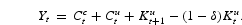
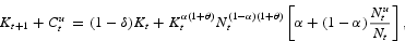
The homogeneous consumption/investment good, Yt, is produced by competitive firms using the following production technology:
where
and
denote for the economy-wide averages of capital and labor in period t; increasing returns are measured by the parameter θ≥0.
Profit maximization leads to the following set of conditions:
Households
We build on Woodford's [1986] work but depart from it by assuming that both types of households supply variable labor. The crucial feature of the model is that the access to credit is imperfect and asymmetric. Specifically, we make the assumption that some households are not able to borrow against their expected wage income. A liquidity constraint is thus imposed on these households: They can not finance their current expenditures out of their cash balances held at the outset of the period or out of their end of period capital income. We do not attempt to derive such a constraint endogenously. However, it might arise as an equilibrium phenomenon in the presence of repayment enforcement or information problems.
Constrained households
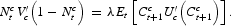
Constrained households value consumption and leisure according to (the superscript c stands for constrained):
where Ctc denotes consumption and
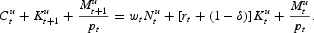
denotes hours worked; λ∈(0, 1) is a discount factor. The momentary utility function satisfies usual properties. Constrained households maximize their expected utility (3) subject to the sequence of constraints:
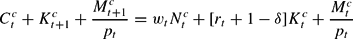

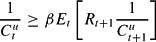
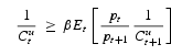
for pt the price level, wt the real wage, rt the rental rate on capital and δ the rate of capital depreciation. Here (4) is the households' wealth constraint, and (5) is the liquidity constraint. The necessary first-order conditions are:

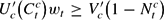
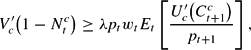
where Rt+1≡rt+1+1−δ denotes the gross rate of return on capital. Relations (6), (7) and (8) hold with equality if
, the liquidity constraint (5) does not bind and
, respectively.
In the sequel, we will focus on equilibria in which
and the liquidity constraint (5), which boils down to a typical cash-in-advance constraint whenever
, is binding (reasons are discussed later). In such circumstances the constrained households' behavior is described by:
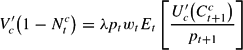


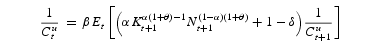
We can use equations (9), (10), and (11) to obtain:
For future reference, let
, for
and
the absolute value of the elasticity of the marginal utility of leisure and consumption, respectively. It is not difficult to see that 1/(ε−1) is the elasticity of the labor supply with respect to the real wage.
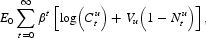
Unconstrained households
The second type of households do not face the same kind of credit limits. This is equivalent to saying that these households are able to borrow against labor income expected to be received during the period. Accordingly, they maximize (the superscript u stands for unconstrained):6
We adopt the logarithmic specification for simplicity.
subject to the sequence of wealth constraints:
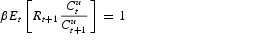
The necessary first-order conditions are:
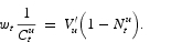
Relations (15) and (16) hold with equality if
and
, respectively. We shall focus on equilibria in which (see the discussion later):

so that the money is dominated by capital in returns. This entails that unconstrained households are unwilling to hold cash balances, that is,
. Their behavior is thus described by:


For future reference, let
denote the unconstrained households' Frischian elasticity of labor supply.
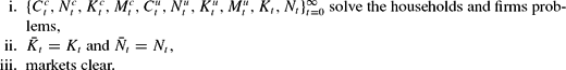
Equilibrium
A symmetric equilibrium consists in a set of prices
and external effects
such that, given these prices and externalities:
As mentioned earlier, the equilibria we shall focus on are such that constrained households choose not to hold capital (
) and are forced to hold money by the cash-in-advance constraint, whereas unconstrained households own the whole stock of capital and hold no money (
). This assymetry stems from the heterogeneity in time preferences, that is, discount rates. To see this, first notice that along a deterministic steady state conditions (6) and (15) imply 1≥λR and 1≥βR, respectively. In equilibrium, it must be the case that some households hold productive capital, hence at least one of the previous inequalities must hold with equality. Naturally, whenever constrained individuals discount the future more heavily than unconstrained ones, that is, λ<β, the only possibility consistent with an equilibrium where both assets are held is 1>λR and 1=βR. This clearly entails a concentrated ownership of capital: Ku>0 and Kc=0.7
As a matter of fact, at the “low” ongoing rate of return on capital, impatient constrained households would rather borrow, if they could, rather than save.
To sum up, heterogeneity in individuals' discount rates (λ<β) and constant money supply (Mt=M) guarantee that along the steady state unconstrained households hold capital and no money, whereas constrained households hold no capital and are forced to hold money by their (binding) liquidity constraint. By continuity, these results will continue to hold in a sufficiently small neighborhood of a steady state. Therefore, in the vicinity of a steady state the optimal choices of constrained and unconstrained households are well described by the conditions (12) and (19)–(21), respectively.
We now give the equations governing the equilibrium dynamics in the vicinity of the steady state, which is unique under our assumptions. An equilibrium is a set
satisfying (1)–(2), (12), and (19)–(21). Because
, the market clearing conditions are particularly simple:


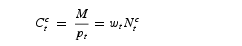
The money market clearing condition (24) deserves some comment. Recall that the money supply is constant. As money is only held by constrained households, equilibrium in the money market means that real balances M/pt is equal to their consumption Ctc and to their wage income
. It follows, and this will turn out to be essential in the sequel, that constrained households consume their wage income immediately, that is,
.
It is now straightforward to see that nearby the steady state, there exists a nonstationary equilibrium sequence
satisfying:

where

LOCAL DYNAMICS
This section characterizes the local dynamics of the economy around the steady state. For that purpose, let
, where the hats indicate percentage deviations from the steady state. The log-linear approximation of the equilibrium system (26)–(29) is of the form:
where M1 and M2 are 3×3 matrices. Now, introduce the vector of Euler equation errors:

that satisfies Et[Φt+1]=0.8
The capital being a predetermined variable, the last component of Φt+1 is nil as Et[Kt+1]=Kt+1.
The matrix M1 is assumed to be nonsingular.
where
and
.
The properties of the set of stationary solutions of equation (32) heavily depend on the value of the eigenvalues of the Jacobian matrix J or, more specifically, on the dimension of the stable subspace of J. For instance, stable solutions exist if one can choose expectation errors, that is, the components of et+1, so as to eliminate the explosive components of Xt.
When the equilibrium is determinate, that is, when J has two eigenvalues located outside the unit circle, one can find two linear restrictions on both Xt and et+1.10
Let J=QΛQ−1 where Λ is a diagonal matrix with the eigenvalues of J on the diagonal and Q is the matrix of eigenvectors of J. The linear restrictions afore-mentioned are found by setting the rows of Q−1Xt and Q−1et+1 associated with the two explosive eigenvalues of J equal to zero.
and
, as linear functions of the predetermined variable,
. Those on et+1 imply that the expectation errors, et+1 and
, are equal to zero in every period. Therefore, extrinsic beliefs do not matter.
When instead the equilibrium is indeterminate, that is, when J has one or zero eigenvalue lying outside the unit circle, there is no longer enough restrictions on Xt in order to pin down the nonpredetermined variables. Accordingly, the state space now includes
or/and
, depending on the number of unstable eigenvalue. Moreover,
and
can be different from zero as long as
, i=1, 2. In such a case, the forecast errors can be written:
, where the zero-mean random variable κ stands for the sunspot.11
When, as it turns out to be the case in this model, the steady state is a saddle with one dimension of instability, the expectation errors are not linearly independent. We have
, which may rewrites as
with η2=νη1.
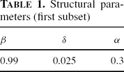
The model exhibits indeterminacy whenever J has at least two eigenvalues of modulus less than one. Because the analytical characterization of the eigenvalues of the 3×3 matrix J is cumbersome, a numerical procedure will be considered. Following the existing literature, we calibrate our model by setting the time interval to be a quarter; Table 1 summarizes the calibration for a first subset of parameters.
Recall that in Woodford's [1986] formulation owners of capital, that is, unconstrained households, do not work. In order to meaningfully highlight the role played by the supply of labor of capital owners, we first reassess the case studied by Barinci and Chéron (2001), where the labor supply of constrained households is infinitely elastic, that is, ε=1. We calculate the minimal value of θ giving rise to indeterminacy, for various values of the unconstrained households' elasticity of labor supply, εu, and share in total hours,
. Table 2 reports some results. Case 1 (inelastic unconstrained households' labor supply) is a lot like the one in Barinci and Chéron (2001), where capital owners do not work. It turns out that with this parameterization, our economy displays indeterminacy when θ>0.28.12
This minimum returns to scale differs slightly from the one in Barinci and Chéron (2001) because they consider increasing returns exclusively driven by labor externalities.
In order to get some intuition about the occurrence of indeterminacy, consider the effects of an optimistic shock to the beliefs. Constrained households expecting higher rate of return on money, that is, waiting for more consumption tomorrow, increase their hours worked. Unconstrained households then expect a fall in the real wage, together with an increase in the rate of return on capital. These expected prices dynamics cause them to supply more labor and to invest more instantaneously. This allows for more output and consumption tomorrow, eventually validating the beliefs of households. The elasticity of the unconstrained households' labor supply plays a key role. The fact that optimistic beliefs of constrained households cause unconstrained ones to supply more labor enhances the impact of the initial shift of labor on the rate of return on capital and investment. This complementarity between the constrained and unconstrained households labor supply, in making more likely the rise of future output and consumption consistent with initial beliefs, acts in place of large increasing returns. The weight of unconstrained workers in total hours plays a role, too. The higher this weight, the more marked the rise of investment, hence, future output and consumption, following a sunspot shock. This makes more likely the occurrence of indeterminacy.

The previous results have been obtained for ε=1. To what extent do they rely on this assumption? In other words, how sensitive is the critical level of increasing returns with respect to the constrained households' labor supply? To shed some light on this issue, consider the iso-elastic utility functions
and
. Then
. One sees that ε=1 requires both risk-neutrality (σ=0) and infinite Frischian labor supply elasticity (η=0).13
The linearity in leisure can be justified by appealing to the arguments for indivisible labor in Hansen (1985).
We set εu=1 and
.

BUSINESS CYCLE PROPERTIES
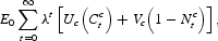
This section presents a quantitative evaluation of the model, thereby providing an appraisal of the mechanism through which variations in beliefs are propagated over time. For comparison purposes, we contrast the predictions of our model (hereafter BCL) with those of two benchmark models: the standard RBC model driven by permanent technology shocks, and the two-sector EBC model driven purely by sunspots analyzed by Schmitt-Grohé (2000) (hereafter SG).
Simple Measures of Comovements
Following a common practice, the empirical performance of our business cycle model is judged by its ability to match unconditional second moments of key macroeconomic aggregates. The model moments are computed from the stochastic system equation (32) making use of the baseline calibration in Tables 1 and 4.15
Jappelli (1990) and Diaz-Giménez, Quadrini, and Rios-Rull (1997) have provided evidences that around 25% of U.S. households are virtually liquidity constrained. Accordingly, we fix the constrained households share of labor at
.
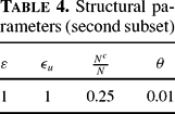
Table 5 reports the predicted second moments for growth rates and their empirical counterparts. The first panel presents the standard deviation of per capita consumption growth relative to the standard deviation of the output growth, and the cross-correlation between these two variables. The second and third panels report the same statistics for per capita investment growth and detrended per capita hours. The first columns of these three panels report the estimates based on U.S. quarterly data covering the period 1948:Q3-1997:Q4; asymptotic standard errors are in parentheses.

Table 5 illustrates the ability of the RBC model to fit the relative volatilities of consumption and investment growth with respect to output growth. However, the model predicts hours growth that is too smooth relative to output growth. Both EBC models generate relative volatilities of investment and hours growth significantly larger than in U.S. data. The relative volatility of consumption is the only fact matched by the three models.
As regards to contemporaneous correlations between output growth and consumption, investment and hours growth, respectively, the RBC model predicts statistics close to one, whereas in data such high correlations are always rejected. Nonetheless, it is fair to notice that the sign of these correlations is correctly predicted. On the contrary, and this is probably its main shortcoming, the SG model produces a time series for consumption that is countercyclical.16
Moreover the volatility of hours and investment relative to the output growth is excessive.
If the wage instead rises, for instance because of the presence of large increasing returns as in Benhabib and Farmer (1994), which entails upward-sloped labor demand schedule, consumption could be procyclical.
Even though the BCL model has some weaknesses, notably regarding the relative standard deviations of hours and investment, it not does not face the well-documented consumption “anomaly” of sunspot fluctuations models: It successfully predicts the positive instantaneous correlation between output and consumption. Moreover, it succeeds in replicating the lead-lag pattern of consumption over the cycle, whereas both SG and RBC models fail to account for this fact. The mechanism behind the procyclicality result is simple. As in equilibrium the liquidity constraint is binding, the constrained households' intratemporal marginal efficiency condition does not hold with equality. Accordingly, consumption and hours worked are not forced to move in opposite directions. In fact, constrained households consume their current labor income [see equation (24)], and this “Keynesian-like” behavior in terms of consumption explains the relevancy of the propagation of sunspot shocks in the BCL model economy.
Forecastable Comovements in Main Aggregates
Any useful model of the business cycle should provide accurate forecasts of main macroeconomic aggregates. However, Rotemberg and Woodford (1996) argue that the standard RBC model generates counterfactual comovements between the forecastable component of output, consumption, investment, and hours fluctuations. Estimating a VAR model between U.S. output, consumption, investment, and hours, they are able to recover the expected movements of the aggregate variables. They then compute the correlation between these components at several leads and lags. Table 6—lines 1 to 3—reports the estimated values obtained by Rotemberg and Woodford (1996). It shows that predictive changes in output are strongly correlated with the predictive changes in consumption, investment and hours.18
A comparison with the unconditional moments reported in Table 5 indicates that the correlation between forecasts is larger than between the overall changes, notably for consumption.
Rotembreg and Woodford (1996) perform the same exercise on simulated series obtained from the standard RBC model, and establish that this model can not replicate the data. Schmitt-Grohé (2000) recently reaches the same conclusions regarding the two-sector EBC model (see Table 6). These counterfactual results can be explained as follows.

RBC
Following a positive and permanent technological shock, the inherited capital stock is below its steady state value. Then, its marginal product is above the steady state. Under standard parameterizations, this leads households to enjoy less consumption and leisure than in the steady state. Consequently, consumption is expected to rise, whereas hours worked are expected to decline. Provided that the labor share is sufficiently large (it is set at 0.7 in our calibration) the initial level of hours implies that output approaches its steady state value from above. Overall, the RBC model predicts that when output and hours fall, consumption rises.
SG
Following a sunspot shock, labor supply increases. As long as the labor-demand schedule slopes downward, the wage falls. If consumption and leisure are normal goods, the intratemporal efficiency condition forces consumption to decrease. Consequently, in the transition toward the steady state consumption is forecasted to increase, whereas output is expected to decline.19
It is worthy to note that the allowance of permanent technological shocks is not sufficient to overcome this shortcoming, whereas it allows the model to capture the positive unconditional correlation between consumption and output [see Schmitt-Grohé (2000)].
Table 6 illustrates that, in sharp contrast to RBC and SG models, the BCL model implies positively correlated forecastable changes in consumption and output. The economic mechanism that creates this result can be understood as follows. If financially constrained households expect an increase of the real return on money, they wait for more consumption tomorrow and thus supply more labor today. Unconstrained households then anticipate higher return on capital. Under usual utility specifications, they supply more labor and raise their investment. The increase of labor supplies entails a large rise of the current return on capital, hence of investment, allowing for more output and consumption in the current period. Thereby, along the transition path output and consumption are expected to decrease.
CONCLUSION
This paper has established that imperfect financial markets significantly improve the propagation of sunspot impulses. We have proposed a one-sector model with heterogeneous households and liquidity constraints, which is able to overcome some of the criticisms that have been addressed to both standard RBC and EBC models. The most noteworthy improvement is that the model exclusively driven by sunspot shocks can account for the joint dynamics of output and consumption. More specifically, it does a pretty good job in matching the unconditional and predictable movements in output, hours, and consumption, which are defining features of the business cycle fluctuations that available EBC models have not been able to capture.
We wish to thank an anonymous referee, an associate editor, and Fabrice Collard for very helpful comments. We also thank Stéphanie Schmitt-Grohé for providing us her data bank.


